Decoherence induced by Smith-Purcell radiation
Abstract
The interaction between charged particles and the vacuum fluctuations of the electromagnetic field induces decoherence, and therefore affects the contrast of fringes in an interference experiment. In this article we show that if a double slit experiment is performed near a conducting grating, the fringe visibility is reduced. We find that the reduction of contrast is proportional to the number of grooves in the conducting surface, and that for realistic values of the parameters it could be large enough to be observed. The effect can be computed and understood in terms of the Smith-Purcell radiation produced by the surface currents induced in the conductor.
pacs
PACS number(s):03.65.Yz,03.75.DgI Introduction
The interaction of a quantum system with its environment produces decoherence, which is one of the main ingredients to understand the quantum to classical transition zurek. If an interference experiment is performed with charged particles, the unavoidable interaction with the vacuum fluctuations of the electromagnetic field induces decoherence, and therefore affects the visibility of the fringes bp-mpv. Indeed, in previous papers it has been shown that the presence of a perfectly conducting plane surface has a small influence on the contrast of the fringes. This was originally pointed out in Ref. ford, and the results were subsequently revised and generalized in Ref.mpv. The interaction with the vacuum fluctuations of the electromagnetic field can enhance or suppress the contrast with respect to the visibility in vacuum (absence of conducting plane), depending on the relative orientation of the conducting plane and the plane of the trajectories of the particles mpv. The modification of the visibility of the fringes can be understood in very simple terms imry: if an electron moves with a typical frequency along the trajectory of the experiment, and if the two trajectories are separated by a distance , the fringes visibility decays a factor , where is the probability that a dipole oscillating at a frequency emits a photon. If the experiment is performed in front of a conducting plane, the image charges enhance the effect when the conductor is perpendicular to the plane of the experiment. Alternatively, the image charges suppress the decoherence when the trajectories are contained in a plane parallel to the conductor. In principle, a similar effect is present for neutral particles with electric and/or magnetic dipole moment mpv.
As is proportional to , where is the mean velocity of the particles with charge , this effect is extremely small, and therefore very difficult to observe, unless the charged particles are made to oscillate many times before reaching the screen mpv. There are variants of the above mentioned configurations in which the decoherence is notably larger. For example, it has been argued that if a double slit experiment is performed over a non-perfect conductor, the image charges in the material will dissipate energy through Joule heating, and will also affect the visibility of the fringes anglin. This effect has been further analyzed in Refs. mach; levinson, where the interaction of the interfering wave packets with the electrons in the macroscopic body has been modelled using different approaches. A recent experiment has confirmed that the presence of a semiconducting plate induces decoherence sonnen, although the agreement between theory and experiment is still not perfect. Another possibility to control the decoherence in a double slit-like experiment is to perform it in the presence of a classical electromagnetic field ford2; lmv. When this is sufficiently intense, random phases coming from the emission time of the wave packets can also induce a large amount of decoherence.
In this paper we will explore another configuration that will also prove to be potentially interesting from an experimental point of view. When a charged particle moves with constant velocity over a perfectly conducting grating, the currents induced in the surface of the conductor produce radiation, that can be intuitively understood as coming from the oscillating image charge. This is the so called Smith-Purcell effect spe. We argue that, because of this radiation, if a double slit-like experiment is performed near a conducting grating, there will be a suppression of the interference fringes. Moreover, we expect the effect to be enhanced by the number of grooves in the conductor, and therefore it is more likely to be observed than previous proposals in Ref. ford; mpv.
The paper is organized as follows. In the next Section we present the main formalism and a formula which, in principle, gives the decoherence factor for a double slit experiment performed near a conducting surface of arbitrary shape. We follow closely Ref.mpv. In Section 3 we evaluate the decoherence factor for the particular case of a conductor with a periodic grating. We argue that, under reasonable assumptions, the reduction in the visibility of the fringes can be estimated using a quasi equivalent system formed by the original charges and their images in vacuum. We show that the decoherence factor is proportional to the number of grooves. In Section 4 we discuss the experimental feasibility of our proposal and include our main conclusions. Some details of the calculations are relegated to the Appendix. Along this work we use natural units, .
II Fringe visibility in a double slit experiment with boundary conditions
Let us consider a double slit experiment performed with charged particles (electrons). Assume that the two electron wave packets follow well defined trajectories and that coincide at initial () and final () times. In the absence of environment, the interference depends on the relative phase between both wave packets at . Because of the interaction with the quantum electromagnetic field, the interference pattern is affected. We assume an initial state of the combined particle–field system of the form . Here is the initial (vacuum) state of the field and are two states of the electron that are localized around the initial point and that in the absence of other interaction continue to be localized along the trajectories respectively. At later times, due to the particle field interaction the state of the combined system becomes
| (1) |
Thus, the two localized states and become correlated with two different states of the field. Therefore, the probability of finding a particle at a given position turns out to be
| (2) | |||||
The absolute value of the overlap factor is responsible for the decay in the fringe contrast, which is the phenomenon we will analyze here. Calculating it is conceptually simple since is nothing but the overlap between two states of the field that arise from the vacuum under the influence of two different sources (this factor is identical to the Feynman–Vernon influence functional Feynman-Vernon). Each of the two states of the field can be written as
| (3) |
where is the conserved –current generated by the particle following the classical trajectory , i.e. , (). Using this, the simplest way to derive an expression for the overlap is based on the observation that as the QED action is quadratic in the fields, the overlap must be a Gaussian functional of the two currents and . Thus, we can write the most general Gaussian functional ansatz for as
| (4) | |||||
where a summation over the indices is implicit. On the other hand, we can explicitly write down the expression for the overlap as
| (5) | |||||
The kernels and appearing in (4) can be determined by identifying the functional derivatives of equations (4) and (5). In this way, one can relate and with the one and two point functions of the field operators. As we are only interested in the absolute value of the overlap, we will only present the result for this quantity here. Denoting , we get
| (6) |
where is the expectation value of the anti–commutator of two field operators:
From the above derivation, it is clear that the the square of the overlap has a simple physical interpretation: is equal to the probability for vacuum persistence in the presence of a source , which corresponds to a time dependent electric dipole imry. This is of course not a physical dipole but a fictitious one, formed by the difference of the currents associated to the wave packets that follow each interfering trajectory. The information about the existence of a conducting shell is encoded in the two-point function of the electromagnetic field.
The overlap factor has been computed in Ref.mpv, both in vacuum and in the presence of a conducting plane, by considering the appropriate two-point functions. If we denote by the result in empty space and by the result in the presence of a conductor, the overlap factor is given by when the trajectories are parallel to the conductor (recoherence) and by when the trajectories are perpendicular to the conducting surface (decoherence). These results, valid when all trajectories are very close to the conductor, can be reproduced using the method of images and taking into account that decoherence in empty space is related to the probability of photon emission for the fictitious varying dipole . When the conducting plane is parallel to the dipole, the image dipole is . Therefore the total dipole moment vanishes, and so does the probability to emit a photon in the leading order approximation. The image dipole cancels the effect of the real dipole and this produces the recovery of the fringe contrast with respect to the empty space case. On the other hand, when the conductor is perpendicular to the trajectories, the image dipole is equal to the real dipole . Therefore, the total dipole is twice the original one. This in principle would lead us to conclude that the total decoherence factor should be four times larger than . However, in the presence of a perfect mirror photons can only be emitted in the region. This introduces an additional factor of that gives rise to the final result. The conclusion is that one can replace the original problem by an equivalent one in which the conducting plane is replaced by the image charges. The overlap factor can be computed using the two-point function of the electromagnetic field in empty space, by including the appropriate image charges. In the next Section, with the aim of seeking an enhanced observable which could be measured in present experiments, we will use this equivalence to compute the overlap factor in a more complex geometry.
III Induced decoherence in trajectories above a grating conductor
We will now analyze an interference experiment in which a charged particle moves above a conducting medium with periodic grating along two possible different paths. We expect that, within the proper approximations, the radiation emitted by the accelerated image charges leave imprinted the which-path information in the electromagnetic field, inducing in this way decoherence and, therefore, a loss of contrast in the interference fringes.
We consider an experimental setup in which an electron moves in two possible trajectories above a conducting plate with a periodic grating. The grating shape below each trajectory has no need of being equal to each other. In particular, we study here the two trajectories in Figure 1a, where the electron travels at a height above the conductor’s surface, and the conductor’s surface consists in a grating of spatial period and groove’s depth . In order to calculate the overlap factor, one should be able to compute the two-point function of the electromagnetic field appearing in Eq. 6, in the presence of the grating. Alternatively, one could model the currents induced in the conducting surface and use the empty space two-point function. Indeed, this approach has been considered in the literature in order to calculate the radiated intensity distribution produced by an electron beam passing over a metallic grating Brownell98. A third possibility, when the geometry of the conductor allows it, is to use the method of images to reproduce the effects of the surface currents.
In this article, without loosing the sought effect and for the sake of simplicity, we analyze the problem as if an electron’s image charge is placed below the conducting plate surface and performs a trajectory with non-uniform vertical velocity which depends on the grating shape, as shown in Figure 1b. This could be achieved, for instance, if the grating behaves as a periodic array of horizontal ”infinite planes” connected by sloping surfaces, giving the usual image charge everywhere but on the position of the slopes, where we model the surface current as an image charge with non vanishing vertical velocity, going from one plane to the next one. To validate this simplified model we will assume . We may refer to this as a proximity approximation. Moreover, to avoid the problem of non physical velocities for the image charges, we will assume that the slopes are not very steep. The method of images has already been considered to compute the intensity distribution of the Smith-Purcell radiation Ishiguro, as well as to model the induced retarded currents in the conductor Brownell98.
We argue that, within this proximity approximation, the decoherence factor corresponding to the experimental setup of the charge moving in two possible paths above the conducting surface equals one half of the decoherence factor produced by two charges (one equal to the real charge and other equal to its image) in vacuum which travel in two possible paths each one of them. The factor comes from the double counting of radiation in the quasi-equivalent setup. The two currents which interfere in this scheme are
| (7) | |||||
| (8) |
with
| (9) |
The superscripts and stand for above and below, respectively (the above currents correspond to the physical charges, while the below currents describe the image charges), is the electron’s trajectory in the -direction, is the trajectory in the -direction for the image charge, and depending on the relative shape of the gratings in the conductor below each trajectory in the original setup. means that below one of the trajectories there is a grating and below the other the conductor is flat; means that the perturbations in the conductor’s surface (relative to a flat surface) in each path are exactly the same; and means that the perturbations in each path are opposite, i.e., if at a given point in one of the paths there is a valley in the perturbations, then at the equivalent point in the other path there is a peak. These particular values for will allow us to explore the effect of different gratings below each path of the original setup.
Defining
| (10) |
with , it is straightforward to obtain the decoherence factor for the original setup that, in virtue of the emitted Smith-Purcell radiation, will be denoted by :
| (11) |
where is the contribution that corresponds to the interaction between the above currents, to the interaction of the above currents with the below currents, and so on. The two-point function of the electromagnetic field is the free two-point function, that in the Coulomb gauge reads
| (12) |
where . By computing explicitly the different terms in Eq. 11 it is easy to obtain that, for instance, (the result for empty space produced by the currents above the conductor). Moreover, if we define
| (13) |
with no sum on and , in such a way that , it is easy to see that
| (14) |
That is, if we do not include the -component of the currents in the computation of , we retrieve the decoherence factor for a plane conductor. Therefore, the decoherence factor due to the grating in the conductor equals the factor associated to a plane conductor plus a modification,
| (15) |
where comes from the terms containing a non-vanishing -component of the velocity,
| (16) |
Suppose now that the grating in the conductor has grooves, such that the vertical velocity of the image charges can be modelled as
| (17) |
where corresponds to the velocity shape each time there is a steep in the conducting surface, is the time it takes the charge to go from one steep to the next, , and the factor accounts for the upwards and downwards steeps. (Observe that is different from zero only in , where is the time it takes the charge to go over the steep.) Once we have modelled as the sum in Eq. 17, we realize that the different terms in the RHS in Eq. 16 will contain either one of these sums ( and ) or a modulus square of this sum (), depending on how many times the -component of the below currents is present in them. For example
| (18) | |||||
The modulus square in gives rise to terms in which the phases in the sum in Eq. 18 are exactly cancelled and, hence, they are relatively enhanced in comparison to the contribution coming from the remaining terms. Indeed, these other terms with correspond to the interaction of the currents in the -th and -th steeps, and we expect them to vanish for (or equivalently ) large enough. In fact, this is the case, since for the phase factor’s frequency as a function of is at least , whereas the ’s Fourier transform has a typical width of , therefore the -integration gives a strong suppression if this Fourier transform is well behaved. If then the contribution of these terms also depends on the relationship between and , since for we may have that the current coming from the -th steep in one path interacts with the current coming from the -th steep in the other path. The detailed analysis of this discussion is relegated to the Appendix, where we show that under the reasonable conditions (and for ), the following approximation hold,
| (19) |
Here is the same as but replacing in the expression for the -current, Eq. 9, i.e., it corresponds to the decoherence factor of only half oscillation in the -direction. Under the same conditions, one can show that
| (20) |
i.e. the leading contribution to the decoherence comes from the term which is quadratic in the vertical component of the velocity (see Appendix).
Integrating and in Eq. 13 it is straightforward to obtain
| (21) |
where we have used and since, for simplicity, we are assuming a non-relativistic regime.
To summarize, we have found that for a double slit-like experiment above a flat conducting plate, if the flat surface is changed to a grating surface with grooves, then the decoherence factor is enhanced as
| (22) |
This is the main result of this article. Notice that this effect is due to the acceleration of the image charge at the sloping surfaces, hence the effect is proportional to and, as far as , is independent of .
An estimation of the enhancement in Eq. 22 needs a calculation of . The precise value of , however, needs the function , the distance between both paths, , and a value for . Nevertheless, we may study its generalities and then examine a particular example with a given function .
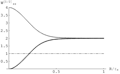
As a first observation notice that, in the case , the decoherence factor is independent of . This is to be expected, since the Smith-Purcell radiation is in this case entirely due to the image charge that corresponds to the trajectory that lies on the grating. For , the magnitude in Eq. 21 should be compared to the wavelength of the typical most energetic photons emitted by an electron in a trajectory . Therefore, unless abruptly accelerated trajectories, should be compared with . For instance, if we take then for values of where ’s Fourier transform is not negligible. Hence, in the case of coincident trajectories (), we find a suppression in the decoherence factor through in Eq. 21. In fact, this is expectable from first principles: if the electron oscillate in concordance in both paths and the photons wavelength is greater than the distance between both paths, then we cannot expect to be able to obtain the which-path knowledge from the information imprinted into the electromagnetic field. On the other hand, if the electron has opposite oscillations in each path –this is achieved by using –, then we should expect to have decoherence independently of any cutoff in the spectrum of the photons emitted by the accelerated image charges. This is in fact the case, since and imply and a value for four times larger than the case , hence there is not suppression for in this condition.
In the other limit case, , we expect the photons to carry the which-path information and to produce decoherence independently of concordant () or opposite ( trajectories of the image charges in the -direction. In fact, writing the factor in the integral in Eq. 21
| (23) |
we see that in both cases this factor is a constant contribution plus or minus rapid -oscillating contributions. Since these oscillating factors are integrated with the modulus square of the Fourier transform of , we find that the oscillation cancels the integral for . Therefore, we have that when the distance between both paths is large enough, the decoherence factor is independent of the value of and equals twice its value when :
| (24) |
As an example we study here the behavior of for a particular value of , which corresponds to a given shape in the conductor’s surface. We first study analytically the behaviour of for this in the case , and then we study numerically its behaviour for and arbitrary values of .
We take a which has two periods of constant acceleration in such a way that its -integral equals , the groove’s depth. Defining as the typical velocity of the system, we have
| (25) |
which, through Eq. 21 and Eq. 22, yields
| (26) |
where is the mean angle of the sloping surfaces. As expected, the decoherence increases as the slopes become more abrupt. Although this conclusion is achieved within a non-relativistic image-method approximation, it is expected to be valid beyond it: an extremely abrupt slope will induce surface currents with a greater time dependence, which will generate decoherence through its radiation.
As it can be seen from this result, Eq. 26, the decoherence factor is suppressed by a factor. (This is an expected suppression and it was already noticed in Ref.mpv.) However, the complete decoherence factor is enhanced by an factor due to the grooves in the conductor’s surface. This enhancing factor coming from the Smith-Purcell emitted radiation may counterbalance the suppression and hence provide visible effects of decoherence due to a modification of the electromagnetic boundary conditions in a typical interference experiment.
The study of in the cases for arbitrary values of is easily managed numerically, once the general analysis has been performed. In Fig. 2 we plot the decoherence factor corresponding to the velocity given in Eq. 25 for as a function of . As expected from the above discussion, converges to when (see Eq. 24).
As it can be seen, the above results are independent of and . This is expected in our image-method approximation, which is valid if . Observe that, in order to validate the approximations, the constraint is also needed in the cases or , although does not appear in the result for (Eq. 26 and Fig. 2).
IV Discussion and experimental perspectives
In this article we have proposed a concrete setup to carry into effect the idealized experiment discussed in Ref.mpv, in which the electron in a double slit experiment above a conducting plane oscillates times before reaching the screen in order to increase the decoherence factor. In the present simple setup, a double-slit experiment for charges is performed above a grated conducting surface. Although the electron wave packets move with constant velocity above the grating, the image charges oscillate many times in the vertical direction due to the presence of the sloping surfaces. These oscillations leave an imprint in the electromagnetic field through the Smith-Purcell radiation, and therefore produce the sought enhancement in the decoherence factor.
We have made several assumptions in order to simplify the estimation of the Smith-Purcell induced overlap factor, which turns out to be , where is a constant of order one that depends on the details of the conducting surface. In particular, we have assumed that the motion of the charged particles and their images is non relativistic. This is a very conservative assumption, and the effect could be larger by considering other gratings with abrupt changes in the surface, or composed by a periodic array of conducting slabs separated by vacuum gaps. Even within our conservative assumptions, the effect could be large enough to be observed. As a concrete example, the evaluation of Eq. 26 for the case of an electron flying above a groove’s grating with and a velocity and slopes such that , yields that the fringe visibility is reduced by a factor . According to our approximations, this may be experimentally achieved by setting , , and of the order of . This yields a total length for the conductor of about cm.
At this level of approximation () the decoherence factor is independent of and . For we should expect the same dependence as in the radiated power of the non-relativistic Smith-Purcell effect, which is dominated by the exponential factor xxx. However, if we go beyond our approximation, we should also expect that the enhancing envisaged in Eq. 26 due to abrupt grooves becomes a computable large factor for gratings with .
At last, notice that an electron flying over a conductor –not necessarily grated– may induce an extra source of decoherence due to dissipation of energy of the image charge in the conductor and this could mask the Smith-Purcell decoherence. This dissipative effect was theoretically modelled by Anglin and Zurek anglin and by Machnikowski mach and recently measured by Sonnentag and Hasselbach sonnen. The measurement of the effect still does not confirm any of the two models. In particular, the dependence of the effect with the resistivity of the material () is quite different in the two theoretical predictions and further experimental analysis –as repeating the experiment in sonnen with different materials– is required in order to clarify this issue. Using the experimental results in sonnen for a semiconductor with m, and the -dependence predicted by Anglin and Zurek, the decoherence due to dissipation for the above proposed experimental parameters using a grating of copper at room temperature ( m) would be negligible. On the other hand, if we assume Machnikowski’s model, the dissipative decoherence could be comparable or greater than . However, both models agree that if the temperature is lowered by at least two orders of magnitude then could be observed, independently of possible dissipative effects.
The estimation of the overlap factor can be improved in several directions, since we have used a crude approximation to model the surface currents on the grating. A more rigorous approach, based on Eq. 6 with a complete evaluation of the two-point function in the presence of the grating, could show important deviations from our proximity approximation, in particular for non-smooth surfaces, producing an enhancement of the effect.
Acknowledgements.
We thank F. Lombardo for carefully reading this manuscript. We also thank D. Dalvit for comments about the validity of the ”proximity” approximation in this context. This work has been supported by Universidad de Buenos Aires, CONICET and ANPCyT.Appendix A
In this Appendix we prove the validity of Eqs. 19 and 20. To demonstrate Eq. 19 we integrate and in the expression for , Eq. 13, and replace the velocity by its expression in Eq. 17. After performing the change of variables in both -integrals and using , we obtain
| (27) | |||||
It is clear that there are equal terms in the summation for which and, hence, give rise to a contribution. Now we should show that the contribution coming from the –terms is negligible in comparison to . Although this might look straightforward since these other terms have an -oscillatory phase which should suppress their contribution due to the -integration, one must be aware that there are of these –terms.
For the sake of simplicity we present the detailed proof for the case , the other possible cases are analyzed below. The relevant integral in Eq. 27 in this case is
| (28) |
where the change of variables has been performed and has been used where possible. Since the argument of the exponential cannot be zero we can perform the -integration in the distributional sense and get
| (29) | |||||
| (30) |
where in the last step we have assumed in the denominator, and we have integrated and to obtain the height of the steep, . At this point we see that the terms are combined in a sum which can be exactly computed for large to give at leading order,
| (31) |
Having into account that in general , we conclude that implies and, therefore, we can approximate
| (32) |
as we wanted to show.
The case is now easily worked out. In this case we need to analyze a similar as above, but now with a factor within the integral. This extra-factor ends up giving a correction to the argument of the exponential in Eq. 28 which now reads , where
| (33) |
is an angular factor associated to the -integration such that . Therefore, if we assume –to avoid the possibility that the argument of the exponential vanishes–, then we can proceed in a similar way as before and reach the same conclusion. Notice that for close to its larger limit, when takes values close to the approximation that goes from Eq. 29 to Eq. 30 could be spoiled for the very first terms where , but this does not modify our general conclusion.
Let us now consider the inequality in Eq. 20, . Once has been analyzed, we can easily study the qualitative behavior of , , and . We analyze in detail , but the same arguments are valid as well for the others.
Once we compute using Eq. 13 and Eq. 17, we see that its expression contains only one sum, instead of two. Therefore, at difference of the case, there is no cancellation of the phases that arise from the change of variables within one of the integrals. We have that the relevant part of the integral in looks like
| (34) |
Assuming that both Fourier transform within the -integral are well behaved, we see from here that almost all terms in the sum will have an oscillatory factor which will suppress the contribution of the -integral. Moreover, the expected peak around from the first Fourier transform will be suppressed by the factor in the integral. Therefore, we can expect the contribution of to be negligible in comparison to which is enhanced by . The same arguments apply as well for , and .
References
- (1) For a review see J. P. Paz and W. H. Zurek, in ”Coherent matter waves, Les Houches Session LXXII”, edited by R Kaiser, C Westbrook and F David, EDP Sciences, Springer Verlag (Berlin) (2001) 533-614.
- (2) H.P. Breuer and F. Petruccione Phys. Rev. A63, 032102 (2001); P.M.V.B. Barone and A.O. Caldeira, Phys. Rev. A43, 57 (1991).
- (3) L. Ford, Phys. Rev. D47, 5571 (1993); L. Ford, available at hep-th/9408172; L. Ford, Phys. Rev. A56, 1812 (1997).
- (4) F.D. Mazzitelli, J.P. Paz and A. Villanueva, Phys. Rev. A68, 062106 (2003).
- (5) A. Stern, Y. Aharonov and Y. Imry, published in “Quantum coherence”, edited by J. Anandan, World Scientific (1991); A. Stern, Y. Aharonov and Y. Imry, Phys. Rev. A41, 3436 (1990).
- (6) J. R. Anglin and W. H. Zurek, in Dark Matter in CosmologyQuantum MeasurementsExperimental Gravitation, edited by R. Ansari, Y. Giraud-He´raud, and J. Tran Thanh Van (Editions Frontieres, Gif-sur-Yvette, 1996), pp. 263270; J.R. Anglin, J. P. Paz and W. H. Zurek, Phys. Rev. A55, 4041 (1997).
- (7) P. Machnikowski, Phys. Rev. B73, 155109 (2006).
- (8) Y. Levinson, J. Phys. A: Math. Gen. 37, 3003 (2004).
- (9) P. Sonnentag and F. Hasselbach, Phys. Rev. Lett.98, 200402 (2007).
- (10) Jen-Tsung Hsiang and L. H. Ford, Phys. Rev. Lett. 92, 250402 (2004).
- (11) F.C. Lombardo, F.D. Mazzitelli and P.I. Villar, Phys. Rev. A72, 042111 (2005).
- (12) S.J. Smith and E.M. Purcell, Phys. Rev. 92, 1069 (1953); D.V. Karlovets and A. P. Potylitsyn, Phys. Rev. Special Topics - Accelerator and Beams 9, 080701 (2006).
- (13) R.P. Feynman and F.L. Vernon, Ann. Phys. 24, 118 (1963).
- (14) J.H. Brownell, J. Walsh and G. Doucas, Phys. Rev. A57, 1075 (1998).
- (15) K. Ishiguro and T. Tako, Opt. Acta 8, 25 (1961); W.W. Salisbury, J. Opt. Soc. Am. 52, 1315 (1962). For a more rigorous approach see P.M. van den Berg, J. Opt. Soc. Am. 63, 689 (1973).
- (16) G. Toraldo di Francia, Nuovo Cimento 16, 61 (1960). See also Y. Shibata et al, Phys. Rev. E57, 1061 (1998).