High-Redshift Voids in the Excursion Set Formalism
Abstract
Voids are a dominant feature of the low-redshift galaxy distribution. Several recent surveys have found evidence for the existence of large-scale structure at high redshifts as well. We present analytic estimates of galaxy void sizes at redshifts using the excursion set formalism. We find that recent narrow-band surveys at should find voids with characteristic scales of roughly comoving and maximum diameters approaching . This is consistent with existing surveys, but a precise comparison is difficult because of the relatively small volumes probed so far. At , we expect characteristic void scales of comoving assuming that all galaxies within dark matter haloes more massive than are observable. We find that these characteristic scales are similar to the sizes of empty regions resulting from purely random fluctuations in the galaxy counts. As a result, true large-scale structure will be difficult to observe at , unless galaxies in haloes with masses are visible. Galaxy surveys must be deep and only the largest voids will provide meaningful information. Our model provides a convenient picture for estimating the “worst-case” effects of cosmic variance on high-redshift galaxy surveys with limited volumes.
Keywords:
cosmology: theory – large-scale structure of the universe1 INTRODUCTION
The complex network of filaments and voids observed in the present-day Universe is believed to have formed from an initially homogeneous distribution of matter. In hierarchical models of structure formation, tiny perturbations seeded by the inflationary epoch grew through gravitational instability, collapsing first on smaller scales to form haloes. The subsequent merging and clustering of smaller haloes resulted in the formation of highly structured large-scale systems. Perhaps the most striking characteristic of the Universe today is the prevalence of large and nearly spherical voids in the galaxy distribution. The scales of these voids can be enormous. Indeed, Hoyle & Vogeley 2004 report characteristic radii of with maximum scales approaching in the 2dF Galaxy Redshift Survey.
The characteristics of voids and the galaxies that populate them have been the subject of numerous theoretical and observational studies throughout the years (Gregory & Thompson 1978; Kirshner et al. 1981; de Lapparent et al. 1986; Vogeley et al. 1994; Hoyle & Vogeley 2004; Conroy et al. 2005). To date, these studies have mostly focused on low redshifts. However, it is clear that voids should appear at higher redshifts also. The DEEP2 survey indicates that voids exist at redshifts of (Conroy et al. 2005). Surprisingly, a handful of recent Lyman emitter (LAE) surveys have found hints of large-scale structure at redshifts around (Shimasaku et al. 2003; Shimasaku et al. 2006; Hu et al. 2004; Ouchi et al. 2005).
The modelling of voids poses an interesting theoretical problem. There have been numerous studies utilising -body simulations (Mathis & White 2002; Benson et al. 2003; Gottlöber et al. 2003; Colberg et al. 2005). While these simulations are invaluable tools for understanding the details of void dynamics, they are computationally expensive due to the large volumes and high dynamic range required to include a representative sample of voids while also resolving the much smaller galaxies that define them.
Analytic methods provide a useful alternative. Perhaps the most promising analytic model of void abundances is the excursion set approach taken by Sheth & van de Weygaert 2004. They argue that voids actually provide deeper insight into large-scale structure than halo formation itself. Their assertion is based on the fact that underdense regions generally tend to evolve toward a spherical geometry, making the idealisation of spherical expansion more reasonable. In contrast, gravitationally bound objects typically have geometries that are far from spherical. Approximating gravitational collapse with the spherical model may be highly inaccurate, which partially explains the discrepancies between the Press & Schechter 1974 halo mass function and simulations (Sheth & Tormen 1999; Sheth et al. 2001; Jenkins et al. 2001).
A key disadvantage to the approach of Sheth & van de Weygaert 2004 is the difficulty in relating their definition of voids to observational studies. As we will discuss in §2.2, Sheth & van de Weygaert 2004 use the dark matter underdensity to define voids. Furlanetto & Piran 2006 extend their model to define voids in terms of the local galaxy underdensity. They predict characteristic void sizes of at the present day – nearly as large as observed voids.
In what follows, we present analytic estimates of void size distributions at redshifts between . Our aim is to provide a convenient basis of comparison for current and future high-redshift observations – presumably, though not limited to, LAE surveys. As such, we consider the effects of statistical fluctuations in the galaxy counts and the abundance of Ly emitting galaxies on void observations.
LAE surveys have become an invaluable tool in cosmological studies. In addition to building larger samples at , observers have pushed the threshold to redshifts as high as (Willis & Courbin 2005; Cuby et al. 2007; Stark et al. 2007; Ota et al. 2007). Surveys at these redshifts could potentially reveal important information on the epoch of reionization. Indeed, the observed clustering properties of LAEs could someday be a powerful probe of the epoch (Furlanetto et al. 2004; Furlanetto et al. 2006; McQuinn et al. 2006; McQuinn et al. 2007; Mesinger & Furlanetto 2007). Regions of ionized hydrogen grow quickly around clustered galaxies as reionization progresses. When these regions are large enough, Ly photons are sufficiently redshifted before they reach neutral hydrogen gas, allowing them to avoid absorption in the intergalactic medium (IGM). Sources within overdense regions are therefore more likely to be observed relative to void galaxies, resulting in a large-scale modulation of the number density. One method to quantify such clustering is with void statistics, as first attempted by McQuinn et al. 2007. This provides comparable power to correlation function measurements of the galaxies. However, taking full advantage of this technique requires a deeper understanding of voids in the underlying galaxy distribution; our calculations aim to provide such a baseline model.
The remainder of this paper is organized in the following manner. In §2.1, we briefly review the basic principles of the excursion set formalism. In section 2.2, we present the Furlanetto & Piran 2006 definition of voids in terms of the local galaxy underdensity. Section 2.3 contains the main results of this paper: void size distributions at . In §3, we estimate the typical sizes of voids that result from random fluctuations in the galaxy distribution and develop an alternative definition of voids. In §4, we explore the assumption that only a certain fraction of galaxies are actually visible in LAE surveys. Section 5 contains a rough comparison of our calculations to high redshift Ly surveys. Finally, we offer concluding remarks in §6.
In what follows, we assume a cosmology with parameters (with ), , and , consistent with the latest measurements (Spergel et al. 2007). All distances are reported in comoving units.
2 VOIDS AT HIGH REDSHIFTS
2.1 Voids in the excursion set formalism
| 4.86 | 1.0 | 32 | |
| 5.7 | 5.4 | 7.9 | |
| 6.5 | 2.6 | 6.5 | |
| Fixed | |||
| 7 | 61 | 108 | 1.0 |
| 8 | 19 | 47 | 1.0 |
| 9 | 5.4 | 19 | 1.0 |
| Fixed | |||
| 10 | 10,413 | 14,709 | 0.01 |
| 10 | 220 | 495 | 0.1 |
| 10 | 1.3 | 6.8 | 1.0 |
| 10 | 10 |
Where applicable, columns 2 and 3 show the number densities obtained with the Press-Schechter and Sheth-Tormen mass functions respectively.
In this section, we briefly summarise the extension of excursion set principles to voids pioneered by Sheth & van de Weygaert 2004. For an excellent review on the excursion set formalism and its many applications, we refer the reader to Zentner 2007.
The approach we describe here is in many ways similar to the excursion set formulation of the dark matter halo mass function (Press & Schechter 1974; Bond et al. 1991). At a fixed point in space, the linear density contrast is smoothed on a scale . We will denote the smoothed version of the linear density contrast with . The variance of the smoothed density contrast is simultaneously computed for each scale . The set of points define a trajectory parametrized by in the plane.
It is often convenient to work in coordinates in which the density contrast is linearly extrapolated to the present day. The linear density contrast at some redshift is related to the extrapolated version through , where is the growth factor from linear perturbation theory normalised to unity at and is the linear density contrast extrapolated to present day. In this paper, we will work almost exclusively in linearly extrapolated coordinates. For brevity, we will drop the subscript “0”. Whenever it is necessary to consider quantities that have not been linearly extrapolated, we will note it in the text.
We define a void within the excursion set formalism to be a region of scale with smoothed density contrast that has fallen below a potentially scale-dependent density contrast threshold , henceforth referred to as the void barrier. This barrier is analogous to the critical overdensity used in the Press & Schechter 1974 formalism. To proceed, we must therefore specify the analogous threshold for voids. There are two sensible choices. The first option is to consider the physics of dark matter. Alternatively, one may rely upon observational parameters, as we will in §2.2.
In order to avoid counting smaller voids that are embedded within larger scale voids – the so-called void-in-void problem – we only consider the largest scale (smallest ) at which a given trajectory crosses . Hence, the most important step in calculating the void mass function with excursion set techniques is to obtain the distribution of scales at first crossing.
There is, however, an important difference between the halo and void formalisms. In deriving the void mass function, we must be careful to exclude voids that are embedded in larger overdense regions that will eventually collapse into virialized objects. These voids will be crushed out of existence during the collapse of larger scale overdensities (this is the so-called void-in-cloud problem). To address this, Sheth & van de Weygaert 2004 introduced a second absorbing barrier, henceforth referred to as the void-crushing barrier . They argue that an appropriate choice for the void-crushing barrier lies between . We therefore seek the distribution of scales at which trajectories first cross without having crossed . The problem of calculating the void mass function is reduced to solving the diffusion equation in the plane with appropriate boundary conditions at two absorbing barriers.
2.2 Defining voids in terms of the galaxy underdensity
In this section, we obtain the linear underdensities defining voids in the excursion set formalism. Sheth & van de Weygaert 2004 use the scale independent underdensity corresponding to shell-crossing in the spherical expansion model (). Shell-crossing occurs when fast moving mass shells from the interior of voids run into initially larger and slow moving mass shells, forming an overdense ridge. While it is certainly reasonable to define voids through shell crossing, analytic calculations utilising this criteria yield characteristic void sizes at the present () that are significantly smaller than observed (). Moreover, a void formation criterion based on the evolution of dark matter underdensities is difficult to reconcile with observational data. Of course, observational surveys are only sensitive to galaxy underdensities. Following this reasoning, Furlanetto & Piran 2006 extend the analytic model of Sheth & van de Weygaert 2004 by utilising a void formation criteria that defines voids in terms of galaxy underdensities.
Consider a region of space with a linear density contrast . The mass contained within the region is given by , where is the average matter density today and is the true density contrast. We use the spherical expansion model in order to relate the true density contrast in a region to the local linear density contrast (pre-extrapolation). In this paper, we use a fit to the function given by equation (18) of Mo & White 1996. Although they assume an Einstein-de Sitter cosmology, the fit is an excellent approximation to the CDM version at high redshifts (accurate to a few percent). The spherical model and fit both break down at , corresponding to shell-crossing, since mass is no longer conserved (the underdensities relevant to this work never reach such low values). The function allows us to write the mass contained within a spherical region as , where .
Using the halo model of structure formation, the comoving number density of observable galaxies within the considered region is (Furlanetto & Piran 2006)
| (1) |
where is the dark matter halo mass, is the average number of galaxies per halo, is the conditional halo mass function (Bond et al. 1991; Lacey & Cole 1993), and is a halo mass detection threshold. For the high redshifts of interest here, we assume that the average number of observable galaxies per halo is unity above and zero below it.
Where possible, we will fix by normalising the comoving galaxy density to observational data. Recently, there have been several claimed identifications of large-scale structure in LAE surveys. For redshifts of , and , we will use the comoving number densities from the surveys of Shimasaku et al. 2004, Shimasaku et al. 2006, and Kashikawa et al. 2006 respectively. Both of the first two surveys found evidence for large-scale structure at high redshifts.
For , we integrate the Schechter function fit to the luminosity function obtained by Shimasaku et al. 2006 to ergs/s. Similarly, Kashikawa et al. 2006 provide upper and lower limits for the luminosity function at . We use the upper estimate with a fixed . Owing to the lack of observational data at higher redshifts, we do not normalise the galaxy number densities to observational data. Instead, we simply specify various halo mass thresholds to define a set of mythical high-redshift surveys. Table 1 shows the comoving number densities and halo mass thresholds obtained for redshifts between and .
For the conditional halo mass function in equation (1), we use the excursion set expression (Bond et al. 1991; Lacey & Cole 1993)
| (2) | |||||
where is the critical density contrast at collapse, extrapolated to the present day. Although equation (2) provides a reasonable approximation to the halo abundance, it is certainly not the most accurate choice. Sheth & Tormen 1999 and Jenkins et al. 2001 obtain more accurate fits to the results of numerical simulations (see Cohn & White 2007 for recent tests at high redshifts). Table 1 compares the mean number densities obtained from the different mass functions. Owing to a larger high-mass tail with respect to the Press-Schechter form, the Sheth-Tormen mass function clearly results in larger number densities. However, as Furlanetto & Piran 2006 point out, normalising the comoving galaxy number density to observed values significantly decreases the differences between mass functions. Our choice of analytic mass function in equation (2) therefore suffices for the calculations in this paper.
We can now use equation (1) to write down a relationship between the observable mean galaxy underdensity in a region of size and the linearised dark matter density contrast (Furlanetto & Piran 2006):
| (3) |
Note that the factor of is used to transform the numerator on the right hand side from Lagrangian to Eulerian coordinates.
Computation of the void barrier requires a suitable choice for the galaxy underdensity defining a void. Ideally, would be chosen to most accurately reflect the void finding algorithm in the survey of interest. Unfortunately, the aforementioned LAE surveys are not large enough to allow a systematic search for voids. Hence, an appropriate choice for is not at all clear. Following Furlanetto & Piran 2006, we choose as the fiducial value for calculations in this paper; we will consider a modified definition in §3.2.
The prescription for defining voids in terms of the galaxy underdensity is now straightforward. We first set equal to the mean galaxy density extracted from observational surveys and solve for the corresponding . We then define a void to be a region with a given galaxy underdensity and solve equation (3) for the corresponding to be used in the excursion set formalism (Furlanetto & Piran 2006). Several examples of such calculations are shown in Figure 1. Figure 1 shows void barriers at , and . Panel shows higher redshift void barriers at for a fixed halo mass threshold of . Panel shows the void barriers for several halo mass thresholds and a fixed redshift of . For reference, and for and respectively. Owing to the increased bias of galaxy haloes relative to the underlying matter density at high redshifts, the matter density contrast required to produce a mean galaxy underdensity of is smaller compared to the case (Furlanetto & Piran 2006, see Figure 2 in).

Figure 1 illustrates that for large , voids must be underdense in dark matter as one would expect. However, we note that in the formalism of Furlanetto & Piran 2006, small voids may actually correspond to regions that are overdense in dark matter (). This is due to finite size effects. For both cases what is important is that voids are defined to be regions that are underdense in galaxies (). We shall see that, for most scales of interest, voids in the galaxy distribution do in fact correspond to dark matter underdensities.
2.3 Void size distributions
Using the dark matter underdensities obtained in §2.2 as void barriers, we are now in the position to calculate void size distributions within the excursion set formalism. Most of the void barriers shown in Figure 1 are well approximated as linear functions of . One approach is to solve a diffusion problem in the plane with one linear absorbing barrier – the void barrier – and one constant absorbing barrier – the void-crushing barrier. Owing to the non-trivial boundary conditions, obtaining an analytic solution for this problem is rather difficult. Numerical techniques for obtaining the first-crossing distribution with generic boundary conditions do exist (Zentner 2007, for an overview of such techniques, see). However, in the interest of obtaining analytic solutions, we approximate the first-crossing distribution with a solution involving two linear absorbing barriers of the form and . We find that for , over the range of interest for the models considered in this paper. More importantly, we show in §2.4 that the void-crushing barrier has little effect on the calculated void size distributions anyway.
A full derivation of the mass function in the case with two linear absorbing barriers with identical slopes can be found in Furlanetto & Piran 2006. We provide a brief summary here. In the following discussion, we set for simplicity.
The probability that a trajectory will cross the void barrier first (i.e. before the void-crushing barrier) at a scale between and is given by (Furlanetto & Piran 2006)
| (4) | |||||
Here, and is known as the first-crossing distribution.
Following equation (4), the desired mass function has the form (Furlanetto & Piran 2006)
| (5) |
where the function is given by
| (6) | |||||
Note that equation (6) is the mass function obtained in the case with two constant barriers and (Sheth & van de Weygaert 2004).

Converting equation (4) to units of distance to obtain the fraction of voids per logarithmic interval in yields , where the volume and radius are in comoving coordinates. Hence, the fraction of volume contained within voids of radius greater than is given by
| (7) |
In Figure 2, we plot and for , and using the parameters given in Table 1. Typical voids in the LAE distribution at are roughly comoving across in our calculations. The voids are largest because the survey of Shimasaku et al. 2004 has the highest detection threshold (see Table 1). Similarly, Figure 3 shows for and for a variety of halo mass thresholds. Using equation (7) and , we find that approximately 21, 26, 31 and 37 % of space is filled by voids with radii larger than 10 Mpc at , and respectively. Panel in Figure 2 shows that approaches unity as , indicating that the entire universe is filled by voids. As Furlanetto & Piran 2006 point out, this peculiarity is primarily due to the fact that we have included voids embedded within regions that are not quite at turnaround. These voids will likely be suppressed by the surrounding overdensities. By allowing them to expand fully, we have overestimated the volume contained within voids.

The peaks in Figures 2 and 3 occur where . The large scale cutoffs are due to the smoothness of the matter density field at large scales. As , and the probability of crossing the void barrier approaches zero. On the other hand, the small-scale cutoffs are a result of the rising void barrier. Note that this differs from the low- results of Sheth & van de Weygaert 2004 and Furlanetto & Piran 2006, in which the small-scale cutoffs are due to the void-crushing barrier. As we have seen in §2.2, high-redshift galaxy voids are not as underdense in dark matter as their present day counterparts and the void barrier actually crosses through . Most trajectories are therefore absorbed by the void barrier before reaching larger , resulting in a suppression of the mass function for small scales. Section 2.4 of this paper examines the role of the void-crushing barrier in detail.

Figure 4 depicts the evolution of the void size distributions with redshift for a fixed halo mass threshold of . The solid, dashed, dotted, and dot-dashed curves correspond to , , , and respectively. Panel shows that the characteristic scales of voids are actually slightly larger at higher redshifts (decreasing by roughly per between and ) due to a decreasing galaxy number density and increasing bias.11 1 We found an error in the -dependent mass function used by Furlanetto & Piran 2006. As a result, their Figure 7 incorrectly indicates that galaxy void sizes decrease with redshift.. Interestingly, the void scales decrease by only between and . This is due to the competition between a decreasing spatial bias of galaxies with respect to the underlying matter and the gravitational expansion of underdense regions. Neglecting gravitational effects, the increased abundance and decreased spatial bias of galaxies at lower redshifts would decrease the characteristic scales of voids. However, as we approach the present day, underdensities evolve through gravitational expansion; voids become deeper and larger as mass is evacuated from the interior. These two effects work against each other, creating less net change in the characteristic scale of voids between and .
2.4 The void-crushing barrier
In equation (5), we assume that both the void and void-crushing barrier are linear functions of with the same slope. In this section we test how our results depend on the particular choice of void-crushing barrier. In the following discussion, all calculations will be performed using our fiducial void underdensity of and at a redshift of . See Table 1 for the model parameters.
First, recall that we have used a linear function for the void-crushing barrier, introducing some scale dependence to the void-crushing with little physical basis. Fortunately, the relevant range of is small enough at high redshift that this makes little difference: with , we have at for .
We have previously used , corresponding to the linear density contrast at turnaround in the spherical model. Our first task is to vary this value. The thin solid, dashed, dotted, and dot-dashed curves in Figure 5 show the void size distribution at for , , , and respectively. Note that the curves with and are identical and lie within the thick solid curve.
Figure 5 shows that the particular choice of has a minor effect on the void size distribution at most. If is comparable to , a small number of trajectories will encounter the void-crushing barrier before the void barrier. These trajectories are subtracted from since they represent voids that will eventually be crushed out of existence. In Figure 5, this suppression is visible at small for and . We note that no suppression is seen in the cases where and . We will see in §3.1 that the issue of small-scale suppression is irrelevant anyway because of stochastic fluctuations in the galaxy distribution.
On the other hand, if , then the probability that a trajectory will encounter the void-crushing barrier first at small is negligible. In this case, the small scale cut-off of the void size distribution is not due to the void-crushing barrier. As decreases, crosses zero, trapping most trajectories where . Hence, the void barrier itself absorbs most trajectories before they reach small .

Following the argument above we would expect that the void size distribution becomes independent of the void-crushing barrier as gets larger. To illustrate that this is indeed the case, it is instructive to consider the diffusion problem with only one linear absorbing barrier of the form . The appropriate mass function is (Sheth 1998)
| (8) |
We plot the void size distribution obtained with equation (8) as the thick solid curve in Figure 5. It is indeed virtually identical to the cases where and .
The weak dependence of our results on the void-crushing barrier also allows us to obtain an approximate analytic expression for the fraction of mass contained within voids with masses greater than . In what follows, we neglect the void-crushing barrier entirely and assume a single linear void barrier with and . Following the appendix of McQuinn et al. 2005, the fraction of trajectories that cross the void-barrier between scales of and is
| (9) |
where
| (10) | |||||
Note that our limits of integration differ from those in equation (C11) of McQuinn et al. 2005 since . Integrating equation (9) from to yields
| (11) | |||||
In most cases of interest, equation (11) quite accurately approximates the fraction of mass contained within voids with mass at high redshifts (including the void-crushing barrier). Note, however, that the fraction of space containing voids larger than a given radius is not as straightforward to compute, because the volume conversion factor is a function of the void mass.
3 Stochastic fluctuations in the galaxy distribution
3.1 Stochastic voids
The small galaxy densities in Table 1 reflect the fact that observable galaxies are increasingly sparse at high redshifts. Their random fluctuations will form large empty regions, henceforth referred to as “stochastic voids”. These are inherently different from the voids we model with the excursion set approach. They do not form gravitationally and do not yield any useful information on large-scale structure. For the range of galaxy densities we consider, they are a major source of noise that could potentially obscure meaningful measurements in high-redshift surveys. In this section, we estimate the sizes of typical stochastic voids in order to determine the likelihood that they will be misidentified as real voids.
Our first task is to define a stochastic void properly. Suppose that galaxies were truly randomly distributed, obeying Poisson statistics. In that case, the probability that a region of comoving volume and mean galaxy number density will contain zero galaxies is given by the well known formula
| (12) |
Equation (12) does not account for the fact that an empty region may lie inside of a larger empty region. In order to avoid over-counting smaller stochastic voids (much like the void-in-void problem), we define a stochastic void as the largest sphere that will fit inside of an empty region in a random distribution of galaxies. The probability that a stochastic void will have a radius between and is the probability that a sphere of radius is empty multiplied by the probability of encountering at least one galaxy when the radius of the sphere is enlarged by . The latter is simply . Thus, the probability that a stochastic void will have a radius between and is given by
| (13) |
To obtain a quantity that is directly comparable to our previous calculations, we consider the stochastic void probability per logarithmic interval in . Figure 6 shows at and . The fraction of space filled by stochastic voids larger than , obtained by integrating equation (13) from to , is shown in panel . For both plots, the solid curves correspond to stochastic voids while the dashed curves represent true voids. The thin and thick curves correspond to and respectively. At we assume a halo mass threshold of .

Panel shows that random fluctuations in the galaxy distribution are slightly smaller than true voids at , making the identification of real voids with radii below the characteristic size difficult. However, the stochastic void distribution displays a sharp cutoff at due to exponential suppression. Thus, in order to minimize the contamination of void samples with stochastic voids, it is necessary to seek real voids with scales of . This is, of course, a model-dependent statement: if we imposed a less rigorous definition for “true” voids (allowing them to be, say, only 50% underdense), they would become larger and more easily differentiable from stochastic voids.
As we discuss in §2.2, we assume a lower luminosity limit of ergs/s when calculating the real void size distribution for . The luminosity limit was chosen to be consistent with the detection threshold reported by Shimasaku et al. 2006. Lower detection thresholds reduce the characteristic scales of stochastic voids more than real voids. While real voids sizes decrease by a maximum of for a lower luminosity limit of ergs/s, stochastic void sizes decrease by . Surveys with lower detection thresholds are therefore much better suited to identify real voids.
The situation at higher redshifts depends on the halo mass detection threshold. At redshifts of , , , and , the characteristic scales of stochastic voids are roughly equal to those of real voids for , , , and respectively. For larger than these values, stochastic voids have larger characteristic scales than real voids and vice versa. Thus, future surveys must obtain increasingly lower detection thresholds in order to obtain useful information on void properties at .
For completeness, we note that the Sheth-Tormen mass function yields smaller stochastic void sizes due to the increased mean number density at higher redshifts (see Table 1). The results presented in Figure 6 are also quite sensitive to the choice of because galaxy densities are extremely sensitive to this parameter at these redshifts.
3.2 Empty voids
The calculations above suggest that a significant portion of the high-redshift sky should consist of voids – both true and stochastic. Although we have defined the latter to be completely empty regions (in contrast to true voids, which just have small overall densities), in practice high-redshift galaxies are so rare that the two will be difficult to distinguish. For example, we expect only 0.45 and 0.11 galaxies inside each void with a diameter of at and (assuming for the latter). The similar appearances of both kinds of voids, together with the relatively small observational samples so far obtained, suggests a modified definition of the void barrier that accounts for the stochastic nature of the galaxy number counts inside of voids.
Consider an ensemble of underdense regions with comoving volume and a mean comoving galaxy density of . Casas-Miranda et al. 2002 found that the galaxy number variance in underdense regions at the present day is very close to the Poissonian value. We therefore assume that the galaxy number is Poisson distributed about the mean value . The probability that an underdense region contains zero galaxies is given by equation (12) with . Writing in terms of the mean galaxy underdensity and the total mean galaxy density yields
| (14) |

Equation (14) suggests a simple way to define voids in terms of the probability that a region will be completely empty. In our new definition of voids, we fix the value of such that the probability that a region of space will be empty is constant for all scales. Inverting equation (14) to find in terms of and yields
| (15) |
For a fixed , we plug equation (15) into equation (3) to obtain the dark matter density contrast required to produce an average galaxy underdensity of . We then fit to a linear function of such that is well approximated in the regime.
The void distributions we obtain using equation (15) actually contain both stochastic and real voids. The former and latter dominate the distribution at small and large respectively. The transition between the two regimes occurs at the scale for which , or . For , quickly approaches . Voids with scales such that represent real galaxy voids as we have defined them in §2.2. For , the mean galaxy underdensity is greater than zero. Although regions with this scale have a probability of being empty, they are, on average, overdense in both galaxies and dark matter. Hence, the voids obtained in our new model with scales are statistical fluctuations that result from finite size effects. We note that equation (15) is not a perfect definition of empty voids since a fraction of voids will contain galaxies. Nonetheless, it is the closest we can come to defining voids as empty regions in the excursion set formalism.

The thin and thick solid curves in Figure 7 show the void barriers at and respectively in our new definition. We use the parameters from Table 1 and an empty fraction of . The dashed curves in Figure 7 show the fiducial model void barriers.
The solid and dashed curves in Figure 8 show the void distributions derived from the new and fiducial void barriers at respectively. The dotted curve shows the stochastic void distribution obtained in §3.1. For reference, we show the mean galaxy underdensity required by equation (15) in panel . As Figure 8 shows, the void distribution obtained with equation (15) has a characteristic scale that is slightly larger than the stochastic distribution. Both panel and the dotted curve in panel illustrate that the newly obtained distribution is dominated by stochastic fluctuations for . The newly calculated void distribution is also more sharply peaked than the fiducial curve. The steeper large scale cutoff is due to the fact that, in our new definition, larger voids must be more underdense in order to have a 50 % probability of being empty. Such underdense regions are increasingly rare at large . We emphasize, however, that larger voids do exist as predicted by the fiducial model; they just do not satisfy our new criteria.
The purpose of this section has been to show that stochastic voids present a significant contaminant at high redshifts. The expected sizes of deep large-scale voids (at least 80% underdense in galaxies) are always fairly close to the sizes of empty regions. Searches for large-scale structure must therefore either (1) confine themselves to extremely large scales () and modest underdensities or (2) reach sufficient depth to detect small halos (). The latter may in fact be possible if the lensed sources observed by Stark et al. 2007 prove to be at , suggesting number densities (Mesinger & Furlanetto 2007).
4 LAEs and the full galaxy population
In sections 2.2 - 2.3, we have relied upon high-redshift LAE surveys to obtain the comoving galaxy number densities for redshifts of , , and . Thus far we have assumed that all galaxies within haloes with masses greater than the threshold are observable in these surveys. However, lower redshift studies suggest that only a fraction of galaxies have strong Ly emission lines. For example, Gawiser et al. 2007 estimate that only of haloes with masses above are occupied by LAEs at . It is therefore reasonable to suspect that many high-redshift galaxies go undetected in LAE surveys. In this section, we consider what happens to the void size distributions when we assume that only a fraction of galaxies are sampled in LAE surveys. We will assume throughout that the processes determining whether or not a particular halo hosts an LAE are internal to the galaxy itself and so are independent of its environment.
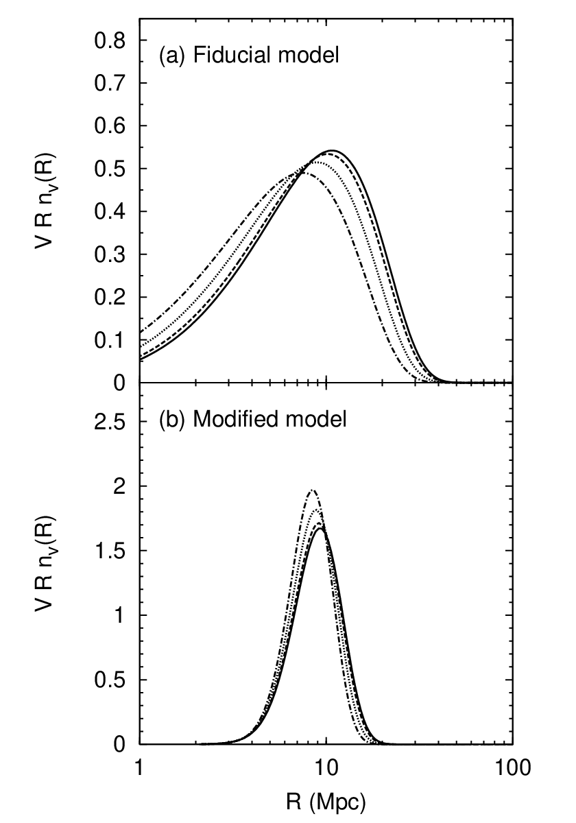
In what follows, we assume that a randomly chosen fraction of galaxies are LAEs. Mathematically, this decreases the mean observable galaxy density derived from LAE surveys by a factor , from now on referred to as the visible fraction. The observable mean galaxy density is given by
| (16) |
where is the intrinsic mean galaxy density and the superscript “o” denotes observable. The mean galaxy density within an underdense region decreases by the same factor .
The procedure for calculating void size distributions is only slightly modified from the usual case, because the halo mass threshold is now a function of . For a fixed observable mean galaxy density and visible fraction, equation (16) is solved for . As before, we define voids in terms of the observable mean galaxy underdensity through equation (3).
Figure 9 shows the void size distributions at for a variety of visible fractions in the fiducial model. Panel shows the modified model of §3.2. Both panels in Figure 9 show that the visible fraction has only a small effect on the void size distributions. Even under the assumption that 10% of LAEs emit, there is only a difference in characteristic scales with the fiducial curves, and even less with the modified model. The visible fraction does however have an important effect on the role of stochastic voids. Since we have held the observable galaxy number density fixed, the corresponding stochastic void distributions are unaffected by . Therefore, as decreases and the characteristic scales of real voids gets smaller, void samples are increasingly contaminated by stochastic fluctuations.
5 Comparison to Observations
Owing to a lack of statistics, a rigorous comparison of our calculations to observational surveys is not possible. In this section, we content ourselves with a rough comparison to the surveys of Shimasaku et al. 2006 and Ouchi et al. 2005. We focus on due to a number of recent claims of large-scale structure at this redshift.
Shimasaku et al. 2006 report evidence for the existence of large scale structure at in their photometric sample of 89 LAEs, including 34 spectroscopically confirmed objects. Their argument is based on a roughly 20 % overdensity and underdensity in the western and eastern halves of their sky distribution respectively. Their survey covers a continuous area of 725 arcmin2 and redshifts of , corresponding to a survey volume of . We find a volume filling fraction for voids with at least half of their survey volume and . The large volume filling fraction suggests that our result is consistent with the possibility that the observed underdense region in Shimasaku et al. 2006 is a void progenitor.
Ouchi et al. 2005 report much more well-defined large-scale structure. Their catalog of 515 LAEs at , which covers an area of 180 Mpc 180 Mpc 48 Mpc, exhibits a high degree of clustering. They find clearly defined voids and filamentary features. Moreover, the voids depicted in their survey are extremely large, ranging in size from 10 - 40 comoving Mpc in scale. Taking the scales of stochastic fluctuations and survey depth into account, these scales roughly correspond to void volumes of , where we have approximated them to be cylindrical regions with lengths of . A direct comparison of these voids to our predictions is problematic since our model assumes a spherical geometry. The best we can do is compare void volumes. The modified distribution shown in Figure 9 indicates that the voids of interest have a radii ranging from , or comoving volumes of . Although our modified definition yields volumes that are slightly smaller than the observed voids, the fiducial model in Figure 2 predicts the existence of a small number of larger scale voids with comoving diameters and volumes as high as and respectively. Thus, we do not consider the large voids observed by Ouchi et al. 2005 to be in contradiction with our results. Note as well that this model under-predicts the sizes of voids by a comparable amount (Furlanetto & Piran 2006); the discrepancy may be due to redshift space distortions, the non-spherical regions relevant to this narrow-band survey, or our simplified void identification algorithm.
Interestingly, the widest and most recent LAE survey conducted by Murayama et al. 2007 does not find convincing evidence for the clustering observed by Ouchi et al. 2005. Their survey consists of 119 LAE candidates in a 1.95 deg2 area, corresponding to a number density of . With such a small sky density (eight times smaller than Ouchi et al. 2005), true voids are masked by stochastic fluctuations (which have characteristic scales ).
Finally, we emphasize the difficulty in drawing conclusions from comparisons to sky distribution maps. Given the poor statistics, it is often difficult to determine conclusively whether a given empty region is a real void, and without redshifts we must compare our (spherical) predicted voids to cylindrical survey volumes. Furthermore, the samples we have described here are not completely spectroscopically confirmed and probably contain a reasonable fraction of low-redshift contaminants. When voids are defined based on only a few galaxies, such contamination can significantly affect the statistics (and, because the contaminants are also line-emitting galaxies at discrete redshifts, can introduce their own large-scale structure). At the very least, they affect the mass threshold of the survey (although probably not as much as uncertainty in ). Detailed comparisons will require simulations of the effects of these contaminants. The best we can say now is that there is no inconsistency with our model. Future surveys will undoubtedly allow for a more systematic comparison.
6 Discussion
We have calculated void size distributions at – using the excursion set model developed by Sheth & van de Weygaert 2004 and Furlanetto & Piran 2006. The latter found characteristic void radii of at . For the observational sensitivities assumed in this paper, we obtained characteristic void radii that are very similar: for redshifts between and . These results are virtually independent of the void-crushing barrier (for any reasonable choice). We have shown that characteristic void scales actually increase with redshift for a fixed halo mass threshold due to a decreased number density and increased bias with respect to the underlying matter density. Following recent studies on the abundances of low-redshift LAEs, we explored the possibility that only a fraction of galaxies are sampled in LAE surveys. This has only a small effect on the void size distribution but increases the contamination of void samples by stochastic fluctuations.
In section 3, we have explored stochastic fluctuations in the galaxy distribution. These fluctuations, although inherently different from the ”real” voids we model in this paper, will result in large empty regions in the sky. Stochastic voids can therefore contaminate real void samples and lead to erroneous conclusions on the formation of large-scale structure. We have estimated the typical scale of these regions to be slightly smaller than the characteristic scale of true voids at . At , the situation depends on the particular choice of . For , stochastic voids are typically the same scale as real voids. The increased importance of stochastic fluctuations will make the identification of large-scale structure at this redshift difficult. Attempts to do so must observe halos near the minimum mass to form stars, –, in order for true voids to dominate the observed distribution.
We found that a large fraction of real voids in our fiducial model contain no visible galaxies, adding to the difficulties in differentiating them from stochastic fluctuations. We have presented a modified definition of voids that incorporates both stochastic and real voids and so is easier to compare to the limited observational samples thus far available. In our new approach, we defined voids in terms of the probability for a region to be empty. We found that the modified void distributions are more sharply peaked and have characteristic scales that are comparable to the fiducial model.
We have also attempted to visually compare our results to the most recent narrow-band filter surveys at . While we found no inconsistencies, it is difficult to draw any decisive conclusions because of small-number statistics, projection effects, and lower-redshift contaminants. Obviously, a more systematic approach is required. Future surveys promise to provide better statistics and increased sample volumes for studies on high-redshift voids.
In the context of next generation surveys for high-redshift galaxies, our model is useful for gauging the impact of cosmic variance. Consider a fictitious survey at with a detection threshold of . Figure 6 illustrates that stochastic voids with will dominate the sky distribution. Therefore, one must either search for voids with or search deeper for significantly smaller sources. The latter may be possible if the sources observed by Stark et al. 2007 are indeed at , in which case they imply that halos near are visible (Mesinger & Furlanetto 2007). However, high-redshift galaxies are so highly biased that even with deep observations, a substantial fraction of the Universe is filled with empty or nearly-empty regions. For example, at and , of space is filled by regions that are at least 80% underdense in galaxies and at least 20 Mpc across – or fully 7 arcmin. With the small fields of view available to near-infrared detectors, this suggests that either many independent fields must be observed or a large contiguous volume surveyed to be guaranteed of detecting a reasonable number of sources.
Finally, we have neglected reionization and its effect on the appearance of large-scale structure. Regions of neutral hydrogen are expected to modulate the LAE density on large scales and accentuate the appearance of structure (Furlanetto et al. 2004; Furlanetto et al. 2006; McQuinn et al. 2006; McQuinn et al. 2007; Mesinger & Furlanetto 2007). Although the precise time frame is currently unknown, quasar observations and cosmic microwave background measurements have provided some evidence that reionization occurred between (e.g, Fan et al. 2006; Page et al. 2007; Mesinger & Haiman 2004; Mesinger & Haiman 2007). Interestingly, Kashikawa et al. 2006 found a significant high-luminosity suppression in the LAE luminosity function between and . Whether or not reioinization is responsible for this effect is currently unclear (Dawson et al. 2007, no such suppression was observed by).
Because IGM absorption modulates the LAE density on large scales, we would expect reionization to have a substantial effect on the observed void sizes in such narrow-band surveys (it should not affect galaxies identified through broadband effects). Of course, the plots in Figure 3 provide analytic estimates only of the intrinsic void size distributions. They provide a basis for comparison with high-redshift surveys in order to determine whether the observed features are easily attributable to the large-scale clustering alone. It therefore helps illuminate efforts to use voids to constrain the IGM properties during reionization, as first attempted by McQuinn et al. 2007.
References
- Benson et al. (2003) Benson A. J., Hoyle F., Torres F., Vogeley M. S., 2003, MNRAS, 340, 160
- Bond et al. (1991) Bond J. R., Cole S., Efstathiou G., Kaiser N., 1991, ApJ, 379, 440
- Casas-Miranda et al. (2002) Casas-Miranda R., Mo H. J., Sheth R. K., Boerner G., 2002, MNRAS, 333, 730
- Cohn & White (2007) Cohn J. D., White M., 2007, submitted to MNRAS (arXiv.org/0706.0208[astro-ph])
- Colberg et al. (2005) Colberg J. M., Sheth R. K., Diaferio A., Gao L., Yoshida N., 2005, MNRAS, 360, 216
- Conroy et al. (2005) Conroy C., Coil A. L., White M., Newman J. A., Yan R., Cooper M. C., Gerke B. F., Davis M., Koo D. C., 2005, ApJ, 635, 990
- Cuby et al. (2007) Cuby J.-G., Hibon P., Lidman C., Le Fèvre O., Gilmozzi R., Moorwood A., van der Werf P., 2007, A&A, 461, 911
- Dawson et al. (2007) Dawson S., Rhoads J. E., Malhotra S., Stern D., Wang J., Dey A., Spinrad H., Jannuzi B. T., 2007, submitted to ApJ (arXiv.org/0707.4182 [astro-ph]), 707
- de Lapparent et al. (1986) de Lapparent V., Geller M. J., Huchra J. P., 1986, ApJ, 302, L1
- Fan et al. (2006) Fan X., Strauss M. A., Becker R. H., White R. L., Gunn J. E., Knapp G. R., Richards G. T., Schneider D. P., Brinkmann J., Fukugita M., 2006, AJ, 132, 117
- Furlanetto et al. (2004) Furlanetto S. R., Hernquist L., Zaldarriaga M., 2004, MNRAS, 354, 695
- Furlanetto & Piran (2006) Furlanetto S. R., Piran T., 2006, MNRAS, 366, 467
- Furlanetto et al. (2006) Furlanetto S. R., Zaldarriaga M., Hernquist L., 2006, MNRAS, 365, 1012
- Gawiser et al. (2007) Gawiser E., et al., 2007, submitted to ApJ
- Gottlöber et al. (2003) Gottlöber S., Łokas E. L., Klypin A., Hoffman Y., 2003, MNRAS, 344, 715
- Gregory & Thompson (1978) Gregory S. A., Thompson L. A., 1978, ApJ, 222, 784
- Hoyle & Vogeley (2004) Hoyle F., Vogeley M. S., 2004, ApJ, 607, 751
- Hu et al. (2004) Hu E. M., Cowie L. L., Capak P., McMahon R. G., Hayashino T., Komiyama Y., 2004, AJ, 127, 563
- Jenkins et al. (2001) Jenkins A., Frenk C. S., White S. D. M., Colberg J. M., Cole S., Evrard A. E., Couchman H. M. P., Yoshida N., 2001, MNRAS, 321, 372
- Kashikawa et al. (2006) Kashikawa N., Shimasaku K., Malkan M. A., Doi M., Matsuda Y., Ouchi M., Taniguchi Y., Ly C., Nagao T., Iye M., Motohara K., Murayama T., Murozono K., Nariai K., Ohta K., Okamura S., Sasaki T., Shioya Y., Umemura M., 2006, ApJ, 648, 7
- Kirshner et al. (1981) Kirshner R. P., Oemler A., Schechter P. L., Shectman S. A., 1981, ApJ, 248, L57
- Lacey & Cole (1993) Lacey C., Cole S., 1993, MNRAS, 262, 627
- Mathis & White (2002) Mathis H., White S. D. M., 2002, MNRAS, 337, 1193
- McQuinn et al. (2005) McQuinn M., Furlanetto S. R., Hernquist L., Zahn O., Zaldarriaga M., 2005, ApJ, 630, 643
- McQuinn et al. (2007) McQuinn M., Hernquist L., Zaldarriaga M., Dutta S., 2007, MNRAS, 381, 75
- McQuinn et al. (2006) McQuinn M., Lidz A., Zahn O., Dutta S., Hernquist L., Zaldarriaga M., 2006, submitted to MNRAS (arXiv.org/0610094 [astro-ph])
- Mesinger & Furlanetto (2007) Mesinger A., Furlanetto S. R., 2007, submitted to MNRAS (arXiv.org/0708.0006 [astro-ph])
- Mesinger & Haiman (2004) Mesinger A., Haiman Z., 2004, ApJ, 611, L69
- Mesinger & Haiman (2007) Mesinger A., Haiman Z., 2007, ApJ, 660, 923
- Mo & White (1996) Mo H. J., White S. D. M., 1996, MNRAS, 282, 347
- Murayama et al. (2007) Murayama T., et al., 2007, ApJS, 172, 523
- Ota et al. (2007) Ota K., Iye M., Kashikawa N., Shimasaku K., Kobayashi M. A. R., Totani T., Nagashima M., Morokuma T., Furusawa H., Hattori T., Matsuda Y., Hashimoto T., Ouchi M., 2007, submitted to ApJ (arXiv.org/0707.1561 [astro-ph])
- Ouchi et al. (2005) Ouchi M., Shimasaku K., Akiyama M., Sekiguchi K., Furusawa H., Okamura S., Kashikawa N., Iye M., Kodama T., Saito T., Sasaki T., Simpson C., Takata T., Yamada T., Yamanoi H., Yoshida M., Yoshida M., 2005, ApJ, 620, L1
- Page et al. (2007) Page L., et al., 2007, ApJS, 170, 335
- Press & Schechter (1974) Press W. H., Schechter P., 1974, ApJ, 187, 425
- Sheth (1998) Sheth R. K., 1998, MNRAS, 300, 1057
- Sheth et al. (2001) Sheth R. K., Mo H. J., Tormen G., 2001, MNRAS, 323, 1
- Sheth & Tormen (1999) Sheth R. K., Tormen G., 1999, MNRAS, 308, 119
- Sheth & van de Weygaert (2004) Sheth R. K., van de Weygaert R., 2004, MNRAS, 350, 517
- Shimasaku et al. (2003) Shimasaku K., et al., 2003, ApJ, 586, L111
- Shimasaku et al. (2004) Shimasaku K., Hayashino T., Matsuda Y., Ouchi M., Ohta K., Okamura S., Tamura H., Yamada T., Yamauchi R., 2004, ApJ, 605, L93
- Shimasaku et al. (2006) Shimasaku K., Kashikawa N., Doi M., Ly C., Malkan M. A., Matsuda Y., Ouchi M., Hayashino T., Iye M., Motohara K., Murayama T., Nagao T., Ohta K., Okamura S., Sasaki T., Shioya Y., Taniguchi Y., 2006, PASJ, 58, 313
- Spergel et al. (2007) Spergel D. N., et al., 2007, ApJS, 170, 377
- Stark et al. (2007) Stark D. P., Ellis R. S., Richard J., Kneib J.-P., Smith G. P., Santos M. R., 2007, ApJ, 663, 10
- Vogeley et al. (1994) Vogeley M. S., Geller M. J., Park C., Huchra J. P., 1994, AJ, 108, 745
- Willis & Courbin (2005) Willis J. P., Courbin F., 2005, MNRAS, 357, 1348
- Zentner (2007) Zentner A. R., 2007, International Journal of Modern Physics D, 16, 763