On numerical averaging of the conductivity coefficient using two-scale extensions

Vsevolod Laptev¹¹ 1 This work was carried out during the tenures of a fellowship from University/ITWM in Kaiserslautern (Germany) and an ERCIM fellowship in Luxembourg and Norway. e-mail: laptevv@mail.ru

Abstract

In this article we compare solutions to elliptic problems having rapidly oscillated conductivity (permeability, etc) coefficient with solutions to corresponding homogenized problems obtained from two-scale extensions of the initial coefficient. The comparison is done numerically on several one and two dimensional test problems with randomly generated coefficients for different intensities of oscillation. The dependency of the approximation error on the size of averaging is investigated.

Key words. homogenization, averaging, non-periodic coefficients, elliptic equation, numerical micro-macro comparison

AMS subject classifications. 35B27,35B40,35J25,65N12,65N30

1 Introduction

We consider a second order elliptic equation with a rapidly oscillated coefficient $a_{M}(\cdot)$ :

-\nabla\cdot(a_{M}(x)\nabla u)=f\qquad\mbox{in $\Omega$,}\qquad u|_{\partial\Omega}=g.

(1)

The equation appears to describe such problems as the stationary heat transfer in composite materials, the flow in non-homogeneous porous media as well as in many others. For the periodic coefficient, the averaging procedure is well known and is called the periodic homogenization [1],[13],[17]. The general non-periodic case is very important for practical applications (e.g. in geoscience, petroleum engineering), and a vast literature exist discussing and comparing algorithms intended for averaging the permeability coefficient (see the reviews [5],[11],[15],[16]). Some algorithms are based on the idea that the effective (averaged, upscaled, equivalent grid block) permeability field in the whole domain can be determined by solving the flow problem locally [3]. They vary in the choices of the local subdomain, the boundary conditions, and the ways to extract the effective permeability coefficient from the solution of the local problem. These algorithms usually perform well, and intuitively there should be arguments to justify their usage.

An effective coefficient $A(\cdot)$ in the averaged problem

-\nabla\cdot(A(x)\nabla U)=f\qquad\mbox{in $\Omega$,}\qquad U|_{\partial\Omega}=g.

(2)

is generally different from $a_{M}(\cdot)$ , and the solution $U$ is different from $u$ . Therefore there is a trouble with perfect justification: the difference between these two solutions in some cases can be unacceptable. Homogenization is known as a rigorous way to justify an averaging process. This is so because homogenization deals with sequences, not with single problems. And if the sequence of problems converges in some sense to a limit problem then, whatever strict requirements we have, there is always a set of problems from the sequence for which this limit can be considered as an averaged problem. Although in practice we usually need to upscale a single problem like (1), not the whole sequence. Nevertheless, if our initial problem (1) belongs to the sequence in the homogenization process then the limit problem may be a reasonable candidate for upscaled initial problem, even if we cannot improve the approximation. We only need that the sequence is homogeneous in the sense that all its members, including our initial problem, have something in common (it is important to avoid situations when a convergent sequence contains an element which has nothing to do with the rest of the sequence).

One way to do so is to use the sequence from locally periodic homogenization (see e.g.[1, p.71])

-\nabla\cdot\left(a\left(x,\frac{x}{\varepsilon}\right)\nabla u_{\varepsilon}\right)=f\qquad\mbox{in $\Omega$,}\qquad u_{\varepsilon}|_{\partial\Omega}=g,

(3)

where the function $a(x,y)$ is a two-scale extension of the initial coefficient $a_{M}(\cdot)$ :

Definition 1.1 (from [8]).

Let us say that a function $a(x,y)$ , $(x,y)\in\Omega\times\mathbb{R}^{d}$ , $1$ -periodic in the variable $y$ , is a two–scale extension for $a_{M}(x)$ if there exists a positive number $\bar{\varepsilon}$ such that

a\left(x,\frac{x}{\bar{\varepsilon}}\right)=a_{M}(x),\qquad\forall x\in\Omega.

(4)

Having a two-scale extension, we can choose a strictly positive sequence $\{\varepsilon_{n}\}\to 0$ , containing $\bar{\varepsilon}$ , and consider (3) with $\varepsilon$ from $\{\varepsilon_{n}\}$ as a sequence in the scope of locally periodic homogenization. The expressions for $A(x)$ and corrections of $U$ can be found in the literature devoted to homogenization. All the members in the sequence (3) have in common the function $a(x,y)$ ; and at $\varepsilon=\bar{\varepsilon}$ we recover the initial problem (1). In this sense a two-scale extension establishes a connection between (2) calculated from the homogenization algorithm, and the initial problem (1). As it was already mentioned, we cannot claim that (2) with such $A(\cdot)$ is the averaged problem for (1). Moreover, there are (infinitely) many two-scale extensions leading to different $A(\cdot)$ for the same $a_{M}(\cdot)$ . Nevertheless, we expect that among them there could be classes of extensions appropriate for averaging. Therefore it is interesting to test numerically the two-scale extensions from [8] on several model problems with non-periodic coefficients. In each test we calculate both the solution $u$ and the (corrected) solution $U$ and verify whether the solutions are close to each other in any sense. Such numerical evidence could give an idea about the areas of applicability (if any) of the approach.

The article is organized as follows. In the next section several ways to construct two–scale extension for arbitrary initial coefficients $a_{M}(x)$ are presented. The section 3 contains cell problems and averaging algorithms from the homogenization theory. Section 4 consists of numerical results in 1D for ${\mathcal{C}}$ and ${\mathcal{D}}_{k}$ extensions (Subsection 4.2), and ${\mathcal{D}}_{2}$ -extension in 2D (Subsection 4.3).

2 Two-scale extensions

The two-scale extensions (which we numerically investigate in this article) and their properties were presented and discussed in [8].

The trivial extension is given by $a(x,y)=a_{M}(x)$ . More useful extensions can be constructed in the following way (assuming that $a_{M}(x)$ is known in a larger domain $\widetilde{\Omega}\supset\Omega$ in order to avoid uncertainties close to $\partial\Omega$ ):

•

we choose $\bar{\varepsilon}>0$ (small in comparison to the typical size of $\Omega$ );
•
for each $x\in\Omega$ we choose an $\bar{\varepsilon}$ -cube $W_{x}$ with sides aligned with the coordinate axes, containing $x$ : $x\in W_{x}$ . We also assume that $\widetilde{\Omega}$ is large enough: $W_{x}\subset\widetilde{\Omega}$ , $\forall x\in\Omega$ ( $W_{x}$ is a cubic ”Representative Elementary Volume” around $x$ , $\bar{\varepsilon}$ is a size of averaging).
It is reasonable to distinguish two main choices of $W_{x}$ ( ${\mathcal{C}}$ – continuous, ${\mathcal{D}}$ – discrete):
- ( ${\mathcal{C}}$ )
  
  $W_{x}$ is an $\bar{\varepsilon}$ -cube with the center $x$ ;
- ( ${\mathcal{D}}$ )
  
  Having a partition $\overline{\Omega}=\bigcup_{j=1}^{N_{\mathcal{D}}}\overline{\Omega_{j}}$ ( $\Omega_{i}\cap\Omega_{j}=\emptyset$ , $i\neq j$ ) that each $\Omega_{j}$ has an $\bar{\varepsilon}$ -cube $W_{j}$ ( $\Omega_{j}\subseteq W_{j}$ , $\hat{x}_{j}$ is a center of $W_{j}$ ) then for each $x\in\Omega_{j}$ we can define $W_{x}:=W_{j}$ .

Now we fix $x\in\Omega$ and construct $a(x,\cdot)$ :

1.

$\tilde{a}(x,y)=a_{M}(y)$ , $y\in W_{x}$ ;
2.

$\tilde{a}(x,y)$ is extended $\bar{\varepsilon}$ -periodically in $y$ to the whole space $\mathbb{R}^{d}$ ;
3.

$a(x,y)=\tilde{a}(x,\bar{\varepsilon}y)$ is the two-scale extension.

Depending on the choice of $W_{x}$ we have ${\mathcal{C}}$ -extensions and ${\mathcal{D}}$ -extensions.

Remark 2.1.

The function $a(x,y)$ is still a two-scale extension if we substitute the item 1. above by one of the following more weak requirements:

•

$\tilde{a}(x,y)=a_{M}(y)$ , $y\in O(x)\subseteq W_{x}$ , where $O(x)$ is a neighbourhood of $x$ ;
•

$\tilde{a}(x,y)=a_{M}(y)$ , $y=x$ ;

and let $\tilde{a}(x,y)$ to be free in the rest of $W_{x}$ .

This can be used to modify the coefficient near the boundary of $W_{x}$ e.g. if we want $a(x,y)$ to be continuous. The second requirement is so weak that it allows to construct any two-scale extension satisfying Def.1.1 (without saying how to do it). Probably we should have something like $\tilde{a}(x,y)\approx a_{M}(y)$ , $y\in O(x)$ not to loose the relation between $a_{M}(\cdot)$ and $a(\cdot,\cdot)$ completely. Anyway, we don’t consider these possibilities further in this paper.

The ${\mathcal{D}}$ -extension depends on the choice of $\{\Omega_{j}\}$ . If we are going to solve (2) using an unstructured grid then $\{\Omega_{j}\}$ could be chosen related to that grid. For example, if we deal with FEM then each $\Omega_{j}$ could be a union of one or more finite elements. Here we will test only one kind of a subdivision of $\Omega$ into $\{\Omega_{j}\}$ , which is more appropriate for solving (2) on Cartesian grids:

Definition 2.1.

Let $k\geq 1$ , $\bar{\varepsilon}>0$ be given. We divide $\mathbb{R}^{d}$ into cubes

\Box_{I}=\Bigl(i_{1}h,(i_{1}+1)h\Bigr)\times\dots\times\Bigl(i_{d}h,(i_{d}+1)h\Bigr),\qquad h=\bar{\varepsilon}/k,\quad I=(i_{1},\dots,i_{d})\in\mathbb{Z}^{d}.

We set $\Omega_{j}=\Box_{I(j)}\cap\Omega$ , where $I(j)$ is some numeration of those cubes which have a non-empty intersection with $\Omega$ , $j=1,\dots,N_{\mathcal{D}}$ . $W_{j}$ is a cube with the side $\bar{\varepsilon}=kh$ , and the center at the same point as the center of $\Box_{I(j)}$ . The ${\mathcal{D}}$ -extension constructed this way let us call a ${\mathcal{D}}_{k}$ -extension.

3 Averaging using two-scale extension

The sequence (3) is well investigated in the homogenization theory. It is known that the averaged coefficient $A(x)$ at $x\in\Omega$ in the limit problem (2) can be calculated via a so-called cell problem. Next we remind different formulations of the cell problem applied to the two-scale extensions from Section 2. Let us fix an arbitrary $x\in\Omega$ .

Differential form in $\mathbb{R}^{d}$ :

\left\{\begin{array}[]{l}-\nabla_{y}\cdot\Bigl(a(x,y)\bigl(\nabla_{y}w_{j}(x,y)+e_{j}\bigr)\Bigr)=0\qquad\mbox{in $\mathbb{R}^{d}$}\\ \int\limits_{Y}w_{j}(x,y)\,dy=0,\qquad\mbox{$w_{j}(x,y)$ is $1$-periodic in $y$}.\end{array}\right.

(5)

Differential form in $Y$ .

Since we prefer to solve the problems in a bounded domain, we can rewrite them in a differential form in a cube $Y=(0,1)^{d}$ :

\left\{\begin{array}[]{l}-\nabla_{y}\cdot\Bigl(a(x,y)\bigl(\nabla_{y}w_{j}(x,y)+e_{j}\bigr)\Bigr)=0\qquad\mbox{in Y}\\ \mbox{Boundary conditions on $S^{0}_{i}$,$S^{1}_{i}$ for all $i=1,\dots,d$}:\\ w_{j}(x,\cdot)|_{S^{0}_{i}}=w_{j}(x,\cdot)|_{S^{1}_{i}}\\ e_{i}\cdot\bigl(a(\nabla_{y}w_{j}+e_{j})\bigr)(x,\cdot)|_{S^{0}_{i}}=e_{i}\cdot\bigl(a(\nabla_{y}w_{j}+e_{j})\bigr)(x,\cdot)|_{S^{1}_{i}}\\ \int\limits_{Y}w_{j}(x,y)\,dy=0\end{array}\right.

(6)

where $S^{\alpha}_{i}=\{y\in\overline{Y}:y_{i}=\alpha\}$ . $w_{j}(x,\cdot)$ is extended periodically in $y$ from $Y$ to $\mathbb{R}^{d}$ .

Variational form:

find $w_{j}(x,\cdot)\in H^{1}_{per}(Y)/\mathbb{R}$ such that

\int_{Y}\nabla_{y}\phi(y)^{T}a(x,y)\nabla_{y}w_{j}(x,y)\,dy=-\int_{Y}\nabla_{y}\phi(y)^{T}a(x,y)e_{j}\,dy\qquad\forall\phi\in H^{1}_{per}(Y)/\mathbb{R}.

(7)

The averaged coefficient $A(x)$ can be calculated from the solutions $w_{j}$ , $j=1,\dots,d$ :

A_{ij}(x)=\int_{Y}e_{i}^{T}a(x,y)\Bigl(\nabla_{y}w_{j}(x,y)+e_{j}\Bigr)\,dy.

(8)

After solving (2), the solution $U$ could be corrected (see e.g. [1, p.76]):

\widehat{U}(x)=U(x)+\bar{\varepsilon}\sum_{j=1}^{d}w_{j}\left(x,\frac{x}{\bar{\varepsilon}}\right)\frac{\partial U}{\partial x_{j}}(x).

(9)

Roughly speaking, $\widehat{U}$ approximates $u$ from (1) itself, and $U$ approximates the averaged $u$ .

Due to $1$ -periodicity of $w_{j}(x,y)$ in $y$ , we can substitute $Y$ in (6)-(8) by any other $1$ -cube $C=(c^{1}_{min},c^{1}_{min}+1)\times\dots\times(c^{d}_{min},c^{d}_{min}+1)$ . $S^{\alpha}_{i}$ we can redefine as $\{y\in\overline{C}:y_{i}=c^{i}_{min}+\alpha\}$ . For practical purposes it is convenient to take $C=Y_{x}$ , where $Y_{x}=\{y\in\mathbb{R}^{d}\mid\bar{\varepsilon}y\in W_{x}\}$ for each fixed $x\in\Omega$ . Then for $y\in Y_{x}$ we have $a(x,y)=\tilde{a}(x,\bar{\varepsilon}y)=a_{M}(\bar{\varepsilon}y)$ . It is also useful for calculating the correction (9) since $x$ being (always) inside $W_{x}$ implies $x/\bar{\varepsilon}\in Y_{x}$ . Thus, we don’t need to store $a(\cdot,\cdot)$ as a function of $d\times d$ variables – it is possible to obtain all necessary information directly from $a_{M}(\cdot)$ . The averaging method is local: the averaged coefficient $A(x)$ and $w_{j}(x,\cdot)$ depend only on the values of $a_{M}(\cdot)$ in $W_{x}$ , a neighbourhood of $x$ .

$W_{x}$ in the ${\mathcal{C}}$ -extension is changing with the point $x$ ; the field $A(\cdot)$ is a result of solving the cell problems at all points from $\Omega$ . This is different from the ${\mathcal{D}}$ -extension, where a finite number of cell problems has to be solved since $W_{x}$ is the same in $\Omega_{j}$ ( $W_{x}=W_{j}$ ). In this case $A(x)$ has a constant value in each $\{\Omega_{j}\}$ . We note, that the averaged coefficients from both ${\mathcal{C}}$ and ${\mathcal{D}}$ extensions coinside at the points $\hat{x}_{j}$ , the centers of $W_{j}$ . We also know that $A(x)$ from the ${\mathcal{C}}$ -extension should be continuous ([8, Prop. 7.1]). Therefore from a practical point of view these extensions could be seen as different interpretations of the coefficient $A(x)$ known at the finite number of points $\hat{x}_{j}$ : we can treat the data as a continuous or a piecewise constant function. The continuous data can be interpolated in space between $\hat{x}_{j}$ . The interpolation makes possible the numerical averaging with ${\mathcal{C}}$ -extensions. Such averaging needs additional care comparing to the averaging from ${\mathcal{D}}$ -extensions: if the distribution of $\hat{x}_{j}$ is not dense enough in $\Omega$ , the interpolated field could be significantly different from the exact $A(\cdot)$ (e.g. by missing oscillations).

Remark 3.1.

The ${\mathcal{D}}_{k}$ -extension, (6), (8) lead to the averaging algorithm for $A(x)$ proposed in [14, p. 527] as one of several alternative upscaling procedures using ”border regions”. The early algorithm [3] can be obtained from the ${\mathcal{D}}_{1}$ -extension (where $W_{j}=\Omega_{j}$ ).

Remark 3.2.

The corrected approximation $\widehat{U}$ , calculated from a ${\mathcal{D}}$ -extension via (9), is not continuous. The jumps on $\overline{\Omega}_{n}\cap\overline{\Omega}_{m}$ are expected due to the abrupt change of the cell solutions $w_{j}$ when $x$ goes from $\Omega_{n}$ to $\Omega_{m}$ . These jumps are more significant for ${\mathcal{D}}_{k}$ -extensions with smaller $k$ since for large $k$ , $W_{n}$ and $W_{m}$ have a large common volume. Here it creates no problem since we use only $L^{2}$ , $L^{\infty}$ norms for the comparison $\widehat{U}$ with $u$ . Although if one is interested in fluxes or $H^{1}$ approximations then the correction in the form (9) is probably a bad choice.

4 Numerical results

Our main purpose in this section is to solve several model problems (1), (2) semi-analytically (if possible) or numerically and to compare $u$ with $U$ and $\widehat{U}$ .

4.1 Random number generator

In most of the numerical examples in this article the coefficient $a_{M}(\cdot)$ is defined with the help of a random sequence $\{\xi_{i}\}$ . To generate the sequence $\{\xi_{i}\}$ of real numbers we read at each occasion an $i$ -th pair $(b_{0},b_{1})$ of bytes from the file [6] ( $b_{0},b_{1}\in\mathbb{Z_{+}}$ , $0\leq b_{0},b_{1}\leq 255$ ) and calculate

\xi_{i}=(b_{0}+b_{1}2^{8})/(2^{16}-1),\qquad\xi_{i}\in[0,1],\quad i=1,2,\dots\quad.

The first five pairs are $(34,178)$ , $(52,184)$ , $(220,178)$ , $(237,13)$ , $(19,247)$ . This approach was chosen since it is easy to reproduce the sequence on different computer platforms.

4.2 1D tests

In 1D we have the following problem

\frac{d}{dx}\left(a(x)\frac{du}{dx}\right)=f(x),\qquad u(0)=u_{l},\quad u(1)=u_{r},

where $a(x)$ is either the initial coefficient $a_{M}(x)$ or the averaged coefficient $A(x)$ . $a_{M}(x)$ is a constant in $[0,1/4)\cup(3/4,1]$ and has oscillations in $[1/4,3/4]$ (see Fig.1–3). The solution to the equation can be written analytically:

a(x)u^{\prime}(x)=C+\int_{0}^{x}f(x)\,dx=C+F(x),\qquad u^{\prime}(x)=\frac{C}{a(x)}+\frac{F(x)}{a(x)},

(10)

u(x)=u_{l}+C\int_{0}^{x}\frac{1}{a(x)}\,dx+\int_{0}^{x}\frac{F(x)}{a(x)}\,dx,

where $C$ can be determined from the boundary condition $u(1)=u_{r}$ :

C=\left(\int_{0}^{1}\frac{1}{a(x)}\,dx\right)^{-1}\left(u_{r}-u_{l}-\int_{0}^{1}\frac{F(x)}{a(x)}\,dx\right).

Thus, the semi-analytical numerical solutions for initial and averaged problems need only the numerical integration. It seems to be more flexible not to consider $a(\cdot)$ in some exact analytical form, but to use discretizations of $a(x)$ , $u(x)$ on uniform grids. Thanks to one-dimensionality, grids with millions of points are available ( $N_{sol}$ – number of points).

The cell problem ( $x$ is like a parameter here)

\frac{d}{dy}\left(a(x,y)\Bigl(\frac{dw(x,y)}{dy}+1\Bigr)\right)=0,\qquad w(x,0)=w(x,1)

also can be solved analytically (up to an additive constant):

\frac{dw(x,y)}{dy}=\frac{C(x)}{a(x,y)}-1,\qquad w(x,y)=w(x,0)+C(x)\int_{0}^{y}\frac{dy}{a(x,y)}-y,

where $C(x)=\Bigl(\int_{0}^{1}a(x,y)^{-1}\,dy\Bigr)^{-1}$ , since $w(x,0)=w(x,1)$ . The averaged coefficient is

A(x)=\int_{0}^{1}a(x,y)\left(\frac{dw(x,y)}{dy}+1\right)\,dy=C(x),

A(x)=\left(\int_{0}^{1}\frac{dy}{\tilde{a}(x,\bar{\varepsilon}y)}\right)^{-1}=\left(\frac{1}{\bar{\varepsilon}}\int_{0}^{\bar{\varepsilon}}\frac{dz}{\tilde{a}(x,z)}\right)^{-1}=\left(\frac{1}{\bar{\varepsilon}}\int_{w_{-}(x)}^{w_{+}(x)}\frac{dz}{a_{M}(z)}\right)^{-1},

where $W_{x}=(w_{-}(x),w_{+}(x))=(\hat{x}(x)-\bar{\varepsilon}/2,\hat{x}(x)+\bar{\varepsilon}/2)$ . For the ${\mathcal{C}}$ -extension: $\hat{x}(x)=x$ . For the ${\mathcal{D}}_{k}$ -extension: $\hat{x}(x)=h(\lfloor x/h\rfloor+0.5)$ , where $\lfloor y\rfloor$ is the largest number from $\mathbb{Z}$ : $\lfloor y\rfloor\leq y$ .

The $H^{1}$ correction (9) is

\widehat{U}(x)=U(x)+\bar{\varepsilon}U^{\prime}(x)w(x,x/\bar{\varepsilon}),

where the expression for $U^{\prime}(x)$ can be found in (10).

Remark 4.1.

The harmonic averaging is used in the finite volume method e.g. for discretizing the elliptic operator with discontinuous coefficients [12].

Refer to caption — Figure 1: $a_{M}(\cdot)$ for $\epsilon=0.004$ (case a1)

For the 1D tests the coefficient $a_{M}(x)$ in $\tilde{\Omega}=(-1,2)$ is

a_{M}(x)=\left\{\begin{array}[]{cl}1&x\in(-1,1/4)\cup[x_{M},2)\\ 0.001+\xi_{2i}&x\in[x_{i},x_{i+1}),\quad i=1,\dots,M-1\\ \end{array},\right.

where

x_{1}=\frac{1}{4},\quad x_{i+1}=x_{i}+\epsilon\frac{(0.1+4\xi_{2i-1})}{2.1},\quad x_{M-1}<\frac{3}{4}\leq x_{M},

$\{\xi_{i}\}$ is the pseudo-random sequence of numbers, $\epsilon$ is either $0.004$ (case a1, see Fig.1), $0.001$ (case a2, see Fig.2) or $0.00025$ (case a3, see Fig.3). The homogeneous boundary conditions $g\equiv 0$ ( $u_{l}=u_{r}=0$ ) are chosen. We use three different r.h.s.: oscillating, constant and discontinuous.

f(x)=\left\{\begin{array}[]{cl}50\sin(30x)&\mbox{case f1}\\ -4&\mbox{case f2}\\ 4\bigl(\mathbf{1}_{(1/2,3/4)}-\mathbf{1}_{(1/4,1/2)}\bigr)&\mbox{case f3}\\ \end{array}\right.,

where $\mathbf{1}_{(a,b)}(x)$ is a characteristic function of $(a,b)$ .

Let us look at one test more precisely. In Fig.4 the averaged coefficient for the case a2, obtained from ${\mathcal{C}}$ -extension for $\bar{\varepsilon}=0.016$ , is plotted. From Fig.5, where $U$ , $\widehat{U}$ and $u$ are compared, we see that the averaging is capable to provide good approximations, and that the correction $\widehat{U}$ approximates $u$ with a better quality than $U$ (the later looks more like an average of $u$ smoothing the abrupt curve).

To estimate quantitatively the quality of the approximation we will use:

\widehat{E}_{2}=\|\widehat{U}-u\|_{L^{2}(0,1)},\qquad\widehat{E}_{\infty}=\|\widehat{U}-u\|_{L^{\infty}(0,1)},\qquad E_{2}=\|U-u\|_{L^{2}(0,1)},\qquad E_{\infty}=\|U-u\|_{L^{\infty}(0,1)}.

4.2.1 ${\mathcal{C}}$ -extensions in 1D

In the first series of tests we solve the problems (1),(2) for different $a_{M}(\cdot)$ and $f(\cdot)$ (cases a2f1, a2f2, a2f3, a1f1, a3f1). The averaged coefficients are calculated from the ${\mathcal{C}}$ -extensions for different $\bar{\varepsilon}$ . The approximation errors are plotted in Fig.6–10. In all cases the uniform grids have $N_{sol}=8\cdot 10^{6}$ , $16\cdot 10^{6}$ , $32\cdot 10^{6}$ , $64\cdot 10^{6}$ number of points. We can see from the figures, that $\widehat{E}_{2}$ , $\widehat{E}_{\infty}$ curves for different $N_{sol}$ are splitted at the end ( $\bar{\varepsilon}\sim 10^{-4}$ ). Rounding errors and insufficient resolution could probably explain this, since the curve obtained on the coarsest grid $N_{sol}=8\cdot 10^{6}$ starts to deviate first, and the curve from the finest grid $N_{sol}=64\cdot 10^{6}$ remains longer close to the extrapolated line. The numerical results show that smaller $\bar{\varepsilon}$ lead to more accurate approximations, and that $\widehat{U}$ approximates $u$ better than $U$ does. The curves on some intervals look like straight lines (especially $\widehat{E}_{2}$ ). The slopes of the lines on the log-log plots give an idea about the order of convergence.

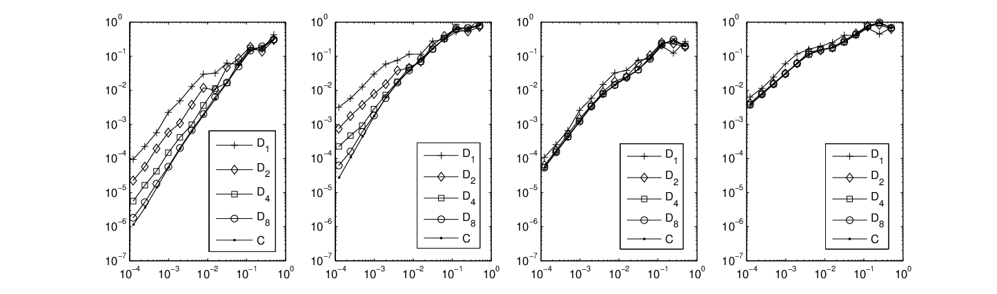
4.2.2 ${\mathcal{C}}$ -extensions and ${\mathcal{D}}_{k}$ -extensions in 1D

Calculation of the coefficient $A(\cdot)$ from a ${\mathcal{C}}$ -extension needs high computational resources (due to the fine grid), since the fine scale details of the averaged coefficient (see Fig.4) could disappear after interpolation of a coarse grid data. Opposite to that, the averaged coefficient from a ${\mathcal{D}}$ -extension is free from the interpolation error, and the needed computational resources are limited by the particular choice of the extension. Let us compare the qualities of approximation from ${\mathcal{C}}$ , ${\mathcal{D}}_{k}$ -extensions for $k=1,2,4,8$ . The grid has $N_{sol}=64\cdot 10^{6}$ nodes. From Fig.11 we see that the ${\mathcal{C}}$ -extension provides better $\widehat{U}$ approximations (possibly with higher order of convergence), although there is no significant difference when $U$ is concerned. We also observe that the quality of approximation from the ${\mathcal{D}}_{k}$ -extensions approach the quality of approximation from the ${\mathcal{C}}$ -extension when $k$ increases.

The (semi)-analytical solutions $U$ , $U^{\prime}$ , $\widehat{U}$ were used also for the ${\mathcal{D}}_{k}$ -extensions. This means that the errors which would appear in practical situation ( $U_{h}$ , $U_{h}^{\prime}$ instead of $U$ , $U^{\prime}$ ) were excluded here.

4.3 2D tests

1D case is very favorable for investigations: extremely fine grids and analytical expressions for the solutions are available. In 2D we are much more limited in means: we have no analytical solution for more or less realistic problem specification, and the finest grid for calculating numerical solutions contains only few thousand nodes discretizing OX,OY directions (here the maximum is $4096$ ). Appearance of arbitrary directions makes the difference from the 1D case.

A reliable investigation of the ${\mathcal{C}}$ -extension remains practically out of reach here. Thus, we restrict ourselves to ${\mathcal{D}}_{k}$ -extensions for $k=2$ . The extension has one parameter – $\bar{\varepsilon}$ . We also use the equivalent parameter $h=\bar{\varepsilon}/k=\bar{\varepsilon}/2$ emphasizing that the matrix valued coefficient $A(\cdot)$ is a piecewise constant function on the $h$ -grid. A coarser grid cannot resolve the coefficient properly.

The domain for 2D tests is $\Omega=(0,1)^{2}$ . The right hand side and the boundary values for (1), (2) are fixed for all tests: $f(x)\equiv 10$ in $\Omega$ , $g\equiv 0$ on $\partial\Omega$ . The coefficients $a_{M}(\cdot)$ are described below. We choose only infinitely smooth coefficients to optimize the accuracy of the numerical method on available grids. $a_{M}(\cdot)$ can be naturally extended from $\Omega$ to any $\widetilde{\Omega}\subset\mathbb{R}^{2}$ .

To solve the 2D elliptic problems with tensor coefficients (fine scale problem (1), homogenized problem (2), cell problems (7)) we divide the domain $(0,1)^{d}$ by a uniform Cartesian grid into $N\times N$ squares with the side $h=1/N$ ( $h$ -grid). All squares are subdivided into two triangles by the same diagonal, and the standard finite element method with linear base functions on such triangulation is used to solve the problems numerically. The coefficient is forced to have a constant value inside each square by taking the value in the center of the square for the whole square (such approximations are used for (1), (7) since the initial coefficients $a_{M}(\cdot)$ are smooth in our tests).

The averaged coefficient which is actually used to solve (2) numerically is different from the exact $A(\cdot)$ due to errors of approximation introduced while solving the cell problems on $N_{c}\times N_{c}$ grids. Let us call it $A_{h,h_{c}}(\cdot)$ instead of $A(\cdot)$ . The first index $h$ emphasizes that the coefficient is piecewise constant on the $h$ -grid, and the second index $h_{c}=1/N_{c}$ specifies the discretization step used to solve the cell problems. $N_{c}$ is independent from $N=1/h$ and should be large enough for solving cell problems with enough accuracy. In the tests described below, $N_{c}$ was usually chosen as large as possible under a constrain of reasonable total time of solving $N^{2}$ cell problems on a single processor computer. In addition, the grid $(NN_{c}/k)\times(NN_{c}/k)$ ( $k=2$ here) was fine enough for resolving all oscillations of $a_{M}(\cdot)$ in $\Omega$ . In some cases $A_{h,h_{c}}$ was compared with $A_{h,2h_{c}}$ , and the solutions of (2) with both $A_{h,h_{c}}$ and $A_{h,2h_{c}}$ were compared with each other in order to verify how the error in $A(\cdot)$ affects the accuracy.

The problem (2) with the coefficient $A_{h,h_{c}}(\cdot)$ we solve numerically on two grids: $h$ -grid and $h/4$ -grid. The solutions are $U_{h}$ and $U_{h,4}$ respectively. $U_{h}$ is cheap and therefore appropriate for solving practical problems, although the (coarsest possible) $h$ -grid cannot guarantee that $U_{h}$ is a good approximation for $U$ . For example, the difference between $U_{h}$ and $U_{h,4}$ is important when $A_{h,h_{c}}(\cdot)$ has a high contrast. Thus, we need also $U_{h,4}$ – our numerical substitute for $U$ .

In order to construct the numerical corrections $\widehat{U}_{h}$ , $\widehat{U}_{h,4}$ approximating $\widehat{U}$ from (9) we need to save the solutions of the cell problems. Since the computer memory is also a limited resource, the cell problem could be solved on $N_{c}\times N_{c}$ grid, but saved on $N_{cs}\times N_{cs}$ grid for $N_{cs}\leq N_{c}$ . And we need to store the values of $w_{j}$ only at the points which correspond to $\Omega_{i}$ inside $W_{i}$ . For example, we can choose a priory a set of points $\{x_{k}\}$ in $\Omega$ where we would like to know $\widehat{U}$ , and store the interpolated cell solutions from $W_{i}$ only at the points corresponding to $x_{k}\in\Omega_{i}$ . The derivatives from $U$ in (9) are approximated in the centers of $h$ squares via central differences and then interpolated in $\Omega$ . The values in the central differences are either from $U_{h}$ or from the projection $U_{h,4}$ to the $h$ -grid.

The following relative errors are used to compare the numerical solutions with the reference solution:

E_{2}(y)=\|y-u_{ref}\|_{L^{2}(\Omega)}/\|u_{ref}\|_{L^{2}(\Omega)},\quad E_{\infty}(y)=\|y-u_{ref}\|_{L^{\infty}(\Omega)}/\|u_{ref}\|_{L^{\infty}(\Omega)},

where the reference solution $u_{ref}$ is a numerical solution of (1) obtained on the finest grid $N_{ref}\times N_{ref}$ . $N_{ref}$ is either $2048$ or $4096$ depending on the intensity of oscillations in $a_{M}(\cdot)$ .

Each Fig.12,17–20 consists of two subfigures with $E_{2}$ (left) and $E_{\infty}$ (right) error functions. On each subfigure there are 3 functions: $c_{1}(h)$ , $c_{2}(h)$ , $c_{3}(h)$ . The markers correspond to all test cases.

$c_{1}$

The curves with square markers represent the functions $c_{1}(h)=E_{2}(u_{h})$ for the left subfigure, and $c_{1}(h)=E_{\infty}(u_{h})$ for the right subfigure, where $u_{h}$ is the numerical solution of (1) obtained on the $h$ -grid without averaging. $u_{h}$ on the finest grid is the reference solution $u_{ref}$ and therefore the corresponding square markers for $E_{2}(u_{ref})=E_{\infty}(u_{ref})=0$ are excluded from the curves.
$c_{2}$

The curves with circles represent the functions $c_{2}(h)=E_{2}(\widehat{U}_{h})$ for the left subfigure, and $c_{2}(h)=E_{\infty}(\widehat{U}_{h})$ for the right subfigure.
$c_{3}$

The curves with point markers represent the functions $c_{3}(h)=E_{2}(\widehat{U}_{h,4})$ for the left subfigure, and $c_{3}(h)=E_{\infty}(\widehat{U}_{h,4})$ for the right subfigure. The averaged coefficient is the same as for $c_{2}$ – $A_{h,h_{c}}(\cdot)$ , but $c_{3}$ is different from $c_{2}$ .

4.3.1 Test with explicitly given coefficient

In [10] the following coefficient for (1) was proposed as a test ”without scale separation”:

a_{M}(x_{1},x_{2})=\frac{1}{6}\left(\frac{1.1+\sin(2\pi x_{1}/\varepsilon_{1})}{1.1+\sin(2\pi x_{2}/\varepsilon_{1})}+\frac{1.1+\sin(2\pi x_{2}/\varepsilon_{2})}{1.1+\cos(2\pi x_{1}/\varepsilon_{2})}+\frac{1.1+\cos(2\pi x_{1}/\varepsilon_{3})}{1.1+\sin(2\pi x_{2}/\varepsilon_{3})}+\right.

\left.+\frac{1.1+\sin(2\pi x_{2}/\varepsilon_{4})}{1.1+\cos(2\pi x_{1}/\varepsilon_{4})}+\frac{1.1+\cos(2\pi x_{1}/\varepsilon_{5})}{1.1+\sin(2\pi x_{2}/\varepsilon_{5})}+\sin(4x_{1}^{2}x_{2}^{2})+1\right).

where $\varepsilon_{1}=1/5$ , $\varepsilon_{2}=1/13$ , $\varepsilon_{3}=1/17$ , $\varepsilon_{4}=1/31$ , $\varepsilon_{5}=1/65$ .

The curves $c_{1}$ , $c_{2}$ , $c_{3}$ for this test are plotted in Fig.12.

4.3.2 Tests with randomly constructed coefficients

Let us consider the scalar coefficient $a_{M}(x)=10^{\beta S(x)}$ , where

S(x)=\sum_{i=1}^{N_{\sin}}\sin\bigl(\pi i(x_{1}\sin(\psi_{i})+x_{2}\cos(\psi_{i})+\phi_{i})\bigr),\qquad\psi_{i}=2\pi\xi_{2i-1},\quad\phi_{i}=2\xi_{2i}\quad\beta=\frac{\log_{10}(C)}{M-m},

$\{\xi_{i}\}$ is the pseudo-random sequence of numbers, the constants $m$ , $M$

\begin{array}[]{ccccc}N_{\sin}&64&128&256&512\\ m&-19.7229&-36.1412&-49.6262&-81.8554\\ M&22.5351&34.124&51.5507&75.7885\end{array}

give approximations to minimum and maximum values of $S(x)$ in $\Omega$ respectively. This allows us to choose the constant $C=10^{4}$ as the contrast for $a_{M}(\cdot)$ ( $C\approx\max_{x}a_{M}(x)/\min_{x}a_{M}(x)$ ).

We use 4 different coefficients $a_{M}(\cdot)$ with different intensities of oscillation: $N_{\sin}=64$ , $128$ , $256$ , $512$ (see Fig.13). From this series we can observe what happens when $a_{M}(\cdot)$ becomes more and more oscillatory, and guess further behaviour towards more realistic situations. One test case ( $N_{\sin}=256$ , $h=1/16$ ) is illustrated in Fig.14,15 (see also [9], where similar results for another $a_{M}(\cdot)$ were presented). The curves $c_{1}$ , $c_{2}$ , $c_{3}$ are plotted in Fig.17– Fig.20. The contrast of the averaged coefficient is presented in Fig. 16.

4.3.3 An interpretation of the presented 2D results for ${\mathcal{D}}_{2}$ extensions

With the help of the information presented in Fig.12, Fig.17–20 it is possible to estimate the abilities of the proposed ${\mathcal{D}}_{2}$ averaging approach ( $c_{2}$ – practical, $c_{3}$ – theoretical) in comparison with the direct numerical approach ( $c_{1}$ ).

For each $a_{M}(\cdot)$ we introduce a level $H_{res}$ which approximately separates the discretization steps $\{h\}$ into two groups: 1) resolving ( $h<H_{res}$ ) and 2) not resolving ( $h>H_{res}$ ) the initial coefficient $a_{M}(\cdot)$ . $H_{res}$ is a characteristic value, it is not uniquely defined. We can choose $H_{res}\simeq 1/(2\cdot 65)$ for the first 2D test (Subsection.4.3.1), and $H_{res}\simeq 1/N_{\sin}$ for the rest 4 tests (Subsection.4.3.2).

When $h<H_{res}$ , $c_{1}(h)$ is a monotone increasing (with a constant rate) function of $h$ . In the region $h>H_{res}$ , $c_{1}(h)$ is nearly horizontal since the direct numerical methods fail to approximate well problems with rapidly oscillated coefficients until the coefficients are resolved (such behaviour is not shown in our figures, except Fig.20).

$c_{2}(h)$ , $c_{3}(h)$ behave in a more complicated way. The upscaling is the most effective for coarse grids, $h>H_{upsc}$ , where $c_{2}(h)$ , $c_{3}(h)$ are monotone increasing (with a constant rate) functions of $h$ , almost coinsident to each other. To illustrate the choice of $H_{upsc}$ , we refer to Fig.12 and Fig.20, where $H_{upsc}\simeq 1/32$ and $H_{upsc}\simeq 1/16$ respectively.

When $h$ decreases further, $h<H_{upsc}$ , the accuracy of the approximation improves but with the slowing down rate. The averaging still makes sense, but it is less effective as before. In all cases except Fig.12, $c_{2}$ reaches a local minimum at some $h=H_{acc}$ . Further grid refinement in the averaging process gives deterioration in the accuracy. Monotone is a desirable property for the ’accuracy vs. discretization size’ functions, but unfortunately it is unlikely to hold even for $c_{3}$ curve. $c_{2}(h)$ and $c_{3}(h)$ are almost the same for $h>H_{dev}$ and start to deviate from each other for smaller $h$ . This happens since the increasing contrast of $A(\cdot)$ (see Fig.16) prevents the accurate solving of (2) on the $h$ -grid.

We observe that in the region of the resolved $a_{M}(\cdot)$ , $c_{2}$ comes close to $c_{1}$ (with similar slope) and possibly crosses it. For small enough $h$ ( $h=\bar{\varepsilon}/2<H_{res}$ ) and continuous $a_{M}(\cdot)$ , the coefficient used in cell problems has a small variation. Consequently the averaged coefficient $A(\cdot)$ can be seen as a perturbation of $a_{M}(\cdot)$ . Thus, there is no surprise that (1), (2) after solving on the same $h$ -grid by the same numerical method lead to similar results for $h<H_{res}$ . Also, we note that it is intuitively better to apply a numerical method directly to $a_{M}(\cdot)$ than to its perturbation $A(\cdot)$ when the grid easily resolves the initial coefficient. This gives some explanation why the averaging algorithms rapidly improving at coarse $h$ have to slow down and to ’wait’ the direct method. Similar behaviour is called ”resonance” in the terminology of the multiscale finite element method [7].

Let us look how the curves change when $a_{M}(\cdot)$ becomes more and more oscillatory ( $N_{\sin}$ increases from $64$ in Fig.17 to $512$ in Fig.20): 1) $c_{1}$ moves to the left – $H_{res}$ decreases; 2) the region where the averaging is effective has a tendency to expand – $H_{upsc}$ , $c_{2}(H_{upsc})$ decrease; 3) improving of the best accuracy which can be achived on coarse grids (it can be roughly characterized by $c_{2}(H_{acc})$ if the local minimum exists).

The quantity

C_{A}=\frac{\sup\limits_{x\in\Omega}\max\{A_{11}(x),A_{22}(x)\}}{\inf\limits_{x\in\Omega}\min\{A_{11}(x),A_{22}(x)\}}

plotted in Fig.16 for different $\bar{\varepsilon}$ and $N_{\sin}$ is related to the contrast of $A(\cdot)$ . The averaged coefficient $A(\cdot)$ is rapidly oscillated when $\bar{\varepsilon}$ is small, and $A(\cdot)\simeq const$ when $\bar{\varepsilon}$ is large. In other words, $A(x_{1})\simeq A(x_{2})$ even if $W_{x_{1}}\cap W_{x_{2}}=\emptyset$ and $x_{1}$ and $x_{2}$ are far from each other. This could be an indication of some statistical properties of our coefficients $a_{M}(\cdot)$ , possibly useful for reducing the computational cost of the averaging (see the discussion of linear and sub-linear cost of upscaling algorithms in [4],[10]).

5 Conclusion

In this article the averaging algorithm for the second order elliptic equation using ${\mathcal{C}}$ and ${\mathcal{D}}_{k}$ two-scale extensions was described in details and applied to several one and two dimensional model problems. Our purpose was to show that there are non-periodic coefficients $a_{M}(\cdot)$ for which the standard periodic homogenization together with the two-scale extensions could provide reasonably good averaged coefficients. For the test cases we investigated how the quality of the approximation depends on the averaging size $\bar{\varepsilon}$ , and how the averaged approximations $U_{h}$ and $\widehat{U}_{h}$ perform against the direct numerical approximation (without averaging) $u_{h}$ .

We need to mention that one can construct such initial coefficients $a_{M}(\cdot)$ for which the presented here averaging algorithm fails to approximate well on coarse grids. In these cases the averaging has no advantage over the direct numerical method. The topic we are planning to address in a forthcoming work.

References

[1] A. Bensoussan, J. L. Lions and G. Papanicolaou, Asymptotic Analysis for Periodic Structure, North Holland, Amsterdam, 1978.
[2] Y. Chen, L. J. Durlofsky, M. Gerritsen and X. H. Wen, A coupled local-global upscaling approach for simulating flow in highly heterogeneous formations, Advances in Water Resources (2003), 26, 1041-1060.
[3] L. J. Durlofsky Numerical Calculation of Equivalent Gridblock Permeability Tensors for Heterogeneous Porous Media, Water Resources Research (1991), 27, 699-708.
[4] W. E, B. Engquist, The Heterogeneous Multi-Scale Methods, Comm. Math. Sci., (2003), 1, 87-133.
[5] C. L. Farmer, Upscaling: A Review, Numerical Methods in Fluids (2002), 40, 63-78.
[6] Mads Haahr, Files with pregenerated random bytes, http://www.random.org/files/pre-2006/1meg.001
[7] T. Y. Hou, X. H. Wu and Z. Q. Cai, Convergence of a multiscale finite element method for elliptic problems with rapidly oscillating coefficients, Math. Comput. (1999), 68, 913-943.
[8] V. Laptev, Two-scale extensions for non-periodic coefficients, arXiv:math.AP/0512123, http://arxiv.org/abs/math.AP/0512123
[9] V. Laptev, S. Belouettar, On averaging of the non-periodic conductivity coefficient using two-scale extension, PAMM (2005), 5(1), Pages 681 - 682.
[10] P. Ming, X.-Y. Yue, Numerical methods for multiscale elliptic problems, J. Comput. Phys. (2006), 214, 421-445.
[11] Ph. Renard, G. de Marsily, Calculating equivalent permeability: a review. Advances in Water Resources (1997); 20(5-6), 253-278.
[12] A.A. Samarskii, Theory of difference schemes, Nauka, Moscow, 1977.
[13] E. Sanchez-Palencia, Non-Homogeneous Media and Vibration Theory, Springer-Verlag, Berlin, 1980.
[14] X.H. Wen, L.J. Durlofsky, M.G. Edwards, Use of border regions for Improved Permeability Upscaling, Mathematical Geology(2003), 35, 521-547
[15] X.H. Wen, J.J. Gómez-Hernández, Upscaling hydraulic conductivities in heterogeneous media: An overview, Journal of Hydrology (1996) 183, ix-xxxii.
[16] X. H. Wu, Y. Effendiev and T. Y. Hou, Analysis of upscaling absolute permeability, Discrete and Continuous Dynamical Systems (2002), B,2, No.2, 185-204.
[17] V. V. Zhikov, S. M. Kozlov, O. A. Oleinik, Homogenization of Differential Operators and Integral Functionals, Springer-Verlag, Berlin, 1994.