Spatio-temporal scaling for out-of-equilibrium relaxation dynamics of an elastic manifold in random media: crossover between diffusive and glassy regimes Preprint: APS/123-QED
Abstract
We study relaxation dynamics of a three dimensional elastic manifold in random potential from a uniform initial condition by numerically solving the Langevin equation. We observe growth of roughness of the system up to larger wavelengths with time. We analyze structure factor in detail and find a compact scaling ansatz describing two distinct time regimes and crossover between them. We find short time regime corresponding to length scale smaller than the Larkin length is well described by the Larkin model which predicts a power law growth of domain size . Longer time behavior exhibits the glassy regime with slower growth of .
pacs
75.10.Nr, 71.45.Lr, 74.25.Dw, 61.20.Lc, 05.10.GgI Introduction
Fluctuations around macroscopically condensed states such as charge density waves (CDW) Grüner 1988 and flux line lattices in superconductors Blatter et al. 1994, often exhibit glassy dynamics due to frustration between the elastic restoring forces originated from the stiffness of the ordered state and random pinning forces brought by impurities. Thermally activated process dominates the slow relaxation dynamics of such systems much as spin glasses (see, e. g., Vincent et al. Springer, Berlin, 1996; Nordblad and Svedlindh World Scientific, Singapure, 1998; Bouchaud et al. World Scientific, Singapure, 1998; Kawashima and Rieger World Scientific, SIgapure, 2004) and super-cooled liquids Debenedetti and Stillinger 2001.
An important basic problem in the studies of the glassy dynamics is the isothermal aging, i.e., relaxation at fixed temperature from initial states far from equilibrium Bouchaud et al. World Scientific, Singapure, 1998. Aging of elastic manifolds in random media has been studied theoretically by dynamical mean-field theories Cugliandolo et al. 1996 and numerical simulations Yoshino 1996; Yoshino 1998; Kolton et al. 2005; Kolton et al. 2006; Bustingorry et al. 2006; Bustingorry et al. 2007; Yoshino unpublished. Presumably there exists a dynamical length scale which grows with time such that the system is equilibrated on the wavelengths smaller than Paul et al. 2004; Rieger et al. 2005; Yoshino unpublished. In other word is the size of local equilibrium domain. Roles of have been examined extensively in the context of aging of spin-glasses (see for instance, Ref. Kisker et al. 1996; Komori et al. 1999; Huse et al. 1985). While grows algebraically without the random pinning forces, the frustration drastically slows it down. Typically one expects that the growth law becomes logarithmic due to the energy barriers which grow with the length scale Villain 1984; Huse et al. 1985; Huse and Fisher 1987; Fisher and Huse 1991; Mikheev et al. 1995; Kolton et al. 2005; Yoshino unpublished. The purpose of the present paper is to analyze aging of an elastic manifold in random media in terms of and investigate crossovers between the two characteristic regimes: so called the Larkin regime and glassy regime.
A standard theoretical model to study the above mentioned CDW-like systems is the elastic manifold model in random potential, e.g. the Fukuyama-Lee-Rice model Fukuyama and Lee 1978; Lee and Rice 1979, given by the following Hamiltonian
| (1) |
Physically the scalar field at position in the space are understood as the local fluctuation of the phase part of order parameter of the condensate, such as the CDW state. The first term with elastic constant indicates the elastic deformation energy which is minimized when is spatially uniform in the absence of the second term, the random field energy. This sinusoidal random potential is a periodic function with respect to reflecting the underlying periodicity of the condensate. Both amplitude and phase of the random-field are quenched random variables with short-ranged spatial correlations. Hereafter means a thermal average and means an average over the quenched randomness (samples).
Let us recall here some basic static properties of the system which is understood better than the dynamical properties of our interests. It is believed that physical properties of this kind of systems, such as the roughness characterized by , are different on three distinct length scales Giamarchi and Doussal 1995. First, in very short length regime, perturbative analysis of the effects of disorder predict algebraic growth of the roughness with distance : with some roughness exponent . Below four dimensions it is known that Larkin 1970; Imry and Ma 1975; Fukuyama and Lee 1978. Then the perturbative regime, which we call as the Larkin regime in the following, must be terminated at the so-called Larkin length over which the effect of randomness overcomes the elasticity. Then the so called random manifold regime begins Fisher 1985; Fisher 1986; Feigel’man et al. 1989; Bouchaud et al. 1991 where many metastable states exist and the roughness of the system is characterized by a nontrivial roughness exponent . In much larger length scales, amplitude of eventually grows beyond the period of the random potential. If the periodicity is relevant, the system cannot gain more benefit of the potential energy at a cost of elastic energy. Then the last regime called the Bragg glass regime begins. In three dimensions large wave length fluctuation is highly suppressed and is no longer expressed by algebraic functions but by a certain logarithmic function of the distance Nattermann 1990; Korshunov 1993; Giamarchi and Doussal 1995. Then it is said that the system is in the Bragg glass phase where the system has a quasi-long-range order (QLRO). In the case of single harmonic potential as the present model Eq. (1), the end of the Larkin regime and the beginning of the Bragg glass regime coincide, i.e., the transient random manifold regime does not exist Giamarchi and Doussal 1995; Giamarchi and Doussal World Scientific, Singapure, 1998. This is because the potential has only single characteristic scale, that is a period , and does not have another smaller scale which yields the upper bound of the Larkin regime such as short ranged correlation length of potential along -direction.
In this paper, we study the out-of-equilibrium relaxation dynamics of the elastic system in the periodic random potential, Eq. (1). This system shows different types of dynamics at different time scales. We show that each of these is related to equilibrium spatial property in the corresponding length scale. Although we discuss in particular the case of a three dimensional system we may comment on systems in general -dimensions.
In the next section, we review the dynamics in the Larkin regime, which can be examined analytically. In the section III, numerical analysis of the structure factor is shown. In the section IV, we propose a scaling law which describes the crossover from the Larkin regime to the glassy regime. In the final section, we present conclusions and remarks.
II Power-low domain growth in Larkin regime
When phase fluctuation is very small, , the Hamiltonian Eq. (1) is reduced to the so-called Larkin model Larkin 1970, which is exactly solvable. When the second term in the r. h. s. of Eq. (1) is expanded by up to the linear order, the disorder effect is represented by the quenched random force , which is supposed to be a random Gaussian number satisfying
| (2) |
with a finite variance . The overdamped Langevin equation is written as
| (3) | |||||
where is the friction coefficient and is a Gaussian white thermal noise satisfying
| (4) |
being the temperature of the heat bath. The average is taken over independent noise realizations.
The formal solution with the uniform initial condition, for all , is expressed as
| (5) |
where the functions of are the Fourier transformations of the corresponding functions of . The structure factor, i.e., Fourier transform of the scalar correlation function is obtained as
| (6) |
where
| (7) |
Equation (6) means that the two fluctuations owing to temperature and randomness are decoupled in the Larkin model. But the growth of the two are characterized by a single time-dependent length such that the system is equilibrated over wavelength shorter than , i.e., for .
From Eq. (6), we can evaluate the amplitude of phase fluctuation as
| (8) | |||||
| (9) |
where and are positive constants. The third term diverges in equilibrium (, ) below four dimensions. By writing one can read off the the roughness exponent of the Larkin model as . In the long length (time) scale, , the third term due to the quenched randomness is dominant and the second term due to the thermal fluctuation term can be ignored.
Note that the growth law of given by Eq. (7) is the same as in the absence of the random potential, i. e., diffusive dynamics with dynamical exponent . It means that the quenched random potential does not bring pinning effects at the level of its linear approximation. It is easy to see that this is the case at any higher levels of perturbative treatments of the random potential.
III Glassy dynamics in Nonlinear Potential
The linear approximation adopted in the previous section breaks down for large , which occurs when becomes as large as the so-called Larkin length, ;
| (10) |
This length is derived from the threshold condition; , where is a constant, similar to the Lindemann’s constant Lindemann 1910, indicating the border below which the nonlinearity of random potential can be ignored. The corresponding time scale is
| (11) |
Beyond the Larkin length nonlinearity of the random potential yields many metastable states. The potential barriers between them will significantly slow down the growth of . Hereafter we call this nonpurturbative regime just as the glassy regime which may corresponds to the random manifold or Bragg glass regimes. Now we study the growth of roughness in the glassy regime by numerical simulations.
III.1 Simulations
In practice we consider the lattice version of Eq. (3). The equation of motion for the phase at the lattice point is
| (12) | |||||
where
| (13) |
Hereafter we set the coupling constant and the friction coefficient to unity.
Here let us explain some details of the numerical simulations. Phase variables ’s are put on the cubic lattice with size and periodic boundary conditions are imposed in all directions. The phase ’s are introduced as independent uniform random numbers between 0 and . On the other hand the strength of the random field is set to a uniform value for all sites 11 1 We consider the distribution of the amplitude on each site does not change the semi-quantitative property in the weak pinning regime because the system feels averaged random potential over the region where phase is almost uniform. We checked it by preliminary simulations. , so that
| (14) |
We investigate the relaxation dynamics at various values of the random field and temperatures and 22 2 These temperatures are lower than the ferromagnetic transition temperature, , of the pure XY model on the cubic lattice, whose spin-wave-approximation is the present model. . We numerically solve the Eq. (12) by the second order stochastic Runge-Kutta method Honeycutt 92. In the initial state, is set to for all . Physical quantities are averaged over runs at least, each of which has independent realizations of random phase and thermal noise .
III.2 Results

Figure 1 shows some examples of the profile of . Components for all are zero at and the structure factor grow with time . It can be seen that at larger the amplitude saturates to -independent but -dependent value while at smaller the amplitude remains -dependent but -independent. The above observation suggests that there is indeed a dynamical length scale which grows with time such that components satisfying become equilibrated: the system has become rough on short wavelengths but remains flat at larger wavelengths.
A simplest scaling which connects the dynamical regime and the static regime may be Yoshino 1998; Schehr and Doussal 2005; Kolton et al. 2005; Kolton et al. 2006; Yoshino unpublished
| (16) |
where is the roughness exponent and the scaling function behaves as for and . By integrating over one obtains the corresponding scaling form for
| (17) |
as
| (18) |
(Note that the above scaling holds only if the system size is sufficiently larger than for a given time .) Indeed one can find easily that the Larkin model discussed in section II satisfies these scalings exactly at . However, the real behavior will be more complicated even in the Larkin regime because roughness originates not only from the quenched random field but also from the thermal noise at finite temperatures. Furthermore, there will be a crossover from the Larkin regime to the glassy regime at . In section IV we perform a more elaborate scaling analysis taking into account these complications.
The analytic solution of the Larkin model is also plotted in Fig. 1 for comparison. In very short time the structure factors of the two models coincide. As time goes by, it becomes apparent that for the sinusoidal potential model Eq. (12) does not grow as fast as that of the Larkin model Eq. (3). As shown later, the time scale beyond which the equivalence breaks down is given by Eq. (11). Furthermore by a closer inspection it appears that the envelope function , i.e., the equilibrium structure factor, changes from that of the Larkin model. The structure factor for small parts seems to be slightly different from of the Larkin model. We regard these changes as the crossover from the Larkin regime to the glassy regime, which we analyze more carefully in the section IV.

Figure 2 shows the time evolution of . In the Larkin regime or , we expect (See Eq. (18)) with and . However, the data deviate from this behavior for . The crossover time increases as the strength of the random field decreases. We consider this reflects crossover from the Larkin regime to the glassy regime. Indeed by simply scaling by the anticipated crossover time given in Eq. (11), data of collapse onto a universal function for sufficiently large . The growth of for is very slow presumably due to activated glassy dynamics.
IV Scaling of Structure factor
As observed in the previous section, the crossover from the Larkin regime to the glassy regime can be described by a simple scaling in which the time is scaled by the crossover time given by Eq. (11) corresponding to the Larkin length . Now we analyze the spatio-temporal scaling law of the structure factor itself, which provides us more detailed information than the integrated one in Eq. (17). The basic idea is expressed by Eq. (16) which connects the dynamic and static regimes. However we need to take into account complications due to the roughness of different origins: i) thermal roughness with the roughness exponent , ii) roughness due to the random field in the Larkin regime with and iii) roughness in the glassy regime which has different -dependence with ii).
IV.1 Scaling ansatz
We propose the following scaling ansatz. Most importantly the crossover from the Larkin to the glassy regime is taken into account by scaling the length (or the wave number) by the Larkin length given by Eq. (10) and the time by the corresponding time scale given by Eq. (11). We propose that the structure factor takes the following form,
| (19) | |||||
This is an extended version of Eq. (6): the first and second terms describe the fluctuation due to thermal noise 44 4 Strictly speaking the first term in Eq. (19), the structure factor of the purely thermal origin, does not need to be scaled in the same as the second term. (One can argue that the purely thermal roughness exists only in the range .) This is an artifact of our scaling form, which is chosen for simplicity but it does not make significant changes on the analysis at small regimes of our interest where the second term is dominant. and quenched randomness, respectively. The dynamical and static regimes described in the simplest scaling Eq. (16) correspond to and respectively: in the dynamical regime the structure factor is -dependent but -independent while in the static regime , it becomes -independent but -dependent.
We suppose that the scaling functions and take the following asymptotic forms in the Larkin regime,
The scaling function with describes the equilibrium structure factor: in the Larkin regime and in the glassy regime . The exponent is an unknown roughness exponent in the glassy regime which will be smaller than . Particularly will be zero if the system has quasi long range order. On the other hand, the scaling function with describes the growth law of in the Larkin regime and the glassy regime . More precisely, the dynamical length can be estimated by solving
| (26) |
The function is an unknown increasing function of the scaled time in the glassy regime which will be slower than any algebraic functions due to the anticipated activated dynamics Kolton et al. 2005; Yoshino unpublished.
For and , the above scaling reproduces Eq. (6) in the Larkin regime. However it turns out that certain vertex corrections are needed in the coefficients as
| (27) |
and
| (28) |
in analyzing the raw data. These coefficients appear when performing perturbation expansion of the random potential beyond the linear approximation in section II. In the following analysis we treated the first order correction terms only and regarded them as fitting parameters.

IV.2 Numerical analysis
Now let us examine the validity of the scaling law presented above using our numerical data. Scaling functions and are determined by least square fitting.
First we perform fitting by fixing the temperature . For example, Fig. 3 shows the result of the scaling for . We plotted as a function of where
which leads if the scaling law in Eq. (19) is valid. The figure shows nice collapsing of data using proper scaling functions, and .
Next let us bring together data at different temperatures. To this end we note that the Larkin length can weakly depends on temperature,
| (29) |
The constant will be larger for higher temperatures because thermal fluctuations will mask the quenched random potential over short length scales. In practice we treated as a fitting parameter. Then as shown in Fig. 4, scaling function for different temperatures can be laid on a universal curve independent of temperatures. The resultant correction factor is shown in the inset of Fig. 4.

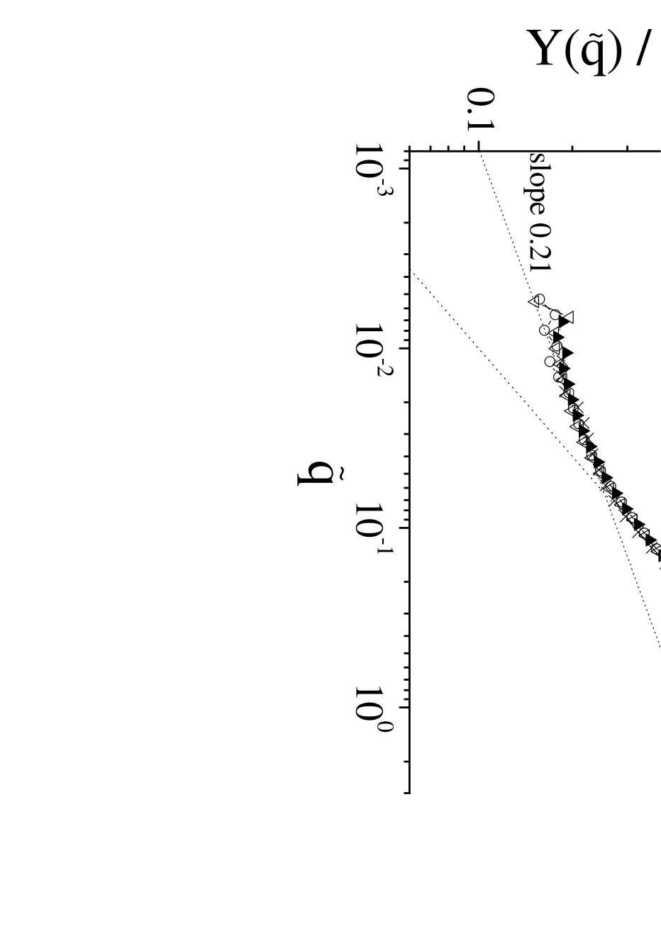
The scaling function exhibits the crossover from the power-law domain growth to the glassy dynamics. Looking Fig. 4 carefully, the scaling function is not universal, which is more apparent in lower temperature. Particularly the relaxation stops on the way at zero temperature. This indicates that the relaxation in the long time regime is thermally activated process. The system cannot escape from a metastable state without thermal assistance.
The scaling function represents the structure factor in the equilibrium state (). From the present scaling we obtain its shape even for the small wave numbers where is still far from equilibrium. While the growth law turned out to depend on the temperature , we find that is essentially independent of the temperature . This means that spatial correlation function in equilibrium has universal form independent of both and . The long wave length behavior of seems to obey a power law; . The roughness exponent is smaller than that in the Larkin regime and the value is consistent with the one for the random manifolds 55 5 The roughness exponent for the -dimensional system with -components deformation field is written as Nattermann and Scheidl 2000. The exponent corresponding to the present system has not known but expected to be between Huse et al. 1985 and Balents and Fisher 1993. Substituting these ’s and to the above formula instead of leads close values of and , respectively. . However it is more natural to expect that this agreement is a transient behavior that is approaching to zero because the present single harmonic model is considered to take single crossover to the Bragg glass regime Giamarchi and Doussal 1995; Giamarchi and Doussal World Scientific, Singapure, 1998.
V Summary and Discussions
In this paper the relaxation dynamics of the three dimensional elastic manifold in random potential has been studied. We especially focused on the crossover between the Larkin regime and the glassy regime, i.e., power-law domain growth and thermally activated relaxation. We proposed a new scaling method for the dynamical structure factor which encodes dynamical growth of the roughness of different origins and successfully applied it to explain the crossover between the Larkin and glassy regime. At a given temperature the structure factor out-of-equilibrium can be scaled by using the dynamical length and the Larkin length . Quite interestingly our analysis yields the structure factor in equilibrium, which is hard to observe in equilibrium simulations. The temperature dependence can be also taken care only by introducing a correction factor for the Larkin length. It turns out that the scaling function are universal and independent of the temperatures.
Although we analyzed the model with random potential that is periodic with respect to the deformation field, indication of QLRO was hardly observed. This will appear when the amplitude of phase fluctuation becomes greater than the period of the random potential, . The crossover region between the Larkin and Bragg glass regimes, however, persists for quite long time and has special importance in the dynamical aspect. This is because glassy behavior becomes serious at the early stage of the crossover. From the obtained scaling function , we can roughly estimate the end of the Larkin regimes as in Eq. (10) 66 6 From Fig. 4 we can read crossover wave number and then and . As a result where and corresponding to . . The growth rate of decreases quite quickly before reaches (see Fig. 2). (In fact almost all of in our simulations are smaller than and the system does not feel that the potential is periodic.) Therefore the early stage of the crossover, which has sufficiently long time range, hardly reflects the periodicity of the random potential and is similar to the crossover to the random manifold regime.
Acknowledgements.
The present work is supported by 21st Century COE program “Topological Science and Technology” and the Ministry of Education, Science, Sports and Culture, Grant-in-Aid for Young Scientists (A), 19740227, 2007. A part of the computation in this work has been done using the facilities of the Supercomputer Center, Institute for Solid State Physics, University of Tokyo.References
- Grüner (1988) G. Grüner, Rev. Mod. Phys. 60, 1129 (1988).
- Blatter et al. (1994) G. Blatter, M. V. Feigel’man, V. B. Geshkenbein, A. I. Larkin, and V. M. Vinokur, Rev. Mod. Phys. 66, 1125 (1994).
- Vincent et al. (Springer, Berlin, 1996) E. Vincent, J. Hammann, M. Ocio, J. P. Bouchaud, and L. F. Cgliandolo, in Proceedings of the Sitges Conference on Glassy Sytems ed. E. Rubi (Springer, Berlin, 1996).
- Nordblad and Svedlindh (World Scientific, Singapure, 1998) P. Nordblad and P. Svedlindh, Experiments on spin glasses in Spin Glasses and Random Fields ed. A. P. Young (World Scientific, Singapure, 1998).
- Bouchaud et al. (World Scientific, Singapure, 1998) J. P. Bouchaud, L. F. Cugliandolo, J. Kurchan, and M. Mezard, Out of equilibrium dynamics in spin-glasses and other glassy systems in Spin Glasses and Random Fields ed. A. P. Young (World Scientific, Singapure, 1998).
- Kawashima and Rieger (World Scientific, SIgapure, 2004) N. Kawashima and H. Rieger, Recent progress in spin glasses in Frustrated spin Systems ed. H. T. Diep (World Scientific, SIgapure, 2004).
- Debenedetti and Stillinger (2001) P. Debenedetti and F. H. Stillinger, Nature (London) 410, 259 (2001).
- Cugliandolo et al. (1996) L. F. Cugliandolo, J. Kurchan, and P. Le Doussal, Phys. Rev. Lett. 76, 2390 (1996).
- Yoshino (1996) H. Yoshino, J. Phys. A: Math. Gen. 29, 1421 (1996).
- Yoshino (1998) H. Yoshino, Phys. Rev. Lett. 81, 1493 (1998).
- Kolton et al. (2005) A. B. Kolton, A. Rosso, and T. Giamarchi, Phys. Rev. Lett. 95, 180604 (2005).
- Kolton et al. (2006) A. B. Kolton, A. Rosso, E. V. Albano, and T. Giamarchi, Phys. Rev. B 74, 140201(R) (2006).
- Bustingorry et al. (2006) S. Bustingorry, L. F. Cugliandolo, and D. Dominguez, Phys. Rev. Lett. 96, 027001 (2006).
- Bustingorry et al. (2007) S. Bustingorry, L. F. Cugliandolo, and D. Dominguez, Phy. Rev. B 75, 024506 (2007).
- Yoshino (unpublished) H. Yoshino (unpublished).
- Paul et al. (2004) R. Paul, S. Puri, and H. Rieger, Europhys. Lett. 68, 881 (2004).
- Rieger et al. (2005) H. Rieger, G. Schehr, and R. Paul, Prog. Theo. Phys. Suppl. 157, 111 (2005).
- Kisker et al. (1996) J. Kisker, L. Santen, M. Schreckenberg, and H. Rieger, Phys. Rev. B 53, 6418 (1996).
- Komori et al. (1999) T. Komori, H. Yoshino, and H. Takayama, J. Phys. Soc. Jpn 68, 3387 (1999).
- Huse et al. (1985) D. A. Huse, C. L. Henley, and D. S. Fisher, Phys. Rev. Lett. 55, 2924 (1985).
- Villain (1984) J. Villain, Phys. Rev. Lett. 52, 1543 (1984).
- Huse and Fisher (1987) D. A. Huse and D. S. Fisher, Phys. Rev. B. 35, 6841 (1987).
- Fisher and Huse (1991) D. S. Fisher and D. A. Huse, Phys. Rev. B 43, 10728 (1991).
- Mikheev et al. (1995) L. V. Mikheev, B. Drossel, and M. Kardar, Phys. Rev. Lett. 75, 1170 (1995).
- Fukuyama and Lee (1978) H. Fukuyama and P. A. Lee, Phys. Rev. B 17, 535 (1978).
- Lee and Rice (1979) P. A. Lee and T. M. Rice, Phys. Rev. B 19, 3970 (1979).
- Giamarchi and Doussal (1995) T. Giamarchi and P. Le Doussal, Phys. Rev. B 52, 1242 (1995).
- Larkin (1970) A. I. Larkin, Sov. Phys. JETP 31, 784 (1970).
- Imry and Ma (1975) Y. Imry and S. Ma, Phys. Rev. Lett. 21, 1399 (1975).
- Fisher (1985) D. S. Fisher, Phys. Rev. B 31, 7233 (1985).
- Fisher (1986) D. S. Fisher, Phys. Rev. Lett. 56, 1964 (1986).
- Feigel’man et al. (1989) M. V. Feigel’man, V. B. Geshkenbein, A. I. Larkin, and V. M. Vinokur, Phys. Rev. Lett. 63, 2303 (1989).
- Bouchaud et al. (1991) J. P. Bouchaud, M. Mézard, and J. S. Yedidia, Phys. Rev. Lett. 67, 3840 (1991).
- Nattermann (1990) T. Nattermann, Phys. Rev. Lett 64, 2454 (1990).
- Korshunov (1993) S. E. Korshunov, Phys. Rev. B 48, 3969 (1993).
- Giamarchi and Doussal (World Scientific, Singapure, 1998) T. Giamarchi and P. Le Doussal, Statics and Dynamics of Disordered Elastic Systems in Spin Glasses and Random Fields ed. A. P. Young (World Scientific, Singapure, 1998).
- Lindemann (1910) F. Lindemann, Z. Phys. 11, 609 (1910).
- Honeycutt (92) R. L. Honeycutt, Phys. Rev. A 45, 600 (92).
- Schehr and Doussal (2005) G. Schehr and P. Le Doussal, Europhys. Lett. 77, 290 (2005).
- Nattermann and Scheidl (2000) T. Nattermann and S. Scheidl, Adv. Phys. 49, 607 (2000).
- Balents and Fisher (1993) L. Balents and D. S. Fisher, Phys. Rev. B 48, 5949 (1993).