Modeling Phase-resolved Observations of the Surfaces of Magnetic Neutron Stars
Abstract
Recent observations by XMM-Newton detected rotational pulsations in the total brightness and spectrum of several neutron stars. To properly interpret the data, accurate modeling of neutron star emission is necessary. Detailed analysis of the shape and strength of the rotational variations allows a measurement of the surface composition and magnetic field, as well as constrains the nuclear equation of state. We discuss our models of the spectra and light curves of two of the most observed neutron stars, RX J1856.53754 and 1E 1207.45209, and discuss some implications of our results and the direction of future work.
Keywords:
stars: atmospheres - stars: magnetic fields - stars: neutron - stars: rotation - X-rays: starsClassification:
97.60.Jd; 26.60.Kp; 95.30.Gv; 95.75.-z; 95.85.Nv; 97.10.-q1 Introduction
Thermal radiation from the surface of neutron stars (NSs) can provide invaluable information on the physical properties and evolution of NSs. NS properties, such as the mass and radius , in turn depend on the poorly constrained physics of the stellar interior, such as the nuclear equation of state (EOS) and quark and superfluid/superconducting properties at supra-nuclear densities. Many NSs are also known to possess strong magnetic fields ( G), with some well above the quantum critical value ( G).
The observed thermal radiation originates in a thin atmospheric layer (with scale height cm) that covers the stellar surface. To properly interpret the observations of NS surface emission and to provide accurate constraints on their physical properties, it is important to understand in detail the radiative behavior of NS atmospheres in the presence of strong magnetic fields (see (pavlovetal95; holai01; zavlinpavlov02; holai03; zavlin07), for more detailed references on observations and on previous works in NS atmosphere modeling). The properties of the atmosphere, such as the chemical composition, EOS, and radiative opacities, directly determine the characteristics of the observed spectrum. While the surface composition of the NS is unknown, a great simplification arises due to the efficient gravitational separation of light and heavy elements (alcockillarionov80). A pure hydrogen atmosphere is expected even if a small amount of accretion/fallback occurs after NS formation; the total mass of hydrogen needed to form an optically thick atmosphere can be less than g. On the other hand, a heavy element atmosphere may be possible if no accretion takes place.
The strong magnetic fields present in NS atmospheres significantly increase the binding energies of atoms, molecules, and other bound states (see (lai01), for a review). Abundances of these bound states can be appreciable in the atmospheres of cold NSs (i.e., those with surface temperature K; (laisalpeter97; potekhinetal99)). In addition, the presence of a magnetic field causes emission to be anisotropic and polarized; this must be taken into account when developing radiative transfer codes. The most comprehensive early studies of magnetic NS atmospheres focused on a fully ionized hydrogen plasma and moderate field strengths ( G; (miller92; shibanovetal92; pavlovetal94; zaneetal00)). These models are expected to be valid only for relatively high temperatures. More recently, atmosphere models in the ultra-strong field ( G) and relevant temperature regimes have been presented ((ozel01; zaneetal01; holai03; lloyd03; vanadelsberglai06); see also (bezchastnovetal96; bulikmiller97), for early work), and all of these rely on the assumption of a fully ionized hydrogen composition. Magnetized non-hydrogen atmospheres have been studied by (miller92; rajagopaletal97), but because of the complexity of the atomic physics, the models were necessarily crude (see (moriho07), for more details). Only recently has self-consistent atmosphere models (hoetal03; potekhinetal04; moriho07) using the latest EOS and opacities for partially ionized hydrogen (potekhinchabrier03; potekhinchabrier04) and mid- elements (morihailey02; morihailey06) been constructed.
The atmosphere models discussed above only describe emission from a local patch of the stellar surface. By taking into account surface magnetic field and temperature distributions, we can construct more physically correct models of emission from NSs. However, these spectra from the whole NS surface are necessarily model-dependent, as the and distributions are unknown. Nevertheless, detailed comparisons of the models with rotation phase-resolved observations is a powerful tool to study NSs, e.g., spectral features that vary with phase are essential to disentangling magnetic field effects from other parameters and to probe the magnetic field geometry on the surface of the star. Indeed there have been recent works attempting to fit magnetic atmosphere spectra to observations of NSs (see (ho07), and references therein). Here we describe some of the details and observational applications of our work.
2 Model for Neutron Star Surface Emission
In order to construct models of emission from the entire NS surface, we first build atmosphere models for a given effective temperature and magnetic field strength and direction relative to the surface normal; these (local) models describe a patch of the NS surface. In the presence of magnetic fields G, radiation propagates in two photon polarization modes (see, e.g., (meszaros92)); therefore, the atmosphere models are obtained by solving the radiative transfer equations for the two coupled polarization modes (see (holai01; hoetal03; hoetal07; potekhinetal04), for details on the construction of the atmosphere models). In addition to and , the atmosphere models have a dependence, through hydrostatic balance, on the surface gravity , where the gravitational redshift is given by ; however, the resulting spectra do not vary significantly using different values of around cm s-2 (pavlovetal95).
Next, the entire NS surface is divided into regions with different and . Relatively simple surface distributions of and are adopted: we assume the surface is symmetric (in and ) about the magnetic equator and divide the hemisphere into several magnetic colatitudinal regions. An example parametrization is given in Table 1; note that the magnetic field distribution is roughly dipolar. Emission from any point within a colatitudinal region is given by the atmosphere model for that region.
| magnetic colatitude | |||
|---|---|---|---|
| (deg) | ( G) | (deg) | ( K) |
| 020 | 6 | 0 | 7 |
| 2050 | 5 | 30 | 6 |
| 5070 | 4 | 60 | 5 |
| 7090 | 3 | 90 | 4 |
Finally, the spectra from the entire NS surface is computed by summing over the emission from the different regions for a given rotation phase (see (pavlovzavlin00; ho07), for details). The observed emission depends on two angles (): is the angle between the rotation and magnetic axes and is the angle between the rotation axis and the direction to the observer. We also account for the bending of the path of light due to gravity, which causes more of the NS surface to be visible ( and as compared to without light-bending for and km and 14 km, respectively; see (pechenicketal83; beloborodov02)).
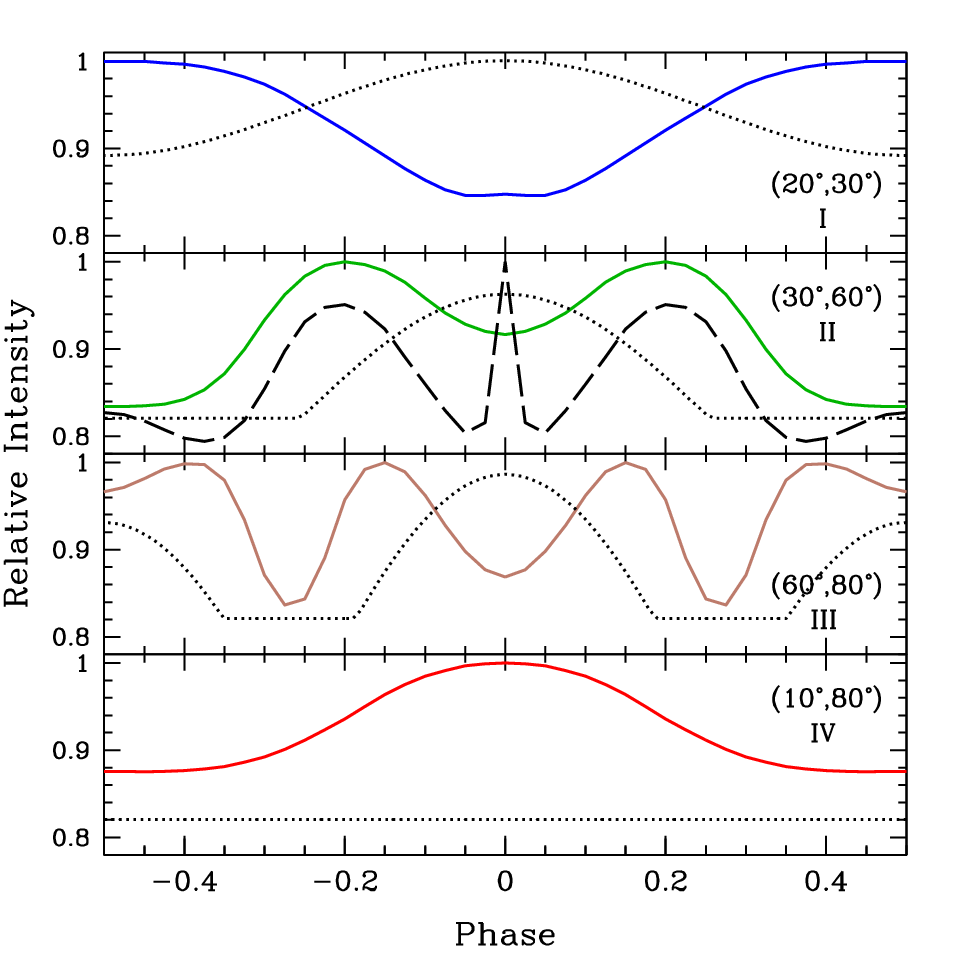
Figure 1 shows the light curves, for various geometries (), of the NS model using the parametrization given in Table 1, , and cm s-2. We also plot the analytic light curves from (beloborodov02) for isotropic emission from two antipodal hot spots (see (zavlinpavlov98; bogdanovetal07), for examples of pulse profiles from non-magnetic hydrogen atmosphere hot spots). The classification scheme (for isotropically-emitting hot caps) is defined in (beloborodov02): (I) only the primary cap is visible, and the pulse profile is purely sinusoidal with a single peak, (II) the opposite cap is seen around pulse minimum due to relativistic light-bending, which reduces the strength of the modulation, (III) the primary cap is not seen during a segment of the rotation, and (IV) both spots are seen at all phases and thus there is no modulation.
Several important features are evident from a comparison of magnetic atmosphere emission to that of isotropic emission. The angular-dependence of the radiation (or beam pattern) manifests as a narrow “pencil-beam” along the direction of the magnetic field and a broad “fan-beam” at intermediate angles (see (pavlovetal94; lloyd03), for beam patterns and spectra at various ). As discussed in (pavlovetal94), the pencil-beam is the result of the lower opacity at angles , where keV is the electron cyclotron energy; the width of the pencil-beam is thus , and the radiation is more strongly beamed at higher magnetic fields. This narrow beam is seen in the (50∘,50∘)-light curve plotted in Figure 1, which is the only instance shown that has the observer’s line-of-sight exactly crossing the magnetic cap and coinciding with the peak of the isotropic emission. Also evident is the fan-beam (most obvious in the light curves of classes II and III), which occur on either side of the magnetic cap and can increase the number of light-curve peaks. Finally, the anisotropic beam pattern (combined with the surface temperature variation) can produce an apparent phase shift compared to isotropic emission and modulation when an isotropic beam pattern suggests none (c.f. class IV).
3 RX J1856.53754
RX J1856.53754 is one of the brightest, nearby isolated NSs (kaplanvankerkwijk07), and considerable observational resources have been devoted to its study. Recently, XMM-Newton observations uncovered pulsations from RX J1856.53754 with a period of 7 s and an upper limit on the period derivative (tiengomereghetti07; mereghettitiengo07). The EPIC-pn and MOS light curves are shown in Figure 2. Several characteristics of the observed light curves suggest possible values of and : (1) the 1.6%0.2% amplitude of the pulsations, (2) a single peak (or two peaks close in phase, as may be the case for the pn light curve) per rotation, and (3) no significant energy-dependence for the single observation and small energy-dependence for all XMM-Newton data (ho07; tiengomereghetti07).

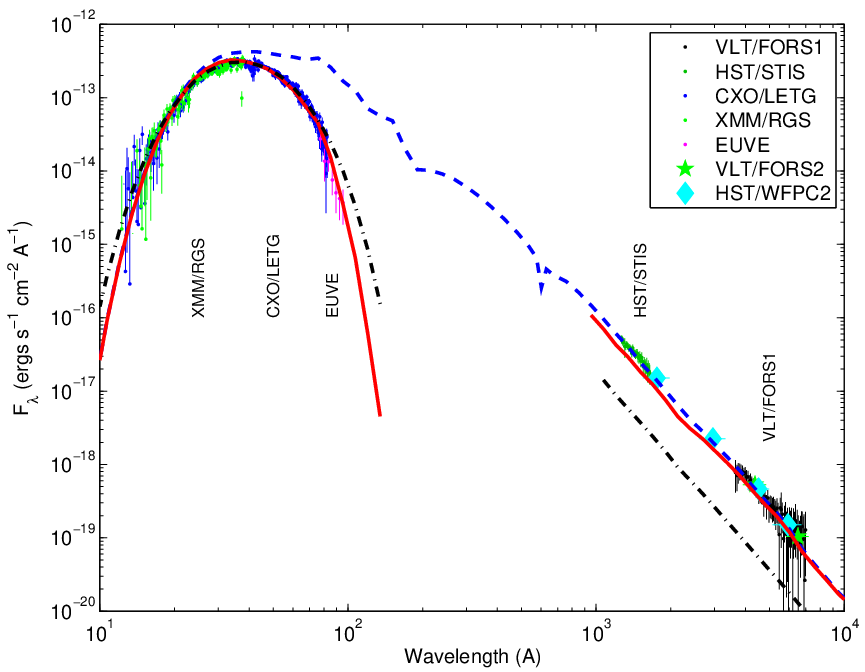
In previous work (hoetal07), we found that our models of a magnetic, partially ionized hydrogen atmosphere matches well the entire spectrum, from X-rays to optical, of RX J1856.53754 [best-fit parameters: gravitational redshift , magnetic field G, and radius km, where ; see Figure 3]. With the discovery of rotational modulation of the X-ray emission (tiengomereghetti07), we use the light curves predicted by our model (described in the previous section) to constrain the geometry () of RX J1856.53754 (ho07). We find angles of and (example fits ares shown in Figure 2). This indicates that either the rotation and magnetic axes are closely aligned or we are essentially seeing down the spin axis of the NS (see also (brajeromani02)).
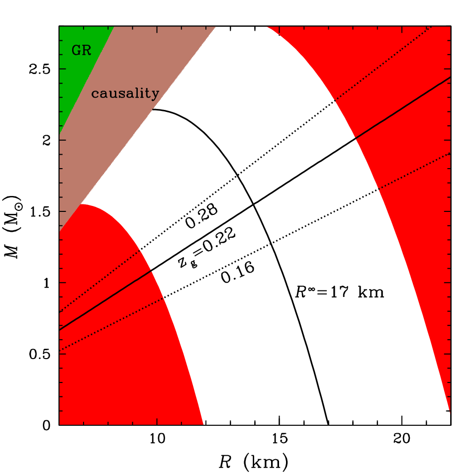
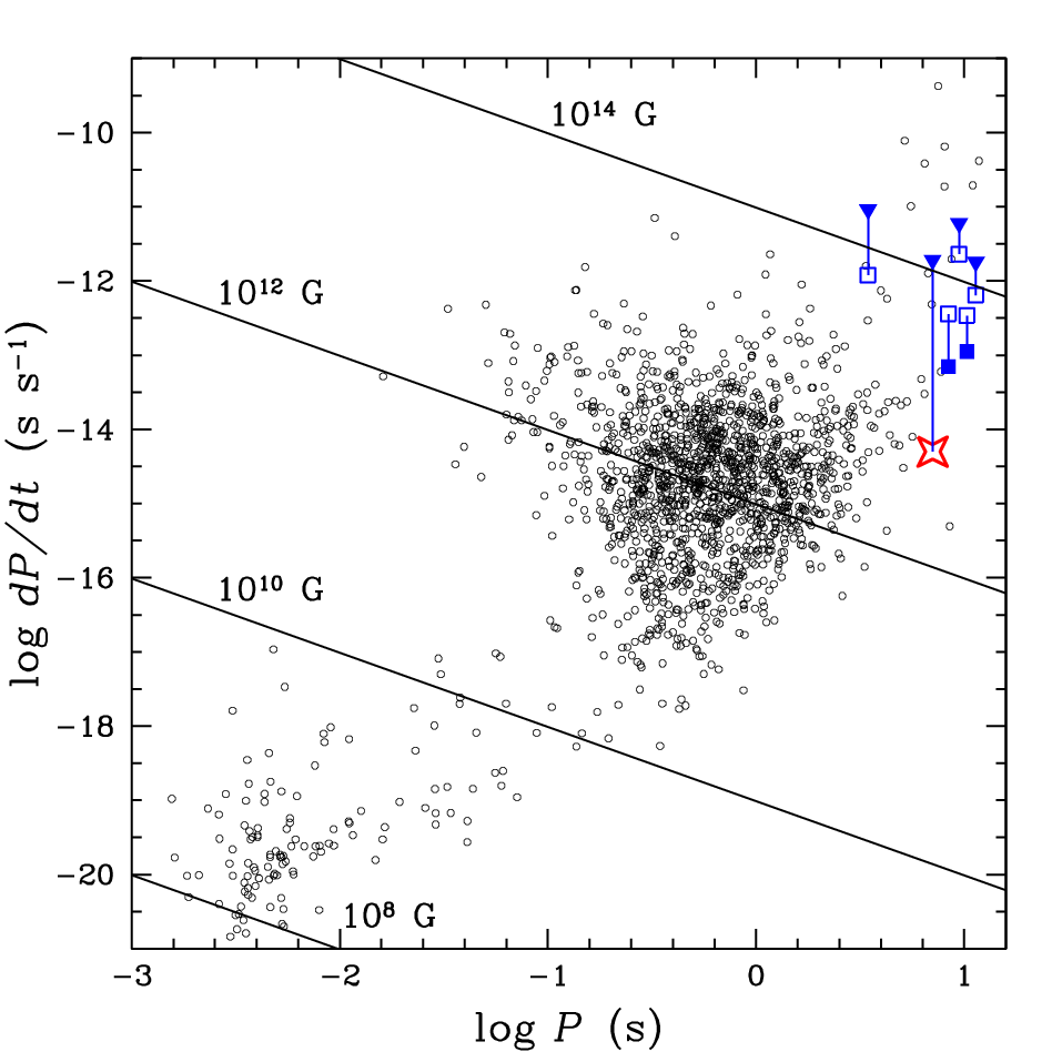
From the results of our modeling of the phase-resolved observations, we can better determine where RX J1856.53754 belongs in the broader context of NS studies. For example, Figure 4 shows the constraints placed on the mass-radius relationship for NSs. Our results imply a relatively stiff but standard nuclear EOS (see, e.g., (lattimerprakash07)). Also if RX J1856.53754 is losing rotational energy by magnetic dipole radiation, the rate of spindown is given by ; this is well below the upper limit obtained by (tiengomereghetti07) and illustrated in Figure 5. Note that RX J1856.53754 has not been detected in the radio (brazierjohnston99; burgayetal07; kondratievetal07), though its location in space (see Figure 5) is below the theoretical death line for radio pulsars.
4 1E 1207.45209
1E 1207.45209 is a NS (with spin period = 0.424 s) in the center of supernova remnant G 296.5+10.0. Its X-ray spectrum is remarkable in that it shows two broad absorption features at and keV (mereghettietal02; sanwaletal02; morietal05; delucaetal07; gotthelfhalpern07b). Even more surprising is that these features show greater phase-variability than the continuum spectrum (bignamietal03; delucaetal04). Proposed models involving ion cyclotron or atomic lines from a light element atmosphere at G (sanwaletal02; turbinerlopez04) seem unlikely due to weakening of line strengths by vacuum resonance effects (holai03; holai04; vanadelsberglai06) or low abundance of the ionization states possibly responsible for the observed lines (morihailey06). Recent timing analysis also imply G (by assuming vacuum dipole braking); this suggests the spectral features are electron cyclotron lines (gotthelfhalpern07). Alternatively, (haileymori02; morihailey06) proposed a mid- element atmosphere at G. We are studying this last case by building atmosphere models composed of mid- elements (see (moriho07), for details) in an attempt to fit the phase-resolved observations.
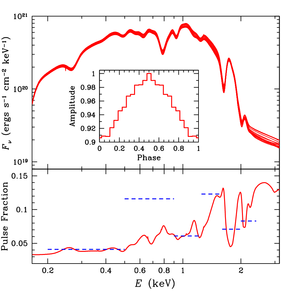
As an illustration of our models, Figure 6 shows the phase-resolved model oxygen atmosphere spectra, light curve, and pulse fraction [, where is the count spectrum]. We assume here that , , and the NS surface is parametrized by K and []= () for magnetic colatitudes 0–5∘ and () for colatitudes 6–20∘. Note that our models roughly match the continuum shape and line locations and strengths of the phase-averaged spectrum of 1E 1207.45209. More detailed analysis will be reported elsewhere.
In summary, we discussed briefly our continuing work on understanding the emission process of NS surfaces, as well as detailed comparisons of our models to phase-resolved observations of the NSs RX J1856.53754 and 1E 1207.45209. Analyses of other sources is ongoing. In the near future, we are integrating our model spectra into XSPEC for community use (hoetal07b).
References
- (1) G. G. Pavlov, Yu. A. Shibanov, V. E. Zavlin, and R. D. Meyer, “Neutron Star Atmospheres” in Lives of the Neutron Stars, edited by M. A. Alpar, Ü. Kiziloğlu, and J. van Paradijs, Kluwer, Boston, 1995, pp.71–90.
- (2) W. C. G. Ho and D. Lai, MNRAS 327, 1081–1096 (2001).
- (3) V. E. Zavlin and G. G. Pavlov, “Modeling Neutron Star Atmospheres” in Proc. 270 Heraeus Seminar on Neutron Stars, Pulsars and Supernova Remnants, edited by W. Becker, H. Lesch, and J. Trümper, MPE Rep. 278, MPE, Garching, 2002, pp.263–272.
- (4) W. C. G. Ho and D. Lai, MNRAS 338, 233–252 (2003).
- (5) V. E. Zavlin, “Thermal Emission from Isolated Neutron Stars: Theoretical and Observational Aspects” in 363rd Heraeus Seminar on Neutron Stars and Pulsars, submitted, astro-ph/0702426 (2007).
- (6) C. Alcock and A. Illarionov, ApJ 235, 534–553 (1980).
- (7) D. Lai, Rev. Mod. Phys. 73, 629–662 (2001).
- (8) D. Lai and E. E. Salpeter, ApJ 491, 270–285 (1997).
- (9) A. Y. Potekhin, G. Chabrier, and Yu. A. Shibanov, Phys. Rev. E 60, 2193–2208 (1999).
- (10) M. C. Miller, MNRAS 255, 129–145 (1992).
- (11) Yu. A. Shibanov, V. E. Zavlin, G. G. Pavlov, and J. Ventura, A&A 266, 313–320 (1992).
- (12) G. G. Pavlov, Yu. A. Shibanov, J. Ventura, and V. E. Zavlin, A&A 289, 837–845 (1994).
- (13) S. Zane, R. Turolla, and A. Treves, ApJ 537, 387–395 (2000).
- (14) F. Özel, ApJ 563, 276–288 (2001).
- (15) S. Zane, R. Turolla, L. Stella, and A. Treves, ApJ 560, 384–389 (2001).
- (16) D. A. Lloyd, MNRAS, submitted, astro-ph/0303561 (2003).
- (17) M. van Adelsberg and D. Lai, MNRAS 373, 1495–1522 (2006).
- (18) V. G. Bezchastnov, G. G. Pavlov, Yu. A. Shibanov, and V. E. Zavlin, “Radiative Opacities and Photosphere Models for Soft Gamma Repeaters” in AIP Conf. Proc. 384, Gamma-Ray Bursts, edited by C. Kouveliotou, M. F. Briggs, and G. J. Fishman, AIP, Woodbury, 1996, pp.907–911.
- (19) T. Bulik and M. C. Miller, MNRAS 288, 596–608 (1997).
- (20) M. Rajagopal, R. W. Romani, and M. C. Miller, ApJ 479, 347–356 (1997).
- (21) K. Mori and W. C. G. Ho, MNRAS 377, 905–919 (2007).
- (22) W. C. G. Ho, D. Lai, A. Y. Potekhin, and G. Chabrier, ApJ 599, 1293–1301 (2003).
- (23) A. Y. Potekhin, D. Lai, G. Chabrier, and W. C. G. Ho, ApJ 612, 1034–1043 (2004).
- (24) A. Y. Potekhin and G. Chabrier, ApJ 585, 955–974 (2003).
- (25) A. Y. Potekhin and G. Chabrier, ApJ 600, 317–323 (2004).
- (26) K. Mori and C. J. Hailey, ApJ, 564, 914–929 (2002).
- (27) K. Mori and C. J. Hailey, ApJ, 648, 1139–1155 (2006).
- (28) W. C. G. Ho, MNRAS 380, 71–77 (2007).
- (29) P. Mészáros, High-Energy Radiation from Magnetized Neutron Stars, University of Chicago Press, Chicago, 1992.
- (30) W. C. G. Ho, D. L. Kaplan, P. Chang, M. van Adelsberg, and A. Y. Potekhin, MNRAS 375, 821–830 (2007).
- (31) G. G. Pavlov and V. E. Zavlin, ApJ 529, 1011–1018 (2000).
- (32) K. R. Pechenick, C. Ftaclas, and J. M. Cohen, ApJ 274, 846–857 (1983).
- (33) A. M. Beloborodov, ApJL 566, L85–88 (2002).
- (34) V. E. Zavlin and G. G. Pavlov, A&A 329, 583–598 (1998).
- (35) S. Bogdanov, G. B. Rybicki, and J. E. Grindlay, ApJ, in press, astro-ph/0612791 (2007).
- (36) D. L. Kaplan and M. H. van Kerkwijk, this proceedings.
- (37) A. Tiengo and S. Mereghetti, ApJL 657, L101–104 (2007).
- (38) S. Mereghetti and A. Tiengo, this proceedings.
- (39) T. M. Braje and R. W. Romani, ApJ, 580, 1043–1047 (2002).
- (40) J. M. Lattimer and M. Prakash, Phys. Rep. 442, 109–165 (2007).
- (41) R. N. Manchester, G. B. Hobbs, A. Teoh, and M. Hobbs, AJ 129, 1993–2006 (2005).
- (42) F. Haberl, Ap&SS 308, 181–190 (2007).
- (43) K. T. S. Brazier and S. Johnston, MNRAS 305, 671–679 (1999).
- (44) M. Burgay, this proceedings.
- (45) V. I. Kondratiev, this proceedings.
- (46) S. Mereghetti, A. De Luca, P. A. Caraveo, W. Becker, R. Mignani, and G. F. Bignami, ApJ 581, 1280–1285 (2002).
- (47) D. Sanwal, G. G. Pavlov, V. E. Zavlin, and M. A. Teter, ApJL 574, L61–L64 (2002).
- (48) K. Mori, J. C. Chonko, and C. J. Hailey, ApJ, 631, 1082–1093 (2005).
- (49) A. De Luca, this proceedings.
- (50) E. V. Gotthelf and J. P. Halpern, this proceedings.
- (51) G. F. Bignami, P. A. Caraveo, A. De Luca, and S. Mereghetti, Nature 423, 725–727 (2003).
- (52) A. De Luca, S. Mereghetti, P. A. Caraveo, M. Moroni, R. P. Mignani, and G. F. Bignami, A&A 418, 625–637 (2004).
- (53) A. V. Turbiner and J. C. López Vieyra, Mod. Phys. Lett. A 19, 1919–1923 (2004).
- (54) W. C. G. Ho and D. Lai, ApJ 607, 420–425 (2004).
- (55) E. V. Gotthelf and J. P. Halpern, ApJL 664, L35–L38 (2007).
- (56) C. J. Hailey and K. Mori, ApJL, 578, L133–L136 (2002).
- (57) W. C. G. Ho, A. Y. Potekhin, G. Chabrier, et al., in preparation.