Influence of the isospin and hypercharge chemical potentials on the location of the CEP in the $\mu_{B}-T$ phase diagram of the $SU(3)_{L}\times SU(3)_{R}$ chiral quark model

One has some freedom in choosing the set of equations which determines the 13 parameters of the model, namely $m_{0}^{2},f_{1},f_{2},g,g_{F},$ $v_{0},v_{3},v_{8},$ $\epsilon_{0},\epsilon_{3},\epsilon_{8}$ and $l_{f},l_{b}$. These latter two parameters are the fermionic and bosonic renormalization scales. For the parametrization we follow the method described in kovacs07 where the renormalization of the model was also discussed. The only difference in the present case is the appearance of $v_{3}$ and $\epsilon_{3}$. Since at zero temperature and densities the effect of isospin breaking is small we use the same values for $l_{f}$ and $l_{b}$ as in kovacs07 where these were determined by minimizing the deviation of the predicted mass spectrum from the physical one. The external fields are determined from the equations of state (12), (13), (14) once the remaining 8 parameters are known.

In order to avoid the appearance of negative propagator mass squares in the one-loop finite temperature calculations in the broken symmetry phase we use the Optimized Perturbation Theory (OPT) of Ref. hatsuda98. This amounts to replace the mass parameter $-m_{0}^{2}$ in the Lagrangian with an effective, eventually temperature-dependent, mass parameter $m^{2}$:

The counterterm $\Delta m^{2}$ is taken into account first at one-loop level, while $m^{2}$ will replace $m_{0}^{2}$ in all the tree-level masses and is determined using the criterion of fastest apparent convergence (FAC). We have chosen to implement this criterion by requiring that for $\pi^{+}$ the one-loop mass calculated at vanishing external momentum stays equal to the tree-level mass ($M_{\pi^{+}}=m_{\pi^{+}}$). We have checked that imposing this equation for the neutral pion rather than the charged one results in no significant changes in the parameters. We note here that we were forced to use the definition $M_{\pi^{+}}^{2}=-iG^{-1}(p=0)$ instead of defining the one-loop mass as the pole of the propagator because in this latter case the solution to the gap equation, to be presented below, ceases to exist above a certain temperature, in accordance with previous investigations using the OPT hatsuda98; herpay06.

As described in details in kovacs07, with the application of FAC one can eliminate the effective mass parameter $m^{2}$ in favor of the tree-level pion mass $m_{\pi^{+}}^{2}$ in all the other tree-level masses of the propagators used to calculate the one-loop self-energies:

In this way one obtains the following gap equation

where $\Sigma_{\pi^{+}}$ denotes the self-energy of $\pi^{+}$ shown diagrammatically in Fig. 1. Equation (18) is the first from a set of four coupled non-linear equations which determines $m_{0}^{2},f_{1},f_{2},g$, if one knows $g_{F},v_{0},v_{3},v_{8}$. Two further equations of the set are given by the one-loop equation for the $\eta$ and $K^{+}$ pole masses

where ${\mathcal{M}}^{2}_{\textrm{tree}}$ is the tree-level mass squared matrix of the mixing sector without the mass parameter $m^{2}$, the orthogonal matrix $\tilde{O}_{P}$ diagonalizes the expression in the round bracket, and $\Sigma_{0,3,8}$ is the self-energy matrix of the pseudoscalar mixing sector. This matrix is determined numerically. The last equation in the set is the FAC criterion for the kaon, which requires $\textnormal{Re}\Sigma_{K^{+}}(p^{2}=M_{K^{+}}^{2})-\Delta m^{2}=0$.

The parameters $g_{F},v_{0},v_{3},v_{8}$ are determined as follows. A linear combination of $v_{0}$ and $v_{8}$ is determined by the tree-level PCAC relation for the pion decay constant (see Appendix of Lenaghan00)

One can see from (11) that the same linear combination enters the expression of the average mass of the two light constituent quarks, so that the Yukawa coupling is given by $g_{F}=(M_{u}+M_{d})/f_{\pi}$. Another linear combination of $v_{0}$ and $v_{8}$ appears in the expression of $M_{s}$ in (11) which together with the PCAC relation (21) determines $v_{0}$ and $v_{8}$:

The remaining parameter, $v_{3}$ is obtained by requiring that the difference between the tree-level masses of $\pi^{+}$ and $\pi^{0}$ equals the physical value ($\Delta m_{\pi}$):

This equation has two roots for $v_{3}$, a negative and a positive one. The positive root would give $m_{K^{0}}<m_{K^{+}}$ for the kaon masses. Since the opposite relation holds in nature, we choose the negative solution which is the physically valid one.

We use the following values for the physical quantities: $m_{\pi^{+}}=139.57$ MeV, $\Delta m_{\pi}=4.594$ MeV, $M_{K^{+}}=493.677$ MeV, $M_{\eta}=547.8$ MeV, $f_{\pi}=93$ MeV, $(M_{u}+M_{d})/2=313$ MeV, $M_{s}=530$ MeV and in addition $l_{b}=520$ MeV and $l_{f}=1210$ MeV for the two renormalization scales.

The introduction of the chemical potential for a system with a set of conserved charge operators is reviewed below. For vanishing external fields the Lagrangian (1) is invariant under the following global vector transformations

where $G$ denotes the representation of the baryon (B), third component of the isospin (I) and hypercharge (Y) operators which are related to the diagonal generators as $B=\sqrt{\frac{3}{2}}\lambda_{0}$, $I=\frac{1}{2}\lambda_{3}$ and $Y=\frac{1}{\sqrt{3}}\lambda_{8}$. The coefficients in front of the diagonal matrices are chosen such as to obtain the right quantum numbers when applying the operators on the quark fields. The consequence of this symmetry is the existence of conserved Noether vector-currents

The conserved charge is defined as $Q^{G}=\int d^{3}xJ_{0}^{G}(x)$. In terms of particle number operators the conserved baryon, isospin and hypercharges read as

Note the different sign of $N_{K^{0}},N_{\bar{K}^{0}},N_{\kappa^{0}},N_{\bar{\kappa}^{0}}$ in $Q^{I}$ relative to $Q^{Y}$. This is because the particles $K^{0},\bar{K}^{0},\kappa^{0},\bar{\kappa}^{0}$ fall into different doublets from the point of view of the $I_{3}$ and $Y$ quantum numbers: $K^{0},K^{+}$ and $K^{-},\bar{K}^{0}$ form a $I_{3}$ doublet while $K^{0},K^{-}$ and $K^{+},\bar{K}^{0}$ form a $Y$ doublet (likewise for scalars).

The statistical density matrix of the system is given by

with $G$ going over $B,I,Y$ in the summation over this index. Using (26), (27), (28) one can rewrite (29) by regrouping the terms in the exponent according to different number operators and obtain $\rho=\exp[-\beta(H-\mu_{i}N_{i})],$ where $i$ goes over all the non-singlet particles to which the following chemical potentials were introduced in terms of $\mu_{B},\mu_{I},\mu_{Y}$:

The singlet particles ($\pi^{0},$ $\eta,$ $\eta^{\prime},$ $a_{0}^{0},$ $\sigma,$ and $f_{0}$) do not contribute to the conserved charges and in consequence no chemical potential is introduced for them. By looking at (30) one can see that different members of a given multiplet (e.g. $\pi^{+}$ and $\pi^{-}$) acquire a different combination of the baryon, isospin and hypercharge chemical potentials, which means that the chemical potentials remove completely the degeneracy between the members of the multiplets which we observe in the vacuum, both at tree and one-loop level. We have to keep track of the effect of 21 individually different particles, which makes things more complicated than in previous studies of this model.

The effect of the chemical potentials is taken into account through the propagators which are introduced using the definition familiar from the theory of many-body systems. The relativistic formalism was developed in zimmerman72 and is reviewed in Appendix A, where the calculation of the self-energy using the finite-density Green’s function is also sketched.

In order to see explicitly that the particle and its antiparticle reflect differently the presence of a finite density medium we give here the tree-level propagators of $K^{+}$ and $K^{-}$:

where $\displaystyle n_{K^{\pm}}(E_{\bf p})=\frac{1}{e^{\beta(E_{\bf p}-\mu_{K^{\pm}})}-1}$ and $E_{\bf p}=\sqrt{{\bf p}^{2}+m_{K^{\pm}}^{2}}$. The interpretation of the terms on the right hand side of (31) is as follows (from left to right): addition of a particle, removal of a particle, addition of an antiparticle, removal of an antiparticle. Note, that in the propagator of the $K^{+}$ the particle is $K^{+}$ and the antiparticle is $K^{-}$, while in the propagator of the $K^{-}$ the particle is $K^{-}$ and the antiparticle is $K^{+}$.

For all the other scalar and pseudoscalar fields the propagators can be written analogously using the chemical potentials defined in (30). For the fermions the propagators are given in Appendix A.

With the parameters fixed in the previous section, we can solve the model at finite temperature and density using the formalism described in Section II.2 and in Appendix A. One calculates the 1-loop integrals entering the finite temperature and density version of the equations which determine the state of the system: the three equations of state (12), (13), (14) and the gap-equation for $m_{\pi^{+}}$ (18). The relevant integrals are given in Appendix A. An observed smooth variation of the order parameters with the intensive parameter ($T$, or $\mu_{B,I,Y}$) indicates analytic crossover type transition. A first order phase transition is signaled by the multivaluedness of either one of the three condensates in a given range of variation of the intensive parameter. The point where by varying some parameter(s) the nature of the phase transition changes from crossover to first order one corresponds to a second order phase transition.

The critical end point (CEP) is a second order phase transition point on the $\mu_{B}-T$ plane where by increasing $\mu_{B}$ the phase transition as a function of $T$ changes from crossover to first order ($\mu_{I}$ and $\mu_{Y}$ are kept constant). At vanishing $\mu_{I}$ and $\mu_{Y}$ the CEP is located in the point $(T,\mu_{B})_{\textnormal{CEP}}=(63.08,960.8)$ MeV. The pseudo-critical temperature at vanishing chemical potentials is $T_{c}(\mu_{B,I,Y}=0)=157.98$ MeV.

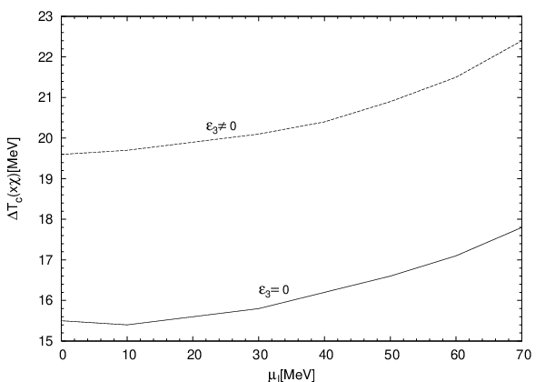
Here it is important to note that, with the explicit isospin breaking taken into account, these values have significantly changed with respect to those obtained without isospin breaking at all (neither explicit nor spontaneous): $(T,\mu_{B})_{\textnormal{CEP}}=(74.83,895.38)$ MeV and $T_{c}(\mu_{B,I,Y}=0)=154.84$ MeV kovacs07. At first sight this is surprising since we have seen that at $T=\mu=0$ the effect of the explicit symmetry breaking is minimal. The difference is due to the behavior of the $v_{3}$ with the temperature. Without explicit isospin symmetry breaking $v_{3}$ is identically zero for $\mu_{I}=0$. When $\epsilon_{3}\neq 0$ one can see by looking at the reference curve of Fig. 2 that with increasing temperature $v_{3}$ is decreasing significantly compared to its $T=0$ value and reaches a minimum around the phase transition point where the influence of $v_{3}$ becomes the strongest. The l.h.s. panel of Fig. 2 shows that the baryochemical potential magnifies this effect, implying that approaching the CEP the influence of $v_{3}$ is even stronger. According to our conjecture made in kovacs07 that a smoother crossover at $\mu_{B}=0$ will require a larger value of $\mu_{B}$ to turn the phase-transition in $T$ into a first order one, implying a larger value of $\mu_{B,\textnormal{CEP}}$, we can expect that the larger value of $\mu_{B,\textnormal{CEP}}$ in the case of the explicit isospin breaking compared to the case in which the isospin breaking is absent corresponds to a higher value of the width of the chiral susceptibility $\Delta T_{c}(x\chi)$. Indeed, by looking at Fig. 3 one can see, that in the case with explicit isospin symmetry breaking $\Delta T_{c}(x\chi)$ increased by $\sim 20\%$, approaching the value of $\Delta T_{c}(\chi_{\bar{\psi}\psi})=28(5)(1)$ MeV at at $\mu_{I}=0$. This value was obtained on the lattice in Ref. fk06 after the extrapolation in the continuum limit was done, though in this lattice investigation the effect of isospin breaking was not taken into account. It would be interesting to see whether similar effect is produced on lattice when $m_{u}\neq m_{d}$.

Varying $\mu_{I}$ and $\mu_{Y}$ the location of the CEP in the $\mu_{B}-T$ plane changes. Fig. 4 shows the surfaces swept by the two coordinates of the CEP as functions of $\mu_{I}$ and $\mu_{Y}$. One can see that $\mu_{Y}$ has practically no influence on $T_{\textnormal{CEP}}$, which decreases very slowly, while with its increase $\mu_{B,\textnormal{CEP}}$ significantly decreases. The increase of $\mu_{I}$ pushes the CEP towards higher values of $\mu_{B,\textnormal{CEP}}$ and lower values of $T_{\textnormal{CEP}}$. This behavior is in concordance to what was previously written on the influence of $v_{3}$ on the CEP at $\mu_{I}=0$, since by looking at the left hand side of Fig. 2 one sees that at finite $\mu_{I}$ the isospin condensate $v_{3}$ increases even more with the temperature.

One can gain intuition on the way the chemical potentials $\mu_{I}$ and $\mu_{Y}$ influence the coordinates of the CEP by attempting a simple interpretation of our results in terms of generalized Clausius-Clapeyron equations applied to our system. The particle number and entropy densities of the two coexisting phases will be determined assuming an ideal gas of the quasiparticle degrees of freedom, which differ only in their respective masses on the two sides of the phase coexisting curves. The Clausius-Clapeyron equation successfully describe the slopes of phase coexistence curves of strong matter as functions of various chemical potentials and quark masses halasz; nishida; gupta. They are derived from the Gibbs-Duhem relation which connect the variation of the intensive thermodynamical parameters of a macroscopic system:

Here $n_{B},n_{Y},n_{I}$ are the particle number densities and $s$ is the entropy density. Keeping the pressure plus any other two intensive parameters constant one finds the following set of conditions for the phase coexistence when one varies the remaining two intensive parameters along the coexistence “surface”:

References

- (1) P. Braun-Munzinger, J. Stachel, J.P. Wessels, N. Xu, Phys. Lett. B 344, 43 (1995) [nucl-th/9410026].
- (2) P. Braun-Munzinger, I. Heppe, J. Stachel, Phys. Lett. B 465, 15 (1999) [nucl-th/9903010].
- (3) F. Becattini, M. Gaździcki, J. Sollfrank, Eur. Phys. J. C5, 143 (1998) [hep-ph/9710529].
- (4) P. Senger et al., PoS CPOD2006, 018 (2006).
- (5) J. Rafelski and B. Muller, Phys. Rev. Lett. 48, 1066 (1982).
- (6) C. Greiner and S. Leupold, J. Phys. G 27, L95 (2001) [nucl-th/0009036].
- (7) D. Toublan, B. Klein and J. J. M. Verbaarschot, Nucl. Phys. B (Proc. Suppl.) 140, 562, (2005) [hep-lat/0409035].
- (8) M. Alford, A. Kapustin, and F. Wilczek, Phys. Rev. D 59, 054502 (1999) [hep-lat/9807039].
- (9) B. Klein, D. Toublan and J. J. M. Verbaarschot, Phys. Rev. D 68, 014009 (2003) [hep-ph/0301143].
- (10) D. Toublan, J. B. Kogut, Phys. Lett. B 564, 212 (2003) [hep-ph/0301183].
- (11) Y. Nishida, Phys. Rev. D 69, 094501 (2004) [hep-ph/0312371].
- (12) A. Barducci, G. Pettini, L. Ravagli, R. Casalbuoni, Phys. Lett. B 564, 217 (2003) [hep-ph/0304019].
- (13) M. Frank, M. Buballa, M. Oertel, Phys. Lett. B 562, 221 (2003) [hep-ph/0303109].
- (14) L. He, P. Zhuang, Phys. Lett. B 615, 93 (2005) [hep-ph/0501024].
- (15) D. Toublan, J. B. Kogut, Phys. Lett. B 605, 129 (2005) [hep-ph/0409310].
- (16) A. Jakovác, A. Patkós, Zs. Szép, P. Szépfalusy, Phys. Lett. B 582, 179 (2004) [hep-ph/0312088].
- (17) T. Herpay, A. Patkós, Zs. Szép, P. Szépfalusy, Phys. Rev. D 71, 125017 (2005) [hep-ph/0504167].
- (18) T. Herpay and Zs. Szép, Phys. Rev. D 74, 025008 (2006) [hep-ph/0604086].
- (19) P. Kovács and Zs. Szép, Phys. Rev. D 75, 025015 (2007) [hep-ph/0611208].
- (20) D. T. Son, M. A. Stephanov, Phys. Rev. Lett. 86, 592 (2001) [hep-ph/0005225].
- (21) J. B. Kogut, D. Toublan, D. K. Sinclair, Phys. Rev. D 68, 054507 (2003) [hep-lat/0305003].
- (22) D. K. Sinclair, J. B. Kogut, D. Toublan, Prog. Theor. Phys. Suppl. 153, 40 (2004) [hep-lat/0311019].
- (23) L. He, M. Jin, and P. Zhuang, Phys. Rev. D 71, 116001 (2005) [hep-ph/0503272].
- (24) H. J. Warringa, D. Boer, J. O. Andersen, Phys. Rev. D 72, 014015 (2005) [hep-ph/0504177].
- (25) D. K. Sinclair, J. B. Kogut, PoS LAT2006, 147 (2006) [hep-lat/0609041].
- (26) J. O. Andersen, Phys. Rev. D 75, 065011 (2007) [hep-ph/0609020].
- (27) L.-H. Chan and R. W. Haymaker, Phys. Rev. D 7, 402 (1973) [nucl-th/9901049].
- (28) J. T. Lenaghan, D. H. Rischke and J. Schaffner-Bielich, Phys. Rev. D 62, 085008 (2000) [nucl-th/0004006].
- (29) S. Chiku and T. Hatsuda, Phys. Rev. D 58, 076001 (1998) [hep-ph/9803226].
- (30) R. L. Bowerst, R. L. Zimmerman, Phys. Rev. D 72, 296 (1972).
- (31) Y. Aoki, Z. Fodor, S. D. Katz, K. K. Szabó, Phys. Lett. B 643, 46 (2006) [hep-lat/0609068].
- (32) M. A. Halasz et al., Phys. Rev. D 58, 096007 (1998) [hep-ph/9804290].
- (33) S. Gupta, [arXiv:0712.0434]
- (34) E. Witten, Nucl. Phys. B156, 269 (1979)
- (35) G. Veneziano, Nucl. Phys. B159, 213 (1979)
- (36) P. Costa, M. C. Ruivo, C. A de Sousa and Yu. L. Kalinovsky, Phys. Rev. D 71, 116002 (2005) [hep-ph/0503258].
- (37) D. Horvatic, D. Klabucar, A. E. Radzhabov, Phys. Rev.D 76, 096009 (2007) [hep-p/07081260].
- (38) B. Allés, M. D’Elia, A. Di Giacomo, Nucl. Phys. B494, 281 (1997) [hep-lat/9605013], Erratum-ibid. B679 (2004) 397-399.
- (39) K. Ohnishi, K. Fukushima, K. Ohta, Phys. Rev. C 63, 045203 (2001) [nucl-th/0101062].
- (40) Z. Fodor, S. D. Katz, JHEP 0404, 050 (2004) [hep-lat/0402006].
- (41) M. E. Peskin and D. V. Schoeder, An Introduction to Quantum Field Theory, Addison Wesley, Reading MA, 1995.