Constraints on Brane Inflation and Cosmic Strings
Abstract
By considering simple, but representative, models of brane inflation from a single brane-antibrane pair in the slow roll regime, we provide constraints on the parameters of the theory imposed by measurements of the CMB anisotropies by WMAP including a cosmic string component. We find that inclusion of the string component is critical in constraining parameters. In the most general model studied, which includes an inflaton mass term, as well as the brane-antibrane attraction, values are compatible with the data at confidence level. We are also able to constrain the volume of the warped throat region (modulo factors dependent on the warp factor) and the value of the inflaton field to be at horizon exit. We also investigate models with a mass term. These observational considerations suggest that such models have , which can only be circumvented in the fast roll regime, or by increasing the number of antibranes. Such a value of would not be detectable in any CMB polarization experiment likely in the near future, but the B-mode signal from the cosmic strings could be detectable. We present forecasts of what a similar analysis using PLANCK data would yield and find that it should be possible to rule out using just the TT, TE and EE power spectra.
pacs
11.25.-w, 98.80.Cq, 98.80.EsI Introduction
The inflationary paradigm is strongly supported by observations of the cosmic microwave background (CMB) made by the COBE and WMAP satellites Smoot:1992td; Spergel:2006hy. However, it is still a paradigm in search of a specific model based on fundamental physics. Brane inflation Dvali:1998pa has emerged as one of the most popular ways of embedding inflation within string theory. It uses a natural candidate for the inflaton: the field which describes the brane-antibrane separation. This field has a non-trivial potential due to the attractive brane-antibrane interaction which is flattened by the effect of the compactification of the extra dimensions Burgess:2001fx, and the geometry of the branes GarciaBellido:2001ky.
Cosmic strings are also a natural occurrence within this model and are result of inhomogeneities in the tachyon field of the brane-antibrane pair C_Strings1; C_Strings2. These are represented by a complex field with a non-trivial potential which supports the formation of codimension 2 defects which have been shown to exhibit the correct properties of lower dimension branes Tachyon_Strings. Since reheating of the universe in these model proceeds via the annihilation of the brane-antibrane pair, the formation of cosmic strings is expected at the end of the inflation and the strings will be naturally located at the bottom of the throat as their tension is also warp-factor dependent.
The most complete model of brane inflation incorporating moduli stabilization has been proposed in ref. Kachru:2003sx. In this model inflation happens naturally as a mobile brane falls down the warped throat, being attracted by an antibrane stuck at the bottom of the throat. Antibranes have a warp-factor dependent potential, and therefore minimize their energy by moving to the bottom of the throat, the region of strongest warping. The mobile brane is not affected by the warping. One can understand this by considering the warped geometry as being generated by a large stack of branes. An antibrane is attracted to the stack and will move towards it, that is towards largest warping. The brane feels no force from the stack of branes (it is BPS with respect to them), only from the antibrane located at the bottom of the throat. This situation can be described by a simple scalar field, since in this model all moduli are stabilized and only the brane-antibrane separation is evolving.
Constraints on the cosmic string tension, , come from a variety of observations. Of most interest here are those which are most robust. In particular, we will concentrate on the constraints which result from their inclusion as a sub-dominant component in the angular power spectrum of anisotropies of the cosmic microwave background (CMB) CHMb; WB; Wyman:2005tu; Seljak:2006bg; Bevis:2006mj; Battye:2006pk; Bevis:2007gh. As pointed out recently Battye:2006pk; Bevis:2007gh in the context of the third year WMAP data, larger values of the spectral index of density fluctuations, , are compatible with observations if a sub-dominant string component with around of the large-scale amplitude is included. This is a generic feature of any inflation model which produce strings. In ref. Battye:2006pk accurate constraints on the coupling constant, and mass scale, , relevant to the simplest models of supersymmetric F- and D-term hybrid inflation were computed, taking into account the fact that the observed power spectrum is described by 3 parameters, , and the power spectrum amplitude, , each of which can be derived from and . In this model dependent approach more powerful constraints are possible. We will adapt the same approach, where relevant to the case of brane inflation in this paper.
II Details of brane inflation
II.1 Simplest case
The simplest possible inflaton potential which can lead to brane inflation is
| (II.1) |
which corresponds to the attractive interaction between a brane and an antibrane in extra-dimensions, when the compactification manifold is a 6-torus or when the brane-antibrane separation is small enough that the effects of the moduli stabilization can be neglected. The canonically normalized inflaton is proportional to the distance between these branes. In this situation, there are only two parameters, namely and .
The parameters and can be linked directly to the fundamental picture proposed in ref. Kachru:2003sx. can be expressed as
| (II.2) |
Here is the warp-factor at the position of the antibrane, is the string-scale, is the number of colliding brane-antibrane pairs (which we will set to 1 unless otherwise stated in this paper, corresponding to a single pair), the fundamental string coupling, which we will set to the value suggested by gauge-coupling unification, and is the tension of the 3-brane. We note that in terms of these fundamental parameters, the brane separation is given by . Within the expression
| (II.3) |
a new parameter is introduced. It is related to the volume of the warped throat region by
| (II.4) |
where the metric of the throat is given by . The minimal value of is obtained for a 5-sphere, but large values for can be obtained by considering internal manifolds with a large-rank orbifold group. The most popular model is the manifold considered in ref. Klebanov:2000hb, which has volume .
The quantities relevant for observation can be found by simple analytical calculations Firouzjahi:2005dh using slow-roll approximation, and we summarize the results here. The value of the inflaton at horizon exit of the fiducial scale in terms of the number of e-foldings , which this scale experiences during inflation, is given by , where is the reduced Planck mass. The precise number of e-foldings depends weakly on the scale of inflation and also on the thermal history of the Universe. Here, we set which corresponds to a reheat temperature around within the standard cosmological scenario. This could be included as a parameter which is marginalized over, but the results will only be slightly modified.
At the fiducial scale, one then finds the amplitude of scalar perturbations
| (II.5) |
the scalar spectral index
| (II.6) |
and the tensor-to-scalar ratio
| (II.7) |
The main focus of this paper are the signatures of the network of -strings in the anisotropy spectrum of the CMB. As mentioned already, the strings form at the end of inflation, when the branes collide, and their tension is given by
| (II.8) |
using and . Therefore, the string tension does not depend on more parameters than already introduced in the potential (II.1). We will use the string spectrum used in our earlier work Battye:2006pk which derives from refs. VP; ABR, in addition to standard adiabatic spectra computed using codes such as CMBFAST Seljak and CAMB LC.
II.2 Inclusion of a confining mass term
The simple potential (II.1) can be augmented by the inclusion of a variety of positive powers of in order include extra effects from the background geometry. In particular it has been argued Kachru:2003sx that moduli stabilization Kachru:2003aw will typically lead to a warped geometry and therefore the antibrane, having a warp factor dependent tension, will be located at the bottom of the warped throat. While the mobile brane is not affected by the fluxes generating the throat geometry it is affected by the volume stabilization mechanism resulting in a non-zero mass term for the inflaton. Therefore we will consider more general potentials of the type
| (II.9) |
Such scenarios require some mechanism, or fine-tuning, to remove other possible terms in the potential; notably the linear term. It will also require tuned to be to achieve slow roll.
The simplest string theory realizations of this potential predict values of leading to a new -problem Kachru:2003sx, with the slow-roll parameter being too large to allow slow-roll. In ref. McAllister:2005mq, it was pointed out that both F-term and D-term inflation models suffer from this problem when the stabilization of the volume modulus is achieved via non-perturbative effects generating a non-trivial superpotential. A small mass for the inflaton can still be obtained, but this will require a certain level of tuning of the parameters.
In F-term models the stabilizing potential for the volume modulus is the F-term potential itself. Hence, the inflaton always appears in the Kähler potential DeWolfe:2002nn and as a result, the same effects that stabilize the volume modulus generate a mass for the inflaton. Generically, the masses are of the order of the string mass, and hence . Inflation can still be obtained in these models, but a fine-tuning is required Burgess:2004kv.
For D-term inflation models the Kähler potential does not appear in the D-term, so naively one expects that no mass term will be generated for the inflaton. However, in specific inflationary models, a vanishing inflaton mass is expected as a result of a shift symmetry. Such models typically contain branes in which gaugino condensation takes place and therefore threshold (one loop) corrections Berg:2004ek; Berg:2005ja; Berg:2004sj to the gauge kinetic function of the Yang-Mills living inside the stack of branes re-introduce an inflaton dependence on the potential. Again, fine-tuning is required for inflation to work.
The inclusion of modifies the expressions for the observable quantities , and Firouzjahi:2005dh. For comparison with results presented below, we use the fact that for viable slow-roll inflation, and find for the scalar spectral index the expression
| (II.10) |
This reproduces the full result within slow-roll approximation, which we use for the MCMC analysis, to a good accuracy. Note also that this expression reduces for to the formula (II.6), when neglecting the small contribution .
We note that some models of brane inflation presented in the literature do not appear at first sight to have potentials of the form (II.9) which we have claimed is the simplest form possible (for example, refs.Baumann:2007np; Baumann:2007ah). Such models, which feature moduli stabilization, generically require fine-tuning in order to obtain a flat enough potential such that inflation lasts more than 55 e-folds. This fine-tuning is realised by balancing against each other two potential terms with opposite curvature (second derivative) and this leads to a potential featuring an inflexion point; it is the region around this point where the parameter is small enough that slow-roll, and therefore inflation, takes place. In ref. Baumann:2007np this inflexion point results from balancing the effects of the loop corrections against those of the Kähler moduli stabilization. In (II.9) the effect of the Kähler moduli stabilization (which we collectively describe via the parameter ) is balanced against the Coulombic brane-anti-brane interaction which have opposite curvature and the potential features an inflexion point like the other models do. However, we prefer not to expand the potential around the inflexion point as this will make it more difficult to relate the results of the analysis with the parameters of the underlying model. Hence, although the forms of the potential used sometimes appear very different to (II.9) the physical situation under consideration is very much the same.
III Results of MCMC analysis
III.1 Current constraints
The MCMC analysis used the November 2006 version of COSMOMC LB in order to create chains to estimate confidence limits on the cosmological parameters. The basic set of five parameters , where is defined by the ratio of the sound horizon to the angular diameter distance at the redshift of recombination, were used in each case. For the simplest inflationary model (II.1) we use as an additional input parameter, deriving and related quantities such as from this and . There are only 6 parameters in this model. This is more sensible than using as an input as only a narrow range of is allowed making it difficult for COSMOMC to locate viable models. For the more general model we use as input parameters making 7 in total. The intrinsic flat priors, listed in Table 1, were chosen to be sufficiently broad to incorporate the lines of degeneracy known to exist within the space of parameters. At various points in the discussion we refer to the ‘standard’ six-parameter fit as the set .
| Parameter | Prior |
|---|---|
| (0.005, 0.1) | |
| (0.01, 0.99) | |
| (0.5, 10) | |
| (0.01, 0.9) | |
| (2.7, 5.0) | |
| (-5.0, 10.0) | |
| (0, 0.05) |
We use data from the 3rd year observations from WMAP Hinshaw; Page along with the latest version of their likelihood code. The inclusion of additional CMB from other experiments does not significantly affect the constraint on , so we do not include this data. This also allows clearer comparison between WMAP and constraints likely to come from the next generation of CMB experiments, which we consider in the next section. Cosmic strings also provide a subdominant contribution to the galaxy power spectrum, but including this data does not improve constraints on which is the main focus of this paper.
Let us first consider the case of the simple potential (II.1) which corresponds to the more general case (II.9) when . We have performed our analysis with and without the inclusion of the string component to the CMB power spectrum. In both cases the value of is tightly constrained, not by the data, but by the restricted possibilities allowed by (II.6). When the string component is not included, the values of and are not strongly restricted since the power spectrum amplitude (II.5) is degenerate with respect to them. Any value of which does not significantly effect the spectral index () is allowed by the data with a corresponding weak restriction on . Moreover, the derived value of the field is virtually unrestricted by the data, and in particular, may exceed the Planck scale if one does not impose a constraint.
In the standard approach to inflation based on effective field theory, one requires that . In this case simple arguments appear to forbid values of which are large enough to be observable within the foreseeable future Lyth:1996im; Efstathiou:2005tq. In brane inflation, where corresponds to the distance between the branes and the antibranes, large field values correspond to the infrared domain, suggesting the possibility of bypassing the usual preconceptions against trans-Planckian field values (although see discussion of ref. IV). Hence, if one does not include the string component, the only restrictions on can come from theoretical considerations.
If one includes the string component then things are different. The values of and are restricted by a combination of the measured amplitude (II.5) and the cosmic string tension (II.8). We find that and at confidence level, corresponding to . Also one finds that at the same confidence level. We will discuss in section IV how this leads to a bound on . The constraint on in conjunction (II.3) and (II.4) implies that
| (III.1) |
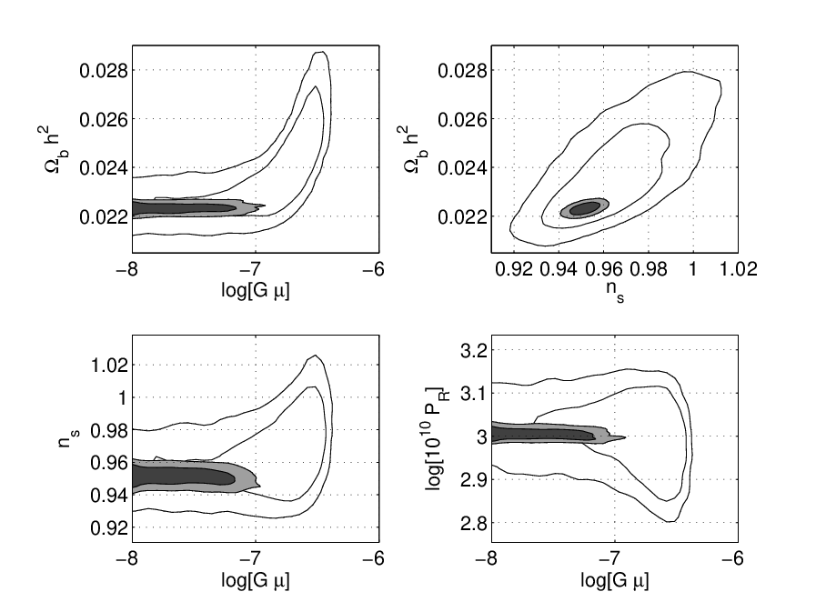
We have also performed the same analyses in the case of general and a similar qualitative picture emerges. The constraints on the parameters are summarized in Table 2, and Fig.1. The important difference from the case is that a much larger range of is allowed, albeit a very narrow one for each value of as suggested by (II.10). In this case, the constraint on is intimately related to that imposed by the data on .
| Parameter | Without | With |
| - | ||
| - | ||
| - | ||
| - |


It is clear that the inclusion of the string component has a non-trivial effect on the allowed likelihood surfaces. In this case larger values of are allowed with a limit of at confidence level, but with values being typically requiring significant () values of . There are upper limits , and .
III.2 Future constraints
The present constraints will be improved on by future CMB experiments, in particular the forthcoming ESA PLANCK mission bluebook. In order to quantify the likely improvement on the parameters discussed above, we assume that the observed CMB power spectrum is the sum of the underlying (which may or may not contain a string contribution) and an isotropic noise variance . We compute the error on the estimate of , which in turn gives confidence limits on the cosmological parameters, using the full-sky CMB likelihood function (see for example, ref. Lewis:2006ym). This is more accurate than Fisher matrix approaches if the posterior distribution is significantly non-Gaussian, which is certainly true for the models considered here.
We use the same noise properties as in ref. Lewis:2006ym, namely for the temperature and for the E-mode polarization signal, with a Gaussian beam width of 7 arcminutes. We assume an effective sky coverage , which acts as an ‘fudge’ factor in the full sky likelihood to approximate the partial sky case.
First, it is instructive to consider forecasted limits on from PLANCK, independent of any specific inflationary model. To do this, we use a fiducial set of ’s corresponding to the current standard 6 parameter fit CDM model Spergel:2006hy. For the MCMC analysis we then use as an additional free parameter, and so can provide upper limits assuming the underlying model has no string contribution.
The results of this are shown in Fig 2. For comparison, we have also included equivalent results for WMAP which were obtained in earlier work Battye:2006pk. There is a notable reduction in the range can take due to the increased sensitivity and resolution of PLANCK. Furthermore, the degeneracy between and other parameters, such as and is broken. For WMAP, we found a confidence upper bound of ; for the simulated PLANCK data this is reduced to .
We now assess the improved constraints on brane inflation models using simulated PLANCK data. For the fiducial set of input ’s we use the best fit parameters from a brane inflation model with . These parameters are similar to the standard CDM values used above, with the exception that is slightly higher (=0.967). The results of the analysis are shown in Fig. 3. In the case where we do not include the string contribution, the derived value of can again exceed . The constraint on is improved due to the tightening of that on with the confidence upper limit being reduced to . Including the string contribution does not modify constraints on and , but provides more stringent limits on and . The confidence upper limits for these parameters are reduced to and . The 4 order of magnitude improvement in the constraint on is due to the fact that .


We note that in addition to constraints from the TT, EE and TE, it is possible to constrain or even detect the effect of cosmic strings using the BB spectrum. It was suggested in ref. Battye:2006pk that maximum amplitude of the power spectrum for a model compatiable with the present data is at . Similar conclusions were found in ref. Bevis:2007qz.
IV Implications for the scalar-to-tensor ratio
The most significant implications of these results are for the possible values of allowed within such scenarios. From the expression for the scalar amplitude (II.5) and the tensor-to-scalar ratio (II.7)
| (IV.1) |
Since (II.8), we see that an upper bound on the string tension is also an upper bound on and therefore on . For , one finds
| (IV.2) |
where we have reinstated , the number of antibranes, as a parameter. Hence, if there is a limit of order imposed by the CMB data, then . If we assume, as we have done in the rest of the paper that , then there is a limit on the value of for any brane inflation model of this kind which is well below that which is likely to be observed by even the most ambitious CMB polarization instruments being considered, and it would require large values of to make this possible. Although the argument above applies strictly only to the , similar arguments can be made for low where inflation takes place in the slow-roll regime. This is interesting since other model dependent limits on have been considered in the literature Baumann:2006cd; Kallosh:2007wm.
For models of brane inflation involving mobile brane moving down warped throats, there is another upper limit on which can be derived from the upper bound on the inflaton field. The inflaton field is identified by the brane-antibrane separation and it cannot exceed the geometric limit imposed by size of the compactification manifold. One finds that Baumann:2006cd where the integer is the total brane charge which generates the warped geometry. Using the above geometric bound on the values of the inflaton, one can show that for warped brane inflation models. Since the supergravity approximation is valid in the large limit, , this seems to predict a very small amplitude for tensor modes. When compared with our bound from cosmic strings , which applies to the simple model (II.1), the above limit is stricter if . We conclude, therefore, that our observational limit its compatible with these theoretical arguments.
In the simplest brane inflation model featuring moduli stabilization Kachru:2003aw the value of can be related to the gravitino mass, . Such a model is essentially a single-field slow-roll model in which inflation occurs along a trough in the potential. The non-perturbative effects responsible for stabilizing the volume modulus generate an Anti-de-Sitter minimum, and the de-Sitter minimum is obtained by adding antibranes whose (warped) tension contribute a positive term to the overall value of the potential. The presence of the antibranes breaks supersymmetry, the breaking scale being set by the brane tension. Hence, one finds that the Hubble parameter during inflation is , which implies that , that is the energy scale of inflation, is the geometric mean of and . For the most commonly used gravitino mass the tensor modes are not observable, since this implies . For these small values of , , which is a much stronger bound than the one derived from cosmic strings here. Conversely, if this gravitino bound applies, the observation of tensor modes and cosmic strings will not be feasible in any realistic experiments. We emphasize, however, that not all models are constrained this way. For example in models where the uplifting is achieved by a racetrack superpotential Kallosh:2004yh, the gravitino mass is not related to the uplifting energy, and therefore the bound discussed above no longer applies.
V Discussion and conclusions
In this paper we have presented limits and constraints on the parameters (and derived parameters) of brane inflation models in the slow-roll regime when a cosmic string component is included in the fitting. Important aspects of the results are an increased range of acceptable values of , limits on , which is related to the volume of the internal space, the inflaton mass parameter and a constraint on the value of irrespective of any theoretical considerations with the consequent implications for .
We note that one way out of the bounds which we have discussed here is to consider the large regime, where there are again viable inflationary models Bean:2007hc. These models fall in the category of inflationary models with general speed of sound studied in Peiris:2007gz. In this case fast-roll inflation is possible due to the kinetic term actually being of the Dirac-Born-Infeld type (DBI) Silverstein:2003hf; Alishahiha:2004eh; Kecskemeti:2006cg. This modifies some of the preceding discussion. The Lagrangian for DBI inflation is
| (V.1) |
where the function depends on the throat geometry and the potential would be given by (II.9).
In this case, the expression for the scalar-to-tensor ratio is modified to where the parameter is defined as a generalized slow-roll parameter and the speed of sound is
| (V.2) |
Since one might think that would be small, however can be much larger in fast roll models. This was emphasized in ref. Bean:2007hc who also pointed out in the case where is small the non-Gaussianity of the density fluctuations, quantified by , would be particularly high due to consistency relation Lidsey:2006ia
| (V.3) |
which was derived in the equilateral triangle limit in momentum space.
As increases in the slow-roll 11 1 Simultaneously with our work, Ref.Bean:2007eh appeared where an alternative model, the so-called infrared DBI brane inflation, is compared with observations. For this class of models an even stronger bound on the cosmic string tension is found, . the value of increases beyond that which is compatible with the data. However, at some value of the effects of the DBI kinetic term kick in and the potential (II.9) becomes dominated by the term . Hence and are those of simple Klein-Gordon field, albeit modified by . This breaks the link between and , and therefore the constraints discussed in the previous sections only apply in the slow roll regime.
We note that all the brane inflation models constructed so far require some amount of fine-tuning to work. In the present case, the tuning corresponds to the value of being low. The effects of moduli stabilization have led to a large value of the parameter, making fine-tuning necessary in models of F-term inflation Kachru:2003sx; McAllister:2005mq. D-term inflation models do not suffer form the same -problem but threshold corrections to the superpotential Berg:2004ek; Berg:2005ja generate a large mass for the inflaton, making fine-tuning necessary in these models as well. A possible way to alleviate the fine-tuning problem is made possible by a remarkable property of a class of multi-brane models Cline:2005ty. Usually one balances the effect of the volume stabilization mechanism against the Coulombic brane-antibrane interaction to obtain a potential with a flat enough region to support inflation Burgess:2004kv. The model requires a fine balancing of the two effects. For generic values of the parameters the potential will either be too steep, or it will feature a local de-Sitter minimum where the mobile branes being separated from the antibranes by a potential barrier. However, if one or more branes tunnel out of the local minimum and annihilates with the antibranes, the height of the barrier decreases, and for a critical number of branes it disappears, resulting in a monotonic but almost flat potential. Inflation then proceeds via slow-roll as the remaining branes roll towards the antibranes stuck at the bottom of the warped throat. We will investigate this type of model using the techniques applied here in a future study.
A similar, but complementary study, to ours for the case but not including the string component has been performed in ref. Lorenz:2007ze. In order to get meaningful constraints they applied the bound on the exit scale as suggested in ref.Baumann:2006cd which is discussed in section IV. This study is relevant to the domain where the string tension is weakened by a large number of antibranes. We estimate that if these constraints will apply.
Finally we comment that there may be limits on which come from pulsar timing if the cosmic string network achieves scaling by the creation of loops and the subsequent emission of radiation (see ref. Caldwell:1996en and references therein). We caution that these should be considered to be less robust since they are more strongly effected by the small-scale dynamics, such as loop formation, of the cosmic string network. This is not completely understood in the case of standard cosmic strings in 3+1 dimensions; the situation with respect to the higher dimension cosmic strings is even less clear. Nonetheless, limits on the energy density in gravitational waves, , have substantially improved in recent times. Probably the most reliable limit is at frequencies Jenet:2006sv. Limits on from such a bound were considered in ref. Battye:2006pk and they are dependent on the loop production size relative to the horizon . If then is excluded and hence the limit from CMB anisotropy is strongest, whereas for one finds that is excluded, which would be tighter than the CMB limit for . It is clear that an improved understanding of the loop production mechanism coupled with expected improvements in the bound on could lead to a more powerful constraint than is expected from PLANCK.
References
- (1) G. F. Smoot et al., “Structure in the COBE differential microwave radiometer first year maps,” Astrophys. J. 396 (1992) L1.
- (2) D. N. Spergel et al. [WMAP Collaboration], “Wilkinson Microwave Anisotropy Probe (WMAP) three year results: Implications for cosmology,” Astrophys. J. Suppl. 170 (2007) 377 [arXiv:astro-ph/0603449].
- (3) G. R. Dvali and S. H. H. Tye, “Brane inflation,” Phys. Lett. B 450 (1999) 72 [arXiv:hep-ph/9812483].
- (4) C. P. Burgess, M. Majumdar, D. Nolte, F. Quevedo, G. Rajesh and R. J. Zhang, “The inflationary brane-antibrane universe,” JHEP 0107, 047 (2001) [arXiv:hep-th/0105204].
- (5) J. Garcia-Bellido, R. Rabadan and F. Zamora, “Inflationary scenarios from branes at angles,” JHEP 0201, 036 (2002) [arXiv:hep-th/0112147].
- (6) A. Sen, “Tachyon condensation on the brane antibrane system,” JHEP 9808, 012 (1998) [arXiv:hep-th/9805170]. E. Witten, “D-branes and K-theory,” JHEP 9812, 019 (1998) [arXiv:hep-th/9810188]. P. Horava, “Type IIA D-branes, K-theory, and matrix theory,” Adv. Theor. Math. Phys. 2, 1373 (1999) [arXiv:hep-th/9812135]. M. Majumdar and A. Christine-Davis, “Cosmological creation of D-branes and anti-D-branes,” JHEP 0203, 056 (2002) [arXiv:hep-th/0202148].
- (7) S. Sarangi and S. H. H. Tye, “Cosmic string production towards the end of brane inflation,” Phys. Lett. B 536, 185 (2002) [arXiv:hep-th/0204074]. N. T. Jones, H. Stoica and S. H. H. Tye, “The production, spectrum and evolution of cosmic strings in brane inflation,” Phys. Lett. B 563, 6 (2003) [arXiv:hep-th/0303269]. N. Barnaby, A. Berndsen, J. M. Cline and H. Stoica, “Overproduction of cosmic superstrings,” JHEP 0506, 075 (2005) [arXiv:hep-th/0412095].
- (8) S. Kachru, R. Kallosh, A. Linde, J. M. Maldacena, L. McAllister and S. P. Trivedi, “Towards inflation in string theory,” JCAP 0310 (2003) 013 [arXiv:hep-th/0308055].
- (9) P. Kraus and F. Larsen, “Boundary string field theory of the DD-bar system,” Phys. Rev. D 63, 106004 (2001) [arXiv:hep-th/0012198]. T. Takayanagi, S. Terashima and T. Uesugi, “Brane-antibrane action from boundary string field theory,” JHEP 0103, 019 (2001) [arXiv:hep-th/0012210].
- (10) C. Contaldi, M. Hindmarsh and J. Magueijo, “The power spectra of CMB and density fluctuations seeded by local cosmic strings,” Phys. Rev. Lett. 82 (1999) 679 [arXiv:astro-ph/9808201].
- (11) R. A. Battye and J. Weller, “Cosmic structure formation in hybrid inflation models,” Phys. Rev. D 61 (2000) 043501 [arXiv:astro-ph/9810203].
- (12) M. Wyman, L. Pogosian and I. Wasserman, “Bounds on cosmic strings from WMAP and SDSS,” Phys. Rev. D 72 (2005) 023513 [Erratum-ibid. D 73 (2006) 089905] [arXiv:astro-ph/0503364].
- (13) U. Seljak, A. Slosar and P. McDonald, “Cosmological parameters from combining the Lyman-alpha forest with CMB, galaxy clustering and SN constraints,” arXiv:astro-ph/0604335.
- (14) N. Bevis, M. Hindmarsh, M. Kunz and J. Urrestilla, “CMB power spectrum contribution from cosmic strings using field-evolution simulations of the Abelian Higgs model,” arXiv:astro-ph/0605018.
- (15) R. A. Battye, B. Garbrecht and A. Moss, “Constraints on supersymmetric models of hybrid inflation,” JCAP 0609 (2006) 007 [arXiv:astro-ph/0607339].
- (16) N. Bevis, M. Hindmarsh, M. Kunz and J. Urrestilla, “Fitting CMB data with cosmic strings and inflation,” arXiv:astro-ph/0702223.
- (17) I. R. Klebanov and M. J. Strassler, “Supergravity and a confining gauge theory: Duality cascades and chiSB-resolution of naked singularities,” JHEP 0008, 052 (2000) [arXiv:hep-th/0007191].
- (18) H. Firouzjahi and S. H. Tye, “Brane inflation and cosmic string tension in superstring theory,” JCAP 0503 (2005) 009 [arXiv:hep-th/0501099].
- (19) L. Pogosian and T. Vachaspati, “Cosmic microwave background anisotropy from wiggly strings,” Phys. Rev. D 60 (1999) 083504 [arXiv:astro-ph/9903361].
- (20) A. Albrecht, R. A. Battye and J. Robinson, “The case against scaling defect models of cosmic structure formation,” Phys. Rev. Lett. 79 (1997) 4736 [arXiv:astro-ph/9707129]; R. A. Battye, J. Robinson and A. Albrecht, “Structure formation by cosmic strings with a cosmological constant,” Phys. Rev. Lett. 80 (1998) 4847 [arXiv:astro-ph/9711336]; A. Albrecht, R. A. Battye and J. Robinson, “A detailed study of defect models for cosmic structure formation,” Phys. Rev. D 59 (1999) 023508 [arXiv:astro-ph/9711121].
- (21) U. Seljak and M. Zaldarriaga, “A Line of Sight Approach to Cosmic Microwave Background Anisotropies,” Ap. J 469 (1996) 437 [arXiv:astro-ph/9603033].
- (22) A. Lewis, A. Challinor and A. Lasenby, “Efficient Computation of CMB anisotropies in closed FRW models,” Ap. J 538 (2000) 473 [arXiv:astro-ph/9911177].
- (23) S. Kachru, R. Kallosh, A. Linde and S. P. Trivedi, “De Sitter vacua in string theory,” Phys. Rev. D 68 (2003) 046005 [arXiv:hep-th/0301240].
- (24) L. McAllister, “An inflaton mass problem in string inflation from threshold corrections to volume stabilization,” JCAP 0602, 010 (2006) [arXiv:hep-th/0502001].
- (25) O. DeWolfe and S. B. Giddings, “Scales and hierarchies in warped compactifications and brane worlds,” Phys. Rev. D 67, 066008 (2003) [arXiv:hep-th/0208123].
- (26) C. P. Burgess, J. M. Cline, H. Stoica and F. Quevedo, “Inflation in realistic D-brane models,” JHEP 0409, 033 (2004) [arXiv:hep-th/0403119].
- (27) M. Berg, M. Haack and B. Kors, “Loop corrections to volume moduli and inflation in string theory,” Phys. Rev. D 71, 026005 (2005) [arXiv:hep-th/0404087].
- (28) M. Berg, M. Haack and B. Kors, “String loop corrections to Kaehler potentials in orientifolds,” JHEP 0511, 030 (2005) [arXiv:hep-th/0508043].
- (29) M. Berg, M. Haack and B. Kors, “On the moduli dependence of nonperturbative superpotentials in brane arXiv:hep-th/0409282.
- (30) D. Baumann, A. Dymarsky, I. R. Klebanov, L. McAllister and P. J. Steinhardt, Phys. Rev. Lett. 99, 141601 (2007) [arXiv:0705.3837 [hep-th]].
- (31) D. Baumann, A. Dymarsky, I. R. Klebanov and L. McAllister, arXiv:0706.0360 [hep-th].
- (32) A. Lewis and S. Bridle, “Cosmological parameters from CMB and other data: a Monte-Carlo approach,” Phys. Rev. D 66 (2002) 103511 [arXiv:astro-ph/0205436].
- (33) G. Hinshaw et al., “Three-Year Wilkinson Microwave Anisotropy Probe (WMAP) Observations: Temperature Analysis,” arXix:astro-ph/0603451.
- (34) L. Page et al., “Three Year Wilkinson Microwave Anisotropy Probe (WMAP) Observations: Polarization Analysis,” arXix:astro-ph/0603450.
- (35) D. H. Lyth, “What would we learn by detecting a gravitational wave signal in the cosmic microwave background anisotropy?,” Phys. Rev. Lett. 78 (1997) 1861 [arXiv:hep-ph/9606387].
- (36) G. Efstathiou and K. J. Mack, “The Lyth Bound Revisited,” JCAP 0505, 008 (2005) [arXiv:astro-ph/0503360].
- (37) Planck: The Scientific Programme, ESA-SCI (2005) 1.
- (38) A. L. Lewis, J. Weller and R. A. Battye, “The Cosmic Microwave Background and the Ionization History of the Universe,” MNRAS 373 (2006) 561 [arXiv:astro-ph/0606552].
- (39) N. Bevis, M. Hindmarsh, M. Kunz and J. Urrestilla, Phys. Rev. D 76, 043005 (2007) [arXiv:0704.3800 [astro-ph]].
- (40) D. Baumann and L. McAllister, “A microscopic limit on gravitational waves from D-brane inflation,” Phys. Rev. D 75 (2007) 123508 [arXiv:hep-th/0610285].
- (41) R. Kallosh and A. Linde, “Testing String Theory with CMB,” JCAP 0704, 017 (2007) [arXiv:0704.0647 [hep-th]].
- (42) R. Kallosh and A. Linde, “Landscape, the scale of SUSY breaking, and inflation,” JHEP 0412, 004 (2004) [arXiv:hep-th/0411011].
- (43) R. Bean, S. E. Shandera, S. H. Henry Tye and J. Xu, “Comparing Brane Inflation to WMAP,” JCAP 0705 (2007) 004 [arXiv:hep-th/0702107].
- (44) H. V. Peiris, D. Baumann, B. Friedman and A. Cooray, “Phenomenology of D-Brane Inflation with General Speed of Sound,” arXiv:0706.1240 [astro-ph].
- (45) E. Silverstein and D. Tong, “Scalar speed limits and cosmology: Acceleration from D-cceleration,” Phys. Rev. D 70, 103505 (2004) [arXiv:hep-th/0310221].
- (46) M. Alishahiha, E. Silverstein and D. Tong, “DBI in the sky,” Phys. Rev. D 70, 123505 (2004) [arXiv:hep-th/0404084].
- (47) S. Kecskemeti, J. Maiden, G. Shiu and B. Underwood, “DBI inflation in the tip region of a warped throat,” JHEP 0609, 076 (2006) [arXiv:hep-th/0605189].
- (48) J. E. Lidsey and D. Seery, “Primordial non-Gaussianity and gravitational waves: Observational tests of brane inflation in string theory,” Phys. Rev. D 75, 043505 (2007) [arXiv:astro-ph/0610398].
- (49) R. Bean, X. Chen, H. V. Peiris and J. Xu, “Comparing Infrared Dirac-Born-Infeld Brane Inflation to Observations,” arXiv:0710.1812 [hep-th].
- (50) J. M. Cline and H. Stoica, “Multibrane inflation and dynamical flattening of the inflaton potential,” Phys. Rev. D 72 (2005) 126004 [arXiv:hep-th/0508029].
- (51) L. Lorenz, J. Martin and C. Ringeval, “Brane inflation and the WMAP data: a Bayesian analysis,” arXiv:0709.3758 [hep-th].
- (52) R. R. Caldwell, R. A. Battye and E. P. S. Shellard, “Relic gravitational waves from cosmic strings: Updated constraints and opportunities for detection,” Phys. Rev. D 54, 7146 (1996) [arXiv:astro-ph/9607130].
- (53) F. A. Jenet et al., “Upper bounds on the low-frequency stochastic gravitational wave background from pulsar timing observations: Current limits and future prospects,” Astrophys. J. 653, 1571 (2006) [arXiv:astro-ph/0609013].