THE COMPLEX OF PANT DECOMPOSITIONS OF A SURFACE
Abstract.
We exhibit a set of edges (moves) and 2-cells (relations) making the complex of pant decompositions on a surface a simply connected complex. Our construction, unlike the previous ones, keeps the arguments concerning the structural transformations independent from those deriving from the action of the mapping class group. The moves and the relations turn out to be supported in subsurfaces with (where is the genus and is the number of boundary components), illustrating in this way the so called Grothendieck principle.
Key words and phrases:
Pant decomposition complex, mapping class group, complex of curves.1991 Mathematics Subject Classification
Primary 57M50; Secondary 57M20, 30F601. Introduction
Let be a connected, compact, oriented surface of genus with boundary components (). In order to describe an algebraic or geometric object , it is often convenient to represent as the result of gluing together several simple pieces, which should be surfaces with boundary.
This happens for example in the study of the mapping class group (whose presentation may be obtained starting from those of the mapping class group of some simple subsurfaces, as proved in [4]), in the pantwise construction of hyperbolic structures (Fenchel-Nielsen construction) and in the construction of modular functors (defined by gluing the vector spaces associated to simpler subsurfaces, provided they satisfy some gluing axiom).
Depending on the situation, it is convenient to choose the building blocks for our surfaces from different Lego boxes: one may choose, for example, a big Lego box (the grande boite in [9]), whose pieces are all the spheres with any number of boundary components, or maybe a smaller Lego box, containing only spheres with at most three boundary components. In many cases, a cheap Lego box, made of identical pieces (namely spheres with three boundary components or hexagons) may be sufficient.
No matter which box one chooses, it is evident that each surface admits an infinite number of different decompositions with pieces out of that box (see for instance Figure 1).

Thus, if one wants to describe an object using a decomposition of (i.e. computing as a ), in order for this object to be well defined it is necessary to construct canonical isomorphisms between the objects computed starting from different decompositions, i.e. to construct isomorphisms
where and are any two different decompositions of .
For instance, coming back to the cases mentioned before: while studying the mapping class group it turns out that different “slicing” of produce different presentations for , and we look for a procedure to get any presentation from any other; while constructing hyperbolic structures, different pant decompositions lead to the description of different charts of the atlas of the Teichmüller space of , and we look for the change of chart; while building a modular functor, different ways of sewing result in different bases for the vector space associated to , and we need to write down the matrices giving the change of basis (duality matrices in [16]).
Therefore, once the Lego box is fixed, we have to describe the set of all the decompositions of a surface into pieces from that Lego box, considered up to isotopy, and the set of all the transformations between different (non-isotopic) decompositions. More precisely, our aim is to exhibit:
- elementary moves,
-
such that we can go from a given decomposition to any other through a sequence of these moves;
- defining relations,
-
describing when a sequence of elementary moves applied to a decomposition yields the same decomposition.
Following the philosophy introduced by Hatcher and Thurston in their pioneering paper [11], such problem can be reformulated as follows: we consider all the decompositions of the surface up to isotopy, as the vertices of a 2-dimensional CW complex ; then we put an edge between two vertices if the corresponding decompositions are related by one of our candidate moves, and we cup off a loop with a 2-cell if the corresponding sequence of moves is one of our candidate relations. Hence we are reduced to check that is simply connected. Indeed, this complex is connected if and only if the set of our candidates moves is complete. Moreover, it is simply connected if and only if any relation between elementary moves follows from the ones we have cupped off. Actually in [11] the focus is on the cut system complex , but in the appendix the authors suggest that the same program could be carried over to the case of pant decompositions.
The pant decomposition complex was studied in [16] by Moore and Seiberg. Unfortunately, their proof of the connectedness and simply connectedness of the so built complex contains some serious gaps. In particular, it is based on the knowledge of an explicit presentation for the mapping class groups , which was then unknown. Indeed, at the moment they were writing (1989), the only known finite presentations were those of the modular groups and .
The mapping class group of the surface we are examinating enters the playground since the elements of this group act as transformations on the set of the decompositions of : for instance, the decomposition shown in the right hand picture of Figure 1 is obtained from the one in the center by a Dehn twist along the dotted curve. Anyway, not all transformations between decompositions are elements of the mapping class group: for instance, the decomposition shown in the left hand picture of Figure 1 cannot be transformed into the center one (nor into the right one) by any homeomorphism of . Therefore, the set of transformations between different decompositions of the surface contains a core, that is the mapping class group , and something additional: the idea in [16] is to get rid of this “extra part” and eventually come to the study of , which is what Moore and Seiberg could not carry out.
More recently, this problem has been overcome by using the Cerf theoretic techniques introduced in [11], either directly [6, 10] or passing through a projection on the cut systems complex [2].
In this paper, we come back to the original Moore and Seiberg’s approach and fill in the gaps, exploiting the presentations of the mapping class groups that we have at present.
Indeed, in [8], Gervais provides a presentation of , in terms of Dehn twists. Another presentation, as quotients of Artin groups, is described by Matsumoto in [14] for and then generalized to the case of by Labruère and Paris in [12].
A general machinery for getting presentations of the mapping class groups in any preferred “style” (for example in terms of Dehn twists or as quotients of Artin groups) is given in [4]. The procedure introduced in that paper takes as input the well known presentations for the sporadic surfaces (, , and ) according to some “style” and returns a presentation in the same “style” for every . Such flexibility makes this last approach suitable for obtaining different descriptions of the complex we may need in different contexts.
The paper is organized as follows. Section 2 contains the first definitions and the main tools. The construction of the complex is subdivided into two independent steps. Given a surface , in Section 3 we consider a 2-dimensional, finite, simply connected CW complex , whose vertices are in one-to-one correspondence with the combinatorial structures of pant decompositions of , i.e. with the -equivalence classes of such decompositions. Then, in Section 4, by using a presentation of , we construct an infinite simply connected complex codifying all the pant decompositions on and the transformations between them, that is the desired .
When we started thinking of this Lego-Teichmüller game, our aim was to understand something new about a Grothendieck conjecture on the subject (see [9]). In our context this conjecture can be expressed, roughly speaking, as follows. Take the family of all the complexes and stack them in levels, putting at level all the with . Then, to describe the whole tower of complexes, it is sufficient to describe its first and second floor, i.e. the complexes with , that are precisely the ones of the sporadic surfaces , , and .
It is worth noticing that we obtained this Grothendieck principle for the mapping class groups as a byproduct, in [4]. Namely, we proved that the generators and the relations which are needed to present the mapping class group of any surface are supported in subsurfaces living at the first and second Grothendieck floor. Combining this result with the new ones described in the present paper, we are now able to prove the Grothendieck conjecture in the above stated form.
2. First definitions and main tools
Let be a connected, compact, oriented surface, of genus with boundary components. A pant decomposition of is a decomposition of the surface into a finite number of pants, determined by a collection of disjoint simple closed curves in the interior of . We recall that a pant is a closed disk with two smaller open disks removed, i.e. the surface . As usual, the family of curves and therefore the induced pant decomposition are always considered up to isotopy.

More precisely, let be a collection of pairwise disjoint closed loops on . We denote by the natural compactification of (obtained compactifying each component by the addiction of three boundarycurves), and by the continuous map induced by the inclusion of into .
Definition 1.
We say that the family determines a pant decomposition of if each component of is a pant, or equivalently if consists of components, each of which is homeomorphic to the interior of a pant.
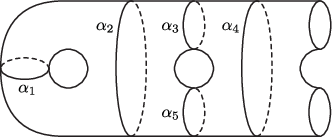
It can be easily shown that admits a pant decomposition provided
Moreover, the integers and are uniquely determined, and they are given by
where is the Euler characteristic of the surface .
Let be a connected component of (notations as above). We say that a boundary curve of is an exterior boundary curve if is a boundary component of . For each curve in the family there are two distinct boundary curves in such that , and two possibilities arise: either and are boundary curves of the same connected component of (like in Figure 3), or is a boundary component of and is a boundary component of a different connected component (like in Figure 3). In the first case we call a non-separating limit curve of , while in the second case we call it a separating limit curve of and .
We denote by the mapping class group of , i.e. the group of the isotopy classes of orientation preserving homeomorphisms which fix pointwise the boundary of . Clearly, we have an induced action of on the set of the pant decompositions of . We call -equivalent two pant decompositions that can be obtained from one another by such action.
Definition 2.
A combinatorial structure of pant decompositions of is a class of -equivalence of pant decompositions on .
Now we can state the following proposition, whose proof is trivial.
Proposition 3.
Let and be two isotopy classes of curves defining pant decompositions of . Then the two pant decompositions belong to the same combinatorial structure if and only if there exists a one-to-one correspondence between the components of and those of and there exists a permutation such that, for every pair where is any component of and the corresponding component of , we have:
- 1)
if is an exterior boundary curve of there exist an exterior boundary curve of such that (i.e. and have the same boundary components);
- 2)
if is a separating (resp. non-separating) limit curve of , then is a separating (resp. non-separating) limit curve of .
In the light of the previous proposition, once a numbering of the boundary components of is fixed, any combinatorial structure of pant decompositions of can be encoded by its dual graph. This graph has trivalent vertices corresponding to pants, and univalent vertices corresponding to the boundary components. Moreover, the univalent vertices are labelled by according to the fixed numbering of the boundary components of .
The next proposition will be used as a criterion for the simply connectedness of the complexes we are going to construct.
Proposition 4.
Let be a surjective cellular map between 2-dimensional CW complexes. Suppose the following conditions are satisfied:
- 1)
for any vertex , the fiber is connected and simply connected in ;
- 2)
for any oriented edge in and any two liftings and of in , there exist two paths in the fiber and , in the fiber , such that the square
![[Uncaptioned image]](0710.1483v2/diagram1.png)
is contractible in .
Then, if is simply connected, is simply connected as well.
The proof of this proposition is straightforward, and it is left to the reader.
3. The combinatorial structures of pant decompositions
This section is devoted to the construction of a simply connected complex whose vertices represent the combinatorial structures of pant decompositions of or equivalently their dual graphs, as we said in the previous section. Moreover, in the last subsection we will lift the complex to another one, denoted by , codifying all of decorated combinatorial structures, i.e. the combinatorial structures of pant decompositions whose curves are ordered. This is a technical tool which will be needed in Section 4.
We define to be the set of all connected graphs with univalent vertices, also called free ends, and trivalent vertices. A standard computation shows that each of these graphs has edges, connecting a free end to a trivalent vertex, and the remaining connecting two (possibly coinciding) trivalent vertices.
On such graphs we consider the local move shown in Figure 4, that we call combinatorial move, according to the literature, as it can be thought as the fusion of two adjacent trivalent vertices followed by the inverse of a similar fusion. We warn the reader that the graphs in this picture, as well as in the following ones, should be considered as abstract graphs, regardless of their planar representation.

The picture means that the graph is unchanged outside a regular neighborhood of an edge between two distinct trivalent vertices, while such edge is replaced with a new edge , connecting two new trivalent vertices. To be more precise, let and be the trivalent vertices connected by the edge on which we perform the move. Then, for each , there are two (possibly coinciding) edges other than having as a vertex. We label those connected to by and , and those connected to by and . Thus, the starting graph represents the coupling . Therefore, for each edge between trivalent vertices there are exactly two possible ways to perform the move (i.e. two possible results for the move), corresponding to the two possible changes of coupling:
The move is oriented and in the pictures we mark the starting edge on which the move is performed by surrounding it by a grey region.
To emphasize that the move can be realized as the contraction of the edge followed by the inverse of a similar contraction of the edge , we will label the arrows representing moves by the corresponding intermediate graphs.


Now, we define to be the complex having as the set of vertices, an undirected edge connecting any two vertices which are related by a combinatorial move, and the following 2-cells:
Coherently with what we have done for the edges, we consider only one two cell for each loop of edges as in the Figures, even if the same loop may be represented by different sequences of moves.
Remark 5.
Notice that triangles appear for , squares and pentagons show up when , while bigons are required for .
Remark 6.
The arrows appearing in the pictures do not represent an orientation for the edges, but they are only intended to specify the oriented move we are considering.
The main result of this section is the following.
Theorem 7.
The complex , with , is simply connected.
The proof takes the next two subsections and proceeds by an induction scheme based on the diagram below, where the complexes are staked in layers corresponding to the value of .
![[Uncaptioned image]](0710.1483v2/diagram2.png)
The base for the inductive argument is provided by the two complexes and , which both consist of a single vertex and are therefore trivially connected and simply connected.
In Subsection 3.1 we define the maps and show that they satisfy the hypotheses of Proposition 4, in order to derive the simply connectedness of from that of (Proposition 8). On the other hand, the maps are defined in Subsection 3.2 and are used to prove that the simply connectedness of implies that of (Proposition 9).
3.1. Reducing the number of boundary components
We start by defining the map
If is a vertex of , is the graph obtained from by contracting the last free end as in Figure 9: the result is a connected graph with free ends in the set and trivalent vertices, i.e. a vertex of .

As far as the edges are concerned, with the notations introduced at the beginning of this section, we have two possibilities: either or . In the first case, is defined as the move between and . In the second case, being , we can define , as depicted in Figure 10.

Finally we define on the 2-cells in the following way. If sends the boundary of a -cell of onto the boundary of a -cell of having the same shape, then sends the -cell of in the corresponding one of . Otherwise, it may happen that an edge of the -cell collapses to a vertex of , as in Figure 10. If this happens for a bigon or a triangle, then sends the entire boundary to the same vertex, and we send the 2-cell itself to such vertex. On the other hand, if it happens for a square or a pentagon, then the image of the boundary reduces to an edge, and we send all the 2-cell to such an edge.
The map defined in this way is obviously cellular and surjective both on vertices and on edges. To see that it is also surjective on -cells, we observe that each -cell of is the image of a -cell of of the same shape. In fact, the moves on the boundary of a -cell of always leave a free edge on which the new trivalent vertex can be created, to get the boundary of a -cell of such that no edge collapses.
Now, we use to get the following inductive step for the proof of Theorem 7.
Proposition 8.
If the complex is simply connected, then also is simply connected, for every and such that .
Proof.
The thesis follows by applying Proposition 4 to the map , once we prove that the required conditions concerning the preimages of vertices and edges are fulfilled.
Claim 1. The fiber over each vertex is connected and simply connected in .
Let be a vertex of . Then the vertices of consists of all the graphs with free ends obtained from by inserting an edge with one free end labelled by and the other end creating a new trivalent vertex along any of the edges of , which is therefore split into two edges (see Figure 11).

Notice that two vertices of span an edge in if and only if they are graphs obtained from by inserting the new edge on adjacent edges of , i.e. if and only if they can be obtained from one another by sliding the new trivalent vertex, from one edge of to the adjacent one, through their common trivalent vertex. As explained in Figure 12, this sliding is in fact an move performed on the marked edge. Then the connectedness of immediately follows from that of .

The above observation allows us to define a canonical projection from the 1-skeleton of to the graph , once they are barycentrically subdivided. Namely, we project any vertex of to the barycenter of the edge of split to get as a graph, and the barycenter of any edge of to the vertex of shared by the to edges of split to obtain respectively and . Then, we extend the projection to a cellular map between the two barycentric subdivisions in the obvious way.
Such projection induces a natural one-to-one correspondence between all the paths in and those paths in the barycentric subdivision of whose both ends are barycenters of edges of . Moreover, this correspondence respects composition and sends loops to loops.
We need to show that any loop in any fiber , with a vertex of , can be contracted in (by getting out of the fiber if needed). The proof is by induction on the length of .
The base of the induction is the case . In this case the loop corresponds to an move which, applied to a graph, produces a new graph equivalent to the original one. This happens when the -th vertex is attached onto two adjacent edges and of , possibly coinciding, which are equivalent by an automorphism of . Figure 13 shows how it is possible to contract such a loop, exploiting the fact that it is one of the three edges of a triangle, whose other two edges coincide.

For , the inductive step consists in proving that loop is contractible in , assuming that the same holds for all the loops of length in any fiber .

By means of the one-to-one correspondence introduced above, we can interpret as a loop of edges in .
The loop may retrace one of its edges, i.e. may contain an edge of the barycentric subdivision of followed by the same edge with the opposite orientation. This may happen in one of the two cases depicted in Figure 14. In the first situation, the retrace appears in as well, and may be canceled. The second situation represents a triangle in . By homotoping over the corresponding -cell, the retrace may be canceled.
After canceling all the retraces, we can assume that the length of and coincide.
Now, let us suppose that is not injective: this means that an edge of appears two times in the loop . If this is the case, then the loop can be decomposed into two loops of smaller length, inducing a similar decomposition on . By induction on the length we are done.
Finally, we are reduced to the case when is an injective loop, i.e. it is a circuit in (see Figure 15).

We choose a vertex of . is a vertex of , obtained from inserting a new edge with a free end in the point and the other end creating a new trivalent vertex on the edge . All the remaining vertices of are obtained from inserting the new edge on the edges of . Let us denote by the vertex which precedes and by the one following it (with respect to the orientation of ). Those vertices are obtained from by attaching the new edge on the two edges of adjacent to edge (see Figure 16).

At this point, we apply to all vertices in the move performed on the edge ( in the following), getting from each of them a graph belonging to . The graph has a circuit of length , and the vertices obtained above are those of the corresponding loop of ( in Figure 17).
The move which connects any pair of adjacent vertices in , together with the two moves departing from such vertices and with the move connecting their images in , bounds a DC square (see Figure 17).

Let us consider the pentagonal loop with vertices , , (all belonging to ), and (in ). As illustrated in Figure 18, such loop can be filled in with triangles and pentagons.

The -sided loop can therefore be homotoped to the -sided one, which is in turn contractible by the inductive hypothesis, from which the thesis follows.
Claim 2. The condition on the lifting of edges is satisfied.
Let be an edge of . Such is an move performed on an edge (with distinct endpoints) of : hence, has liftings to , as many as the number of edges in . Let and be two of these liftings. As is connected, there is a simple path in connecting to . The graph is obtained from by inserting a new trivalent vertex on an edge which is different from , and connecting it with the new free end . The path consists of consecutive moves in the fiber, i.e. consecutive slidings of the new trivalent vertex. We concentrate on the first edge of , the one departing from . Such edge represents a sliding of the new vertex from edge to edge , through the vertex they have in common (i.e. it is an move in the fiber ): denoted by the resulting graph, still belonging to , three possibilities are given:
- (i)
and are disjoint;
- (ii)
and intersect at a vertex, and ;
- (iii)
and intersect at a vertex, and .
In the first case, admits a lifting , and is obtained from with the same sliding used to get from . The two liftings of and the two slidings bound a DC square, and the resulting loop is therefore contractible.
In the second case, still admits a lifting , but to get from we need to perform two slidings along consecutive vertices. Then, the two liftings of and the three slidings bound a pentagon, and the resulting loop is once again contractible (see Figure 19).


In the third case, instead, does not support the move that lifts . However, if we slide further, by walking through the following edge in the path , we end up with a graph that supports the move. Denoted by the lifting of starting in , two possibilities are given: either the graph turns out to be related to by a single sliding, or two slidings are needed to get from . In the former case, the two liftings of and the three slidings still bound a pentagon, resulting in a contractible loop (see Figure 20). In the latter case, the two liftings and the four slidings give rise to an hexagon. Nevertheless, such an hexagon may be subdivided into triangles and pentagons, as shown in Figure 21, being therefore contractible.
The same argument applies to all consecutive edges of the path . We get this way a path in connecting to , and the loop bounded by , , and is contractible by construction. Hence Claim 2 is proved.
This concludes the proof of Proposition 8. ∎
3.2. Dealing with the closed case
A further step needed to prove Theorem 7, is the definition of a map
We define this map as follows. If is a vertex of , then is the graph obtained from by attaching its two free ends together, as shown in Figure 22. Such a graph turns out to have trivalent vertices and no free ends, i.e. it is a vertex of . Now, every edge of is an move connecting two graphs . Then there exists an move between and , and we define to be such a move. The definition of on the 2-cells is straightforward.

The map we have just defined is cellular. It allows us to obtain the second inductive step for the proof of Theorem 7.
Proposition 9.
If the complex is simply connected, then also is simply connected, for every .
Proof.
We observe that can be easily seen to be surjective, by the same argument used for the surjectivity of , except that here the free edge is the one to be cut to get liftings of cells. Then the connectedness of implies that of , and the proposition immediately follows from the following claim.
Claim 1. For any loop of edges in there exists a loop of edges in , such that is homotopic to in .
In order to prove this claim, we need another claim.
Claim 2. For any vertex of and any two vertices and in , there exists a path of edges in between and , such that the loop is homotopically trivial in .

We first prove Claim 1 assuming Claim 2. We choose a vertex of as the base point for the loop , and denote by the vertex of , which is obtained from by cutting it along an edge .
We choose as the basepoint of the lifting and consider the first edge of , i.e. the one departing from . Such edge is an move performed on an edge of . If , then we can lift the move to a move on . On the contrary, if then the move cannot be lifted to a move on the graph and we apply Claim 2 in order to connect with a different vertex of on which the move can be lifted.
We go on to construct our lifting, by following edge after edge and iterating the procedure described for the first edge.
In this way we end up with a path joining with some other vertex of and we can close it to get the desired loop by applying once again Claim 2. The scenario is that of Figure 23.
Then differs from only for the insertion of some homotopically trivial loops , one for each application of Claim 2. Therefore, is homotopic to as required by Claim 1.
Now we pass to prove Claim 2. Let and be obtained from respectively by cutting two different edges and .
If and share both the ends, then (see rightmost graphs in Figure 24) and there is nothing to prove.

Otherwise, if and do not share both ends but are still adjacent, then the fact that both can be cut without disconnecting ensures the existence of a simple path of edges in joining two different vertices of and , as in Figure 24. The same figure suggests how to construct the desired path as a sequence of liftings of moves performed in the order on the egdes of , followed by a sequence of liftings of their inverses in the reversed order. Then the loop turn out to be homotopically trivial by construction.
Finally, if and are not adjacent, then we consider a minimal path of edges in between a (trivalent) vertex of and a vertex of . By performing moves on the edges of in the order, we can drag until it coincides with . In this way we get a path of edges in connecting with a new graph where and are adjacent. Since neither nor can appear in , we can lift to paths and in respectively starting from and . Now, calling and the end points of these two paths in , we are reduced to the previous case. Therefore, we can find a path of edges between and such that the loop is contractible in . Then we put and observe that once again the loop is homotopically trivial by construction. ∎
3.3. The decorated combinatorial structures
As anticipated, we conclude this section with the construction of the complex , codifying all of decorated combinatorial structures, i.e. the combinatorial structures of pant decompositions whose curves are ordered.
Let be the set of all connected graphs with univalent vertices and trivalent vertices, equipped with an ordering of the edges connecting two trivalent vertices. For those graphs we may define a decorated move, naturally lifting the combinatorial move defined in Section 3, simply requiring that the new edge created by the move inherits its number by the old one. In order to emphasize that the move is performed on the -th edge, we denote it by . Moreover, if two decorated graphs are identical except for the ordering of the edges, which differ by a transposition , we connect them with an edge, labeled by . We complete the construction by adding 2-cells of three types: combinatorial, algebraic and mixed ones.
The combinatorial 2-cells translate in terms of decorated combinatorial structures the bigons, triangles, squares and pentagons of . Notice that the shape of the bigons and that of the pentagons change when lifted to the decorated setting, as depicted in Figure 25, while all the other combinatorial cells maintain their shape.

The algebraic -cells correspond to the relation in the group , thus they are squares , for any couple of different transpositions and in , where .
Finally, the mixed two cells are squares , telling that and moves commute.
The complex built like that has an obvious projection on , which is defined on the vertices by forgetting the ordering and extends to edges and 2-cells in a natural way. Proving that such map satisfies all the hypothesis of Proposition 4 is straightforward, and we leave it to the reader. The application of Proposition 4 thus ensures that is connected and simply connected.
4. The complex of pant decompositions
In this section we want to lift the complex to a new complex , whose vertices are in one-to-one correspondence with the pant decompositions of the surface . This result is achieved in two steps, described in the two subsections: first of all, we define a complex , whose vertices are in one-to-one correspondence with the decorated pant decompositions of , in such a way that the natural action of the mapping class group on the decorated pant decompositions extends to an action on and the quotient coincides with . Provided we take care that the natural projection satisfies the conditions of Proposition 4, the new complex turns out to be simply connected. Finally, we exploit the natural projection to prove that is simply connected as well.
4.1. The decorated pant decompositions
As anticipated in the introduction, we need now a presentation for all the mapping class groups. In order to produce such presentation, we use the results of [4]. In such paper a machinery for finding presentations is built; its input is a presentation for the mapping class group of the sphere with and boundary components, and for the torus with and boundary components (sporadic surfaces). Moreover, [4] also shows that such a machinery produces a presentation of any known “style”, provided the input is chosen according to the same “style”. In order to perform the explicit calculations shown in this section, it is convenient to use a presentation in terms of Dehn twists, described by Gervais in [7], that we may obtain with the above recalled method starting from the Dehn twist style presentations for the sporadic surfaces.
The generators in such a presentation are the Dehn twists along all simple closed curves in , while the relations belong to three simple types, braids, lanterns and chains.
Namely, we call braids the relations of the form
where the curves and are such that or (meaning they intersect in two points with algebraic intersection zero), and .


The vertices of have to be in a one to one correspondence with the (infinitely many) decorated pant decompositions of , i.e.
We now define a transformation between decorated pant decompositions, that we call again move. Let be the decorated pant decomposition given by an ordered family of curves (up to isotopy). Let us consider one of these curves, , and let be any curve on such that and is still a decorated pant decomposition. The move is defined as the transformation
In order to emphasize that such move is performed on the -th curve of , we denote it by .
The move, depicted in Figure 28, is a transformation between decorated pant decompositions of , supported in a subsurface homeomorphic to a sphere with four boundary components, i.e. it is a local move.

We connect two vertices in by an edge if the corresponding decompositions are related to one another by an move. Moreover, we insert an edge between two vertices if the corresponding decompositions are identical but for the ordering of the curves, which differ by the transposition . Finally, we insert an edge between two vertices if the corresponding decompositions are related to one another by the Dehn twist along a simple closed curve .
To the 1-dimensional complex obtained above, we now add 2-cells of combinatorial, algebraic, topological and mixed type.
The combinatorial 2-cells rephrase in terms of pant decompositions the bigons, triangles, squares and pentagons of . Once again, the shape of the bigons changes when lifted from the combinatorial setting to the new one, as depicted in Figure 29, while all the other combinatorial cells maintain their shape.
The algebraic 2-cells correspond to the relations of the symmetric group over elements, hence they are squares of moves.


The topological 2-cells are the ones carried by the relations in the Dehn twist presentation of (braids, lanterns and chains), together with the squares of moves shown in Figure 30. We also see that a twist, when performed on a curve which does not intersect any of the curves belonging to , produces a loop of lenght based in the vertex of corresponding to . If we then fill also these loops with 2-cells, we obtain a third type of topological 2-cells.
Finally, the mixed 2-cells are the triangles shown in Figure 31, the squares telling that the moves commute with the Dehn twists and with the moves, and those telling that Dehn twist and moves commute as well.

We define to be the complex having as the set of vertices, edges and 2-cells as above. We may now state the following result, whose proof takes up the remainder of this subsection.
Theorem 10.
The complex is simply connected.
Proof.
To prove the theorem, we consider the map defined as follows. On the vertices, is the natural projection associating to any decorated pant decomposition the corresponding decorated combinatorial structure. As far as the edges are concerned, sends each and each between two decompositions in the combinatorial and between the corresponding combinatorial structures, and contracts each Dehn twist to a point. The map so defined extends to a map , which is surjective thanks to the combinatorial and the algebraic 2-cells and to the squares inserted in .
We are then left to check that the remaining hypotheses of Proposition 4 are fulfilled.
Claim 1. The fiber over each vertex is connected and simply connected in .
Let be a vertex of , i.e a combinatorial structure of decorated pant decomposition. Then,
Given one element of , any other is obtained from the selected one via the action of the mapping class group. The set is therefore connected, since the edges of include all the Dehn twists.
We need to prove that is simply connected. Since every element in defines a corresponding path in , which is unique up to homotopy in the fiber, such path will be denoted by as well. Let be a loop in , and let be its basepoint. There are two possibilities: either is a trivial element in , or it is a nontrivial element of . In the former case, is contractible due to the topological 2-cells, representing the relations of the mapping class group. In fact, is a relation in , then it follows from the braids, lanterns and chains. Let then represent a nontrivial element of . In particular, sends each curve of in itself, possibly inverting its orientation.
If respects the orientation of all the curves in , then it may be expressed (i.e. is equivalent in ) as the product of Dehn twists performed over the curves of the decomposition . By means of the relations of , the loop may be homotoped in to the product of the corresponding loops, i.e.
Such loops are in turn contractible, because we cupped them off by the corresponding 2-cells, thus ensuring that is contractible as well.
Let us suppose that respects the ordering of the curves in , but it changes the orientation of one of them, . Thus, cannot be a separating curve of : in fact, if was separating, then should switch the two connected components of . Then, would switch at least two curves in , or two components of , which is impossible.
Hence, is non-separating and two possibilities are given: either bounds on both sides the same pant , or bounds a pant on one side and a pant on the other.
In the first situation, the homeomorphism may be represented by the product , where the ’s are curves of and is the semitwist of relative to . It is well known that such a semitwist may be expressed by the product , where is as shown in Figure 30). Hence the loop is homotopic in to the product of the corresponding loops, i.e.
The loop corresponding to the semitwist is contractible (indeed it is the boundary of a square of moves), and so are the others, ensuring this way that is contractible as well.
In the second situation, switches the two pants bounded by , and . Since does not permute the curves of , also the remaining boundary components of and must be in common. Hence, , is as shown in Figure 32 and is the rotation of radians around the horizontal axis.

We remark that all the loops we considered so far are contractible without getting out of their own fiber, which is any one among the . Conversely, in the case of the rotation depicted in Figure 32 it is required to get out of the fiber, as described in the following lemma.
Lemma 11.
Let be the homeomorphism of switching and (notations as in Figure 32). Then the corresponding loop of is contractible in .
Proof.
The homeomorphism may be expressed in terms of Dehn twists as the product (up to twists along the curves of ). Let us perform, starting from , an move along the curve , and let us denote by the resulting pant decomposition. The homeomorphism , applied to , gives rise to a contractible loop, as shown in Figure 33.

The same picture shows that the original loop is homotopic, by means of the mixed squares, to that contractible loop, thus proving the thesis.
∎
In conclusion, if inverts the orientation of more than one curve of , then either we are in the situation of the lemma (hence is contractible) or all curves whose orientation is changed by bound on both sides the same pant. In the latter case, may be expressed as the product of Dehn twists performed over the curves and of semitwists relative to the ’s whose orientation is changed. By means of the relations of , the loop may be homotoped in to the product of the corresponding loops, i.e.
Such loops are in turn contractible, since we cupped them off by the corresponding 2-cells, and this concludes the proof of Claim 1.
Claim 2. The condition on the lifting of edges is satisfied.
The edges of are and moves. Each of these edges has infinitely many liftings to , and the lifting condition follows almost trivially by the mixed 2-cells.
Namely, let us consider a decorated combinatorial move, , performed on an edge , that transforms the graph into the graph . Let us consider two different liftings of the move, and . Given a path in connecting to , the same path connects to a in . Such coincides with except, possibly, for the curve. and are then connected by a power of . The path , which is the composition of with the suitable power of , connects to in , and the square bounded by and is contractible due to the mixed squares and triangles. If , then and simply differ by a multiple of . Thus, the loop is contractible due to the mixed triangles.
The proof of the analogous condition for the lifting of edges of type is straightforward, provided we remark that such moves commute with all Dehn twists and that we inserted all the corresponding DC squares.
All conditions of Proposition 4 are fulfilled. The thesis of Theorem 10 has therefore been demonstrated.
∎
4.2. Back to pant decompositions
The final step of our construction consists in the definition of a complex , with all the pant decompositions of as the set of vertices, such that two maps and are defined and the diagram
![[Uncaptioned image]](0710.1483v2/diagram3.png) |
(where is the natural projection) is commutative. The core result of this last section is the proof that the simply connectedness of follows directly from that of .
Let be the set of all pant decompositions of , considered up to isotopy. We connect two vertices in by an edge if the corresponding decompositions are related to one another by an move (where the move is defined as in , just forgetting about the ordering of the curves). Moreover, we insert an edge between two vertices if the corresponding decompositions are related to one another by the Dehn twist along a simple closed curve . To the 1-dimensional complex obtained above, we add 2-cells of combinatorial type (bigons, triangles, squares and pentagons of moves), topological type (braids, lanterns, chains, squares of moves and one sided 2-cells corresponding to twists along the curves of a decomposition) and mixed type (triangles as in Figure 31, squares ). We remark that bigons and pentagons change their shape when passing from the decorated setting to the non-decorated one (as depicted in Figure 34), while all the other cells maintain the shape of the corresponding ones of .

We define to be the complex having as the set of vertices, edges and 2-cells as above. The two maps (which forgets about the ordering of the curves) and (which forgets about the topological information, keeping track of the the combinatorial one only) are well defined. Moreover, it is easy to show that . We may now state our core result.
Theorem 12.
The complex is simply connected.
Proof.
Let be a loop in , based at the decomposition . Hence is a sequence of moves and Dehn twists, transforming the decomposition into itself. We choose a decorated pant decomposition and we lift the loop edge after edge, starting form . We get in this way a path in , whose second end is a decomposition , still belonging to . The curves in and are identical, possibly except for their enumeration. Hence there exists a path of moves connecting to in . Such path allows us to close the path to a loop, based at , which will be denoted by . As is simply connected, is contractible, i.e. it may be homotoped to a point by means of the 2-cells of . Projecting the loop and the homotopy in with the map , we get that the loop is contractible as well, thus proving the Theorem. ∎
Remark 13.
The topological cells provided by the Dehn style presentation are supported in subsurfaces homeomorphic to sporadic surfaces, living at the first and second Grothendieck floor (i.e. such that ). The same is true for all the other cells of . Hence, turns out to have a presentation with generators and relations supported in sporadic surfaces, illustrating in this way the simplified version of the Grothendieck conjecture recalled in the introduction.
References
- [1] B. Bakalov and A. Kirillov Jr., Lectures on tensor categories and modular functors, University Lecture Series, no. 21, AMS, 2001.
- [2] B. Bakalov and A. Kirillov, On the Lego-Teichmüller game, Transform. Groups 5 (2000), 207–244.
- [3] A. Beilinson, B. Feigin, B. Mazur, and A. Polishchuk, Introduction to rational field theory on algebraic curves.
- [4] S. Benvenuti, Finite presentations for the mapping class group via the ordered complex of curves, Adv. Geom 1 (2001), 291–321.
- [5] J. Birman, Braids, links, and mapping class groups, Ann. of Math. Studies, no. 82, Princeton Univ. Press, 1975.
- [6] L. Funar and R. Gelca, On the grupoid of transformations of rigid structures on surfaces, J. Math. Sci. Univ. Tokyo 6 (1999), 599–646.
- [7] S. Gervais, Presentation and central extensions of mapping class groups, Trans. Amer. Math. Soc. 348 (1996), 3097–3132.
- [8] S. Gervais, A finite presentation of the mapping class group of an oriented surface, Topology 40 (2001), 703–725.
- [9] A. Grothendieck, Esquisse d’un programme, published in [13] (1984).
- [10] A. Hatcher, P. Lochak, and L. Schneps, On the Teichmüller tower of mapping class groups, J. Reine Angew. Math. 521 (2000).
- [11] A. Hatcher and W. Thurston, A presentation for the mapping class group of a closed orientable surface, Topology 19 (1980), 221–237.
- [12] C. Labruère and L. Paris, Presentation for the punctured mapping class groups in terms of Artin groups, Algebr. Geom. Topol. 1 (2001), 73–114.
- [13] P. Lochak and L. Schneps eds, Geometric Galois actions, 1. Around Grothendieck “Esquisse d’un programme”, London Math. Soc. Lect. Note Series, vol. 242.
- [14] M. Matsumoto, A presentation of mapping class groups in terms of Artin groups and geometric monodromy of singularities, Math. Ann. 316 (2000), no. 3, 401–418.
- [15] J. McCool, Some finitely presented subgroups of the automorphism group of a free group, J. Algebra 35 (1975), 205–213.
- [16] G. Moore and N. Seiberg, Classical and quantum field theory, Commun. Math. Phys 123 (1989), 177–254.
- [17] K. Walker, On Witten’s 3-manifold invariants, preprint (1991).