Modulated phases in magnetic models frustrated by long-range interactions

Erik Nielsen¹ Affiliation: ¹Department of Electrical Engineering, Princeton University, Princeton, NJ 08544-5263 R. N. Bhatt^1,2 Affiliation: ¹Department of Electrical Engineering, Princeton University, Princeton, NJ 08544-5263 David A. Huse³ Affiliation: ¹Department of Electrical Engineering, Princeton University, Princeton, NJ 08544-5263 Affiliation: ²Princeton Center for Theoretical Physics, Jadwin Hall, Princeton, NJ 08544 Affiliation: ³Department of Physics, Princeton University, Princeton, NJ 08544

October 5, 2007

Abstract

We study an Ising model in one dimension with short range ferromagnetic and long range (power law) antiferromagnetic interactions. We show that the zero temperature phase diagram in a (longitudinal) field $\mathrm{H}$ involves a sequence of up and down domains whose size varies continuously with $\mathrm{H}$ , between $-\mathrm{H}_{c}$ and $\mathrm{H}_{c}$ which represent the edge of the ferromagnetic up and down phases. The implications of long range interaction in many body systems are discussed.

pacs

75.10.Hk, 75.30.Kz, 05.50.+q

I Introduction

It is known that long range interactions lead to significant changes in the behavior of interacting many body systems. Thus, though the Ising model in one dimension with a short range ferromagnetic interaction does not exhibit a phase transition, the corresponding model with a ferromagnetic interaction that falls off as a power law $1/r^{\lambda}$ has a phase transition at non-zero temperature Chakravarty for $\lambda\leq 2$ . A similar effect is found for the Ising spin glass in one dimension, which is unfrustrated with nearest neighbor interactions, but becomes sufficiently frustrated with a power law interaction so that for $\lambda<1$ a finite $\mathrm{T}$ transition is attainedKotliarSteinAnderson; BhattAndYoung.

For short range models with a finite transition temperature, addition of long range interactions having a power-law fall off can lead to changes in the universality class of the phase transition. For sufficiently small power law exponent, critical exponents are found to vary continuously with the power law exponentMEF.

There have been several studies of the Ising model in higher dimensions, frustrated by CoulombLowEmery; ViotTarjus or dipolarMuMa; NgVanderbilt long range interactions, but without a magnetic field. Here we examine the effects of a frustrating long range interaction on the phase diagram of a 1D Ising model at zero temperature in the presence of a magnetic field. This work is motivated by the proposal by Spivak and Kivelson Spivak2004 (and generalized with JameiJameiKivelsonSpivak) that the putative first order phase transition between the Wigner crystal and Fermi liquid phases of the interacting electron gas in two dimensions at $\mathrm{T}=0$ is pre-empted, due to the long-range Coulomb interaction, by a series of “microemulsion” phases characterized by phase separation on a mesoscopic scale. In general, a system with a long range interaction that frustrates the order favored by a short range interaction will not macroscopically separate into the phases of the unfrustrated system, once the long range interaction is strong enough. This is because the short range interaction energy increase due to having mesoscopic domains is smaller than the long range interaction energy increase due to having macroscopic domains. (Thus, in such systems, the Maxwell construction for determining phase separation must be generalizedLorenzana2001.)

In this work, we demonstrate that a Coulomb frustrated Ising model in a spatial continuum in one dimension (and its generalization to other power laws) admits analytical solution at zero temperature. We find that this system possesses a regime exhibiting modulated phases (i.e. mesoscopic phase separation), with a period that varies continuously with applied magnetic field.

II The Model

We study a one-dimensional frustrated Ising model given by adding to the familiar ferromagnetic Ising chain in a magnetic field, where only nearest neighbors interact, a competing long-range antiferromagnetic interaction with a power law fall-off. We investigate the model in a one-dimensional continuum, where its Hamiltonian is given by:

	$\displaystyle\mathcal{H}_{H}$	$\displaystyle=$	$\displaystyle J\int\limits_{-\infty}^{\infty}\mathrm{d}r\,\left\|\frac{d\sigma(r)}{dr}\right\|-\mathrm{H}\int\limits_{-\infty}^{\infty}\mathrm{d}r\,\sigma(r)$		(1)
			$\displaystyle+\frac{Q}{2}\int\limits_{-\infty}^{\infty}\mathrm{d}r_{i}\mathrm{d}r_{j}\,v(r)\sigma(r_{i})\sigma(r_{j})\,.$		(1)

Here $\sigma(r)=\pm 1$ is a bi-valued function of the position $r$ (Ising spin), $J$ and $Q$ are parameters representing the strengths of the short-range ferromagnetic and long-range antiferromagnetic interactions respectively, and $\mathrm{H}$ is the strength of a uniform magnetic field. In this paper, we take the long-range antiferromagnetic interaction as $v(r)=1/(r+a)^{\lambda}$ , with exponent $\lambda>0$ , and an ultraviolet cutoff $a$ that must sometimes be retained to eliminate divergences. In the case $\mathrm{H}=0$ , this model has been solved by Giuliani et al. Giuliani2006, and for $\mathrm{H}=0$ and $v(r)$ equal to the inverse Fourier transform of the inverse Laplacian, Grousson et al. Grousson2000 have analytically solved the model in three dimensions.

It proves helpful to perform a Legendre transformation on the energy and work at fixed average spin density $\bar{\sigma}$ instead of fixed magnetic field strength $\mathrm{H}$ , especially for $\lambda\leq 1$ where the interaction energy density is infrared divergent for $\bar{\sigma}\neq 0$ . Since the field term in $\mathcal{H}_{H}$ is constant for fixed $\bar{\sigma}$ , the Hamiltonian at a given fixed $\bar{\sigma}$ is:

\mathcal{H}_{\bar{\sigma}}=J\int\limits_{-\infty}^{\infty}\mathrm{d}r\,\left|\frac{d\sigma(r)}{dr}\right|+\frac{Q}{2}\int\limits_{-\infty}^{\infty}\mathrm{d}r_{i}\mathrm{d}r_{j}\,\frac{\sigma(r_{i})\sigma(r_{j})}{(|r_{i}-r_{j}|+a)^{\lambda}}~.

(2)

III Details of Calculation

To investigate the $\mathrm{T}=0$ properties of this classical system, we minimize the energy density to find the ground state. We assume that the ground state has a simple periodic structure, where each period is comprised of a length $l_{\uparrow}$ of up spins followed by a length $l_{\downarrow}$ of down spins. In the $\mathrm{H}=0$ case, it has been proved Giuliani2006 that the ground state must be of this form, with $l_{\uparrow}=l_{\downarrow}$ . In appendix A, Monte Carlo results are presented that confirm a simple periodic configuration to be the ground state for $\mathrm{H}\neq 0$ . A period has total length $L\equiv l_{\uparrow}+l_{\downarrow}$ , and simple algebra reveals that $l_{\uparrow}=(1+\bar{\sigma})L/2$ and $l_{\downarrow}=(1-\bar{\sigma})L/2$ . Minimizing the energy density for a given $\bar{\sigma}$ under this assumption is equivalent to minimizing the energy density of a single period with respect to variation in $L$ (we choose $L$ , but any of the interdependent variables { $l_{\uparrow}$ , $l_{\downarrow}$ , $L$ } could be used). The function $\sigma(r)$ is specified by the two parameters, $\bar{\sigma}$ and $L$ :

\sigma(r)=\left\{\begin{array}[]{cc}+1&0<(r\mbox{ mod }L)<l_{\uparrow}\\ -1&l_{\uparrow}<(r\mbox{ mod }L)<L\,,\end{array}\right.

(3)

with $l_{\uparrow}$ as given above. Before writing down an explicit formula for the energy density we must choose a zero of energy, and the appropriate choice depends on the value of $\lambda$ .

III.1 Case I. $\lambda<1$

When $\lambda<1$ , we choose the zero of energy to be a uniform spin density of value $\bar{\sigma}$ . This is equivalent to placing the system in a background jellium of “spin charge”, with density $-\bar{\sigma}$ , and results in the replacement of $\sigma$ with

\sigma^{\prime}(r)\equiv\sigma(r)-\bar{\sigma}

(4)

in (2). The energy density of a configuration with average spin $\bar{\sigma}$ and total period $L$ is given by:

\epsilon(\bar{\sigma},L)=\frac{4J}{L}+\lim_{X\rightarrow\infty}\frac{Q}{4X}\int_{-X}^{X}\mathrm{d}r\mathrm{d}r^{\prime}\,\frac{\sigma^{\prime}(r)\sigma^{\prime}(r^{\prime})}{(|r-r^{\prime}|+a)^{\lambda}}\,.

(5)

The first term is the energy of two domain walls per period divided by the period length $L$ . The second term is the limit as $X$ goes to infinity, of the energy density due to the long-range interaction of a finite system of length $2X$ ; our zero of energy here has been chosen to make this limit finite. The function $\sigma^{\prime}$ is periodic with period $L$ , and we define its Fourier transform:

	$\displaystyle\sigma^{\prime}(r)$	$\displaystyle=$	$\displaystyle\sum_{G}\sigma^{\prime}_{G}e^{irG}\,,$		(6)
	$\displaystyle\sigma^{\prime}_{G}$	$\displaystyle=$	$\displaystyle\frac{1}{L}\int_{0}^{L}\sigma^{\prime}(r)e^{-irG}\mathrm{d}r\,,$		(7)

where the sum is over reciprocal lattice vectors $G=2\pi m/L$ for $m\in\mathbb{Z}$ . Taking the Fourier transform of the second term in (5) gives

\epsilon(\bar{\sigma},L)=\frac{4J}{L}+\frac{Q}{2}\sum_{G}v_{G}|\sigma^{\prime}_{G}|^{2}\,.

(8)

We have used that $\int\mathrm{d}r\,e^{ir(G_{1}-G_{2})}=2X\delta_{G_{1},G_{2}}$ , taken the limit $X\rightarrow\infty$ , and have defined the Fourier transform of $v(r)$ , $v_{G}=\int_{-\infty}^{\infty}\mathrm{d}r\,v(r)e^{-irG}$ . In the case $\lambda<1$ we can compute $v_{G}$ when $v(r)=1/(r+a)^{\lambda}$ to obtain:

	$\displaystyle v_{G}$	$\displaystyle=$	$\displaystyle 2\int_{0}^{\infty}\frac{\cos(Gr)}{(r+a)^{\lambda}}\mathrm{d}r$		(9)
		$\displaystyle=$	$\displaystyle 2G^{\lambda-1}\Gamma(1-\lambda)\sin\left(\frac{\pi\lambda}{2}\right)\qquad(\lambda<1)~,$		(9)

where we have skipped intermediate steps in the integration, and in the second line have let $a\rightarrow 0$ . Looking back to (8), we next must calculate the Fourier series coefficients of $\sigma^{\prime}(r)$ . We achieve this by calculating the Fourier coefficients $\sigma_{G}$ of $\sigma(r)$ . Then, since $\sigma^{\prime}_{G}=\sigma_{G}$ for $G\neq 0$ , and $\sigma^{\prime}_{G=0}=0$ by definition, we obtain $\sigma^{\prime}_{G}$ .

	$\displaystyle\sigma_{G}$	$\displaystyle=$	$\displaystyle\frac{1}{L}\int_{-l_{\uparrow}}^{0}\mathrm{d}r\,(1)e^{-irG}+\int_{0}^{l_{\downarrow}}\mathrm{d}r(-1)e^{-irG}$		(10)
		$\displaystyle=$	$\displaystyle\frac{i}{GL}\left(2-e^{il_{\uparrow}G}-e^{-il_{\downarrow}G}\right)$		(10)

By substituting $G=2\pi m/L$ , and inserting (9) and (10) into (8), we arrive at a final expression for the energy density:

\epsilon(\bar{\sigma},L)=\frac{4J}{L}+\frac{Q\,2^{\lambda+1}\Gamma(3-\lambda)\sin\frac{\pi\lambda}{2}}{L^{\lambda-1}(1-\lambda)(2-\lambda)}C(\bar{\sigma},\lambda)\,,

(11)

where we have defined

C(\bar{\sigma},\lambda)=\sum_{m=1}^{\infty}\frac{1-(-1)^{m}\cos(\pi m\bar{\sigma})}{(\pi m)^{3-\lambda}}~,

(12)

which converges for $\lambda<2$ . Finally, we solve $\frac{\partial\epsilon}{\partial L}=0$ to obtain the length of the period ( $L$ ) that minimizes the energy density subject to the specified value of $\bar{\sigma}$ (and $\lambda<1$ ) in the limit $a\rightarrow 0$ :

L_{0}=\left((2-\lambda)\frac{J}{Q}\left[2^{\lambda-1}\Gamma(3-\lambda)\sin\frac{\pi\lambda}{2}C(\bar{\sigma},\lambda)\right]^{-1}\right)^{\frac{1}{2-\lambda}}\,.

(13)

III.2 Case II. $1<\lambda<2$

When $\lambda>1$ it is best to choose the fully polarized (ferromagnetic) state as the zero of energy in order to eliminate the ultraviolet divergence of the energy integrals. The energy density for $\lambda>1$ then reads:

	$\displaystyle\epsilon(\bar{\sigma},L)$	$\displaystyle=$	$\displaystyle\frac{4J}{L}+\lim_{X\rightarrow\infty}\frac{Q}{4X}\int\limits_{-X}^{X}\mathrm{d}r\mathrm{d}r^{\prime}\,v\left(\|r-r^{\prime}\|\right)$		(14)
			$\displaystyle\times\left(\sigma(r)\sigma(r^{\prime})-1\right)\,.$		(14)

The first term is unchanged from the previous case, since the derivative is only sensitive to domain boundaries, and in the second term we explicitly subtract the energy of a fully polarized configuration. Performing a Fourier transform on the second term leads to:

\epsilon(\bar{\sigma},L)=\frac{4J}{L}+\frac{Q}{2}\sum_{G\neq 0}\left(v_{G}-v_{0}\right)|\sigma_{G}|^{2}\,.

(15)

Since $\sigma_{G}$ has been found above (10), all that remains is to calculate the expression:

	$\displaystyle v_{G}$	$\displaystyle-$	$\displaystyle v_{0}=2\int_{0}^{\infty}\frac{\left(\cos(Gr)-1\right)}{(r+a)^{\lambda}}\mathrm{d}r$		(16)
		$\displaystyle=$	$\displaystyle 2G^{\lambda-1}\Gamma(1-\lambda)\sin\left(\frac{\pi\lambda}{2}\right)\quad\lambda\in[1,2)~,$		(16)

where the second line, again obtained by taking the limit $a\rightarrow 0$ and true only for $1\leq\lambda<2$ , is precisely the same as (9) for $\lambda<1$ . Since $\sigma_{G}$ agrees with $\sigma^{\prime}_{G}$ except at $G=0$ , and $G=0$ is excluded in the sum of (15), the results obtained for $\lambda<1$ and $1\leq\lambda<2$ separately may be combined, expanding the region of validity of (13) to $0\leq\lambda<2$ .

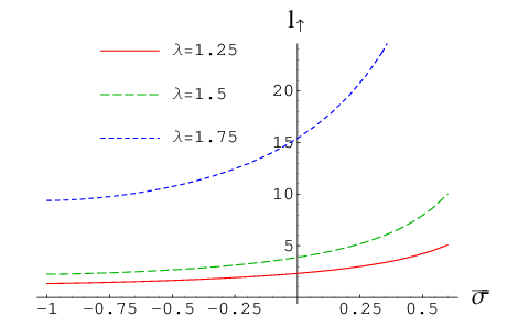
In figure 1, the size of the up spin domain ( $l_{\uparrow}$ ) is plotted at several values of $\lambda\in(1,2)$ as a function of $\bar{\sigma}$ . As $\lambda$ increases, the frustrating interaction becomes shorter ranged, and the size of the domains becomes larger as expected. One must be careful, however, in interpreting figure 1 since the unit itself depends on $\lambda$ . This exposes a difficulty of working with the continuum model with a variable exponent $\lambda$ , as the only length scale is dependent both on $\lambda$ and $J/Q$ . Figure 2 shows for fixed $\lambda=3/2$ the size of both spin domains, as well as their sum $L$ , as a function of the applied field $\mathrm{H}$ (obtained via Legendre transform).

Refer to caption — Figure 1: Size of the spin up domain in the ground state of (2) as a function of average spin $\bar{\sigma}$ . The vertical axis is in units of $\left(\frac{2-\lambda}{\lambda}\frac{J}{Q}\right)^{\frac{1}{2-\lambda}}$ .

III.3 Case III. $\lambda>2$

When $\lambda>2$ , to keep the energy density finite, the ultraviolet cutoff $a$ cannot be set to zero, and $a$ must be carried through the calculation. Although the analysis leading to (15) and (16) can be extended to $\lambda>2$ , the sum in (12) would diverge, and it is preferable to analyze the system entirely in real space, starting from (14). Only regions where $\sigma(r)\neq\sigma(r^{\prime})$ (i.e. $\sigma(r)\sigma(r^{\prime})=-1$ ) yield nonzero contributions in the second term, and after some algebra, for $L\gg a$ the energy density can be written as:

\epsilon(\bar{\sigma},L)=\frac{4J}{L}+\frac{4Q}{(\lambda-2)(\lambda-1)L}\left[\frac{C^{\prime}(\bar{\sigma},\lambda)+\alpha^{2-\lambda}}{L^{\lambda-2}}-\frac{1}{a^{\lambda-2}}\right]

(17)

where we have defined the following sum, convergent for $\lambda>1$ :

C^{\prime}(\bar{\sigma},\lambda)=\sum_{n=1}^{\infty}\left[(n+\alpha)^{2-\lambda}-2n^{2-\lambda}+(n-\alpha)^{2-\lambda}\right]~,

(18)

and $\alpha=(1+\bar{\sigma})/2$ . For larger $a/L$ there are corrections to $C^{\prime}$ of order $a/L$ . We set the derivative of the energy per site with respect to the period $L$ to zero and thus find the ground state $L$ :

$\displaystyle\frac{\mathrm{d}\epsilon}{\mathrm{d}L}$	$\displaystyle=$	$\displaystyle-\frac{4J}{L^{2}}-\frac{4Q}{(\lambda-2)L^{\lambda}}\left(C^{\prime}(\bar{\sigma},\lambda)+\alpha^{2-\lambda}\right)$
		$\displaystyle+\,\frac{4Q}{(\lambda-1)(\lambda-2)L^{2}}a^{2-\lambda}$
$\displaystyle 0$	$\displaystyle=$	$\displaystyle-J+\frac{Q}{\lambda-2}\left[\frac{a^{2-\lambda}}{\lambda-1}-L^{2-\lambda}\left(C^{\prime}(\bar{\sigma},\lambda)+\alpha^{2-\lambda}\right)\right]$
$\displaystyle\frac{J}{Q}$	$\displaystyle=$	$\displaystyle\frac{1}{\lambda-2}\left[\frac{a^{2-\lambda}}{\lambda-1}-\frac{\alpha^{2-\lambda}C^{\prime}(\bar{\sigma},\lambda)}{L^{\lambda-2}}\right]\,.$	(19)

In the present case of $\lambda>2$ , $C^{\prime}(\bar{\sigma},\lambda)>0$ , so the last line above will have a solution with finite L only below a critical value of $J/Q$ :

\displaystyle\left(\frac{J}{Q}\right)_{c}=\frac{a^{2-\lambda}}{(\lambda-2)(\lambda-1)}\,.

(20)

For larger values of $J/Q$ the energy is minimized by infinite $L$ so the ground state has macroscopic phase separation, since the energy of a domain wall is then always positive.

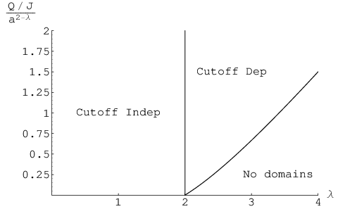
Thus, for $\lambda>2$ , this model with a given $J/Q$ may or may not show finite domains in its ground state, depending on the cutoff $a$ . In this regime, finite domains form in the ground state only for $J/Q<(J/Q)_{c}$ , as specified by (20). Above this value the ferromagnetic interaction is too strong relative to the antiferromagnetic interaction for domains to form. Figure 3 shows the regions of phase space where domains exist, and where the domain size is cutoff independent in the limit $a\rightarrow 0$ .

III.4 Case IV. $\lambda=2$

In the special case $\lambda=2$ , an analysis similar to the above $\lambda>2$ case can be done, which results in an energy density (valid for $L\gg a$ )

$\displaystyle\epsilon(\bar{\sigma},L)$	$\displaystyle=$	$\displaystyle\frac{4J}{L}+\frac{4Q\beta^{2}}{L}\left[\ln\left(\frac{a}{\alpha L}\right)-\frac{\alpha L}{a}\right]$	(21)
		$\displaystyle+\frac{4Q\alpha^{2}}{L}\left[\ln\left(\frac{a}{\beta L}\right)-\frac{\beta L}{a}\right]$
		$\displaystyle+\frac{8Q\alpha\beta}{L}\ln\left(\frac{a}{\alpha\beta L}\right)+\frac{F(\bar{\sigma})}{L}$

where $\beta=(1-\bar{\sigma})/2$ and $F(\bar{\sigma})$ is a function independent of $L$ . By solving $\frac{\mathrm{d}\epsilon}{\mathrm{d}L}=0$ we find that the ground state period $L_{0}$ is exponentially dependent on $J/Q$ with a prefactor proportional to $a$ :

L_{0}=a\exp\left[\frac{J}{Q}+F^{\prime}(\bar{\sigma})\right]

(22)

where $F^{\prime}(\bar{\sigma})$ is another function independent of $L$ and of order unity for $\bar{\sigma}\in[-1,+1]$ . This form can be argued from dimensional analysis, since $J/Q$ is dimensionless at $\lambda=2$ , and the only length scale in the problem is $a$ . The boundary case $\lambda=2$ separates the regime where $L$ approaches a finite limit given by (13) as $a\rightarrow 0$ for $\lambda<2$ , from the the cutoff-dependent regime for $\lambda>2$ .

IV Concluding Remarks

In summary, we have studied the generalized Coulomb-frustrated Ising model in a one dimensional continuum for different exponents $\lambda$ of the long range interaction ( $\lambda=1$ for the Coulomb case). We have derived an analytic solution for the ground state domain configuration of this model under the assumption that the ground state configuration has a simple periodic structure. This assumption has been confirmed by Monte Carlo simulations (see Appendix A). Such simulations can be done in any dimension $d$ , and mark an avenue for future work; more complicated domain patterns presumably do occur for $d>1$ .

We find that for $0<\lambda<2$ , as the magnetic field $\mathrm{H}$ is increased from $-\infty$ , the ground state is ferromagnetic until a critical field $-\mathrm{H}_{c}$ is reached, at which point isolated domains of flipped spins of finite length are formed in an otherwise polarized background. For $-\mathrm{H}_{c}\leq\mathrm{H}\leq\mathrm{H}_{c}$ , periodic configurations with $l_{\uparrow}$ up spins followed by $l_{\downarrow}$ down spins become the ground state, and the system is said to be in a “microemulsion” phase. In higher dimensions much numerical work has been done in the absence of a magnetic field(see LowEmery; ViotTarjus; MuMa), and applications have been made to magnetic thin filmsDeBellRMP in 2D, as well as the metal insulator transition in 2D and 3DOrtix2006. Analytical expressions analogous to our results can be derived assuming the ground state is simply periodic along only one directionNgVanderbilt. But more generally one is presumably forced to resort to approximations and numerics. The numerical Monte Carlo work, however, can be readily extended to higher dimensions, and can be used to investigate domain formation and behavior as a magnetic field is varied (i.e. in the non-charge-neutral case).

Our solutions describe how $l_{\uparrow}$ increases and $l_{\downarrow}$ decreases with increasing $\mathrm{H}$ . At zero field $l_{\uparrow}=l_{\downarrow}$ , and at $\mathrm{H}=\pm\mathrm{H}_{c}$ we find that $l_{\uparrow}$ or $l_{\downarrow}$ diverges to infinity, respectively, while the length of the “minority” domain remains nonzero and finite. For $\lambda\geq 2$ , whether or not the microemulsion phases appear in the transition between fully polarized up and down states depends on the dimensionless quantity $(Qa^{\lambda-2})/J$ . In the case that microemulsion phases do occur in this region, their properties depend on the ultraviolet cutoff $a$ . Our results provide more explicit examples of models with frustrating and sufficiently long range interactions that have ordered “microemulsion” phases instead of macroscopic phase separation. However, whether such a result is obtained in an inherently quantum system such as the 2D electron gas requires further investigation. In this context, it is worth noting that claims exist in the literature in favor of the classical scenario, both for the electron gasSpivak2004 and for the highly disordered Anderson model with long range Coulomb interactionsBhattRamakrishnan.

Appendix A Monte Carlo analysis

The approximation central to this paper is that the ground state of $\mathcal{H}_{\bar{\sigma}}$ (see eq. 2) has a simple periodic structure. While this has been proved for $\mathrm{H}=0$ (i.e. $\bar{\sigma}=0$ ), no such result exists for nonzero magnetization. Thus, to justify the approximation, we have performed Monte Carlo simulations on a discretized version of eq. 2:

\mathcal{H}_{\bar{\sigma}}=-J\sum_{i}\sigma_{i}\sigma_{i+1}+Q\sum_{ij}\frac{\sigma_{i}\sigma_{j}}{|i-j|^{\lambda}}~.

(23)

If we introduce a lattice spacing parameter $a$ , then in the limit $J/Q\rightarrow 0$ and $a\rightarrow 0$ such that $\frac{Qa^{\lambda-2}}{J}=C$ for constant $C$ , the above Hamiltonian is equivalent to the continuum formulation (eq. 2) with $J/Q=C$ . We solve for the ground state the discretized model using a Monte Carlo algorithm with simulated annealing. Updates are determined by a Wolff cluster methodGrousson2001 which preserves the overall magnetization, and thus $\bar{\sigma}$ is fixed during a simulation run (similar to the analytical calculation). Enough runs are averaged over so that the variation in the sizes of the resulting domains is negligible. Additionally, the system configuration converged upon by each Monte Carlo run is compared to the exactly periodic configuration and it is seen that the energy density of the exactly periodic configuration is always equal to or lower than the energy density of the Monte Carlo result. In summary, we find that at any $\bar{\sigma}\in[-1,1]$ , and for all values of $J/Q$ the ground state consists of uniform spin up domains of length $l_{\uparrow}$ interleaved with uniform spin down domains of length $l_{\downarrow}$ (but $l_{\uparrow}\neq l_{\downarrow}$ ). Detailed results will be provided elsewhereNielsenMonteCarlo.

References

(1) P. W. Anderson, G. Yuval and D. R. Hamann, Phys. Rev. B 1, 4464 (1970); J. Bhattacharjee, S. Chakravarty, J. L. Richardson and D. J. Scalapino, Phys. Rev. B 24, 3862 (1981).
(2) G. Kotliar, P. W. Anderson and D. L. Stein, Phys. Rev. B 27, 602 (1983).
(3) R. N. Bhatt and A. P. Young, J. Magn. and Magn. Mat. 54-57, 191 (1986).
(4) M. E. Fisher, S.-k. Ma and B. G. Nickel, Phys. Rev. Lett. 29, 917 (1972).
(5) U. Löw and V. J. Emery, K. Fabricius, and S. A. Kivelson, Phys. Rev. Lett. 72, 1918 (1994).
(6) P. Viot and G. Tarjus, EuroPhys. Lett. 44, 423 (1998)
(7) Yan Mu and Yu-qiang Ma, J. Chem. Phys. 117, 1686 (2002).
(8) Kwok-On Ng and David Vanderbilt, Phys. Rev. B 52, 2177 (1995)
(9) B. Spivak and S. A. Kivelson, Phys. Rev. B 70, 155114 (2004).
(10) R. Jamei, S. A. Kivelson, and B. Spivak, Phys. Rev. Lett. 94, 056805 (2005)
(11) J. Lorenzana, C. Castellani, and C. Di Castro, Phys. Rev. B 64, 235127 (2001)
(12) A. Giuliani, J. L. Lebowitz and E. H. Lieb, Phys. Rev. B 74, 064420 (2006).
(13) M. Grousson, G. Tarjus and P. Viot, Phys. Rev. E 62, 7781 (2000).
(14) K. De’Bell, A. B. MacIsaac, and J. P. Whitehead, Rev. Mod. Phys. 72, 225 (2000)
(15) C. Ortix, J. Lorenzana, and C. Di Castro, Phys. Rev. B 73, 245117 (2006)
(16) R. N. Bhatt and T. V. Ramakrishnan, J. Phys. C 17, L639 (1984) and R. N. Bhatt, Philos. Mag. B 50, 189 (1984) have extended the classical model of A .L. Efros and B. I. Shklovskii, J. Phys. C 8, L49 (1975) of electrons on highly disordered sites interacting with long range Coulomb interactions to include quantum mechanical hopping.
(17) M. Grousson, G. Tarjus and P. Viot, Phys. Rev. E 64, 36109 (2001).
(18) Erik Nielsen, R. N. Bhatt, and D. A. Huse, in preparation.