Correspondence between Andreev reflection and Klein tunneling in bipolar graphene

Tunneling through an n-p junction in graphene is called Klein tunneling Kat06; Che06; Che07 with reference to relativistic quantum mechanics, where it represents the tunneling of a particle into the Dirac sea of antiparticles Kle29. Klein tunneling in graphene (see Fig. 1) is the tunneling of an electron from the conduction band into hole states from the valence band — which plays the role of the Dirac sea. Several recent experiments Hua07; Wil07; Ozy07 have investigated this unusual coupling of electron-like and hole-like dynamics.

In the course of an analysis of these experiments a curious similarity was noticed Two07 between negative refraction Che07; Not00 at an n-p junction and Andreev retroreflection And64 at the interface between a normal metal (N) and a superconductor (S). As illustrated in Fig. 2a,b, the trajectories at an n-p junction and at an NS junction are related by mirroring $x\mapsto-x$ at the interface (taken at $x=0$). Here we show that the similarity is not limited to classical trajectories, but extends to the fully quantum mechanical wave functions and energy spectra. This implies that quantum effects associated with superconductivity, such as the proximity effect and the Josephson effect, have analogues in an n-p junction.

We have found a precise mapping between the Dirac Hamiltonian DiV84 of an n-p junction and the Dirac-Bogoliubov-De Gennes Hamiltonian Bee06 of an NS junction under the condition that the electrostatic potential $U$ in the n-p junction is antisymmetric, $U(-x,y)=-U(x,y)$, with respect to the interface. The Fermi level is chosen at zero energy, symmetrically between the n and p regions. Such a symmetric n-p junction turns out to have the same excitation spectrum as an NS junction for excitation energies $\varepsilon$ small compared to the superconducting gap $\Delta$. After presenting the mapping in its mathematical form, we consider the two major physical implications: Zero density of states at the Fermi level and persistent current flow in equilibrium. A comparison with computer simulations of a tight-binding model of graphene is presented at the end of the paper.

Derivation of the mapping. — The correspondence between Klein tunneling and Andreev reflection consists of a mapping of an eigenstate $\Psi$ of the Dirac Hamiltonian $H$ of a symmetric n-p junction onto electron and hole eigenstates $\Psi_{e}$ and $\Psi_{h}$ in the normal part $x>0$ of the NS junction. The Dirac Hamiltonian is given (in the valley-isotropic representation) by

with $\bm{p}=-i\hbar(\partial/\partial x,\partial/\partial y)$ the momentum operator in the $x-y$ plane of the graphene layer, $\bm{A}=Bx\bm{\hat{y}}$ the vector potential of a perpendicular magnetic field $B$, and $v$ the electron velocity. The Pauli matrices $\sigma_{i}$ and $\tau_{i}$ act, respectively, on the sublattice and valley degree of freedom (with $\sigma_{0}$ and $\tau_{0}$ a $2\times 2$ unit matrix). We introduce the time-reversal operator ${\cal T}=-(\sigma_{y}\otimes\tau_{y}){\cal C}$, with ${\cal C}$ the operator of complex conjugation, and the parity operator ${\cal P}=i(\sigma_{x}\otimes\tau_{0}){\cal R}$, with ${\cal R}$ the operator of reflection ($x\mapsto-x$). The key property of the Dirac Hamiltonian that we need, in order to map the symmetric n-p junction onto an NS junction, is the anticommutation relation

satisfied for any $B$ when $U(-x,y)=-U(x,y)$.

Starting from a solution $H\Psi=\varepsilon\Psi$ of the Dirac equation in the n-p junction we now construct an eigenstate in the NS junction at the same eigenvalue $\varepsilon$ by means of the transformation

According to Refs. Bee06; Tit06 the electron and hole wave functions $\Psi_{e},\Psi_{h}$ in the normal part of the NS junction should satisfy

with a boundary condition at the NS interface that for $|\varepsilon|\ll\Delta$ takes the form

The proof of the mapping now follows by inspection: Firstly, Eq. (4) results directly from the transformation (3) with the anticommutation relation (2). Secondly, since $\Psi$ is continuous at $x=0$, the boundary condition (5) is automatically satisfied.

The applicability of the mapping extends to the crystallographic edges of the graphene layer in the following way: The edges of the n-p junction are described by the boundary condition $\Psi(\bm{r})=M(\bm{r})\Psi(\bm{r})$ for $\bm{r}$ at the edge McC04; Akh07. The mapping to an NS junction still holds, provided that $M$ commutes with ${\cal P}$, which requires

For example, an armchair edge parallel to the $x$-axis (with $M\propto\sigma_{x}$ independent of $x$) satisfies the requirement (6), but a zigzag edge parallel to the $x$-axis ($M\propto\sigma_{z}$) does not. A pair of zigzag edges at $x=\pm W$ [with $M(\pm W,y)=\pm\sigma_{z}\otimes\tau_{z}$], on the other hand, do satisfy the requirement (6). An infinite mass boundary condition [with $M(\pm W,y)=\pm\sigma_{y}\otimes\tau_{z}$], likewise, satisfies this requirement.

Suppression of the density of states. — We have calculated the density of states $\rho(\varepsilon)$ by solving the Dirac equation in the n-p junction of Fig. 2a. The Fermi level (taken at $\varepsilon=0$) is separated from the Dirac point by the energy $\pm\mu$ in the n and p regions. We take an abrupt interface (width $d$ small compared to the Fermi wave length $\lambda_{F}=hv/\mu$) and wide and long n and p regions (width $W\gg\lambda_{F}$, length $L\gg W$). The precise choice of boundary condition at $x=\pm W$ does not matter in this regime, as long as it preserves the symmetry of the geometry.

The calculation for the bipolar junction follows step-by-step the analogous calculation for the Josephson junction in Ref. Tit07. The dispersion relation (smoothed over rapid oscillations) is given by

with $m=0,\pm 1,\pm 2,\ldots$ the mode index and $\hbar q$ the momentum parallel to the n-p interface. (The energy $E_{T}=\hbar v/2W$ is the Thouless energy, which is $\ll\mu$ for $W\gg\lambda_{F}$.) The resulting density of states $\rho(\varepsilon)=(4/\pi)\sum_{m}|\partial\varepsilon_{m}/\partial q|^{-1}$ is plotted in Fig. 3. It vanishes linearly as

for small $|\varepsilon|$, with $\rho_{0}=(2\mu/\pi)(\hbar v)^{-2}$ the density of states (per unit area and including spin plus valley degeneracies) in the separate n and p regions. This suppression of the density of states at the Fermi level by a factor $\varepsilon/E_{T}$ is precisely analogous to an NS junction, where the density of states is suppressed by the superconducting proximity effect (compare, for example, our Fig. 3 with Fig. 8 of Ref. Tit07). In particular, the peaks in $\rho(\varepsilon)$ at $\varepsilon=\pi E_{T}(m+\tfrac{1}{2})$ are analogous to the De Gennes-Saint James resonances in Josephson junctions DeG63.

In a semiclassical description, the suppression of the density of states in the n-p junction can be understood as destructive interference of the electron-like and hole-like segments of a periodic orbit (solid and dashed lines in Fig. 2a). At the Fermi level, the dynamical phase shift accumulated in the n and p regions cancels, and what remains is a Berry phase shift of $\pi$ from the rotation of the pseudospin of a Dirac fermion Nov05; Zha05.

Persistent current. — If the n and p regions enclose a magnetic flux $\Phi$, as in the ring geometry of Fig. 4 (inset), then the Berry phase shift can be compensated and the suppression of the density of states can be eliminated. The resulting flux dependence of the ground state energy $E={\cal A}\int_{-\infty}^{0}\rho(\varepsilon)\varepsilon\,d\varepsilon$ (with ${\cal A}$ the joint area of the n and p regions) implies that a current $I=dE/d\Phi$ will flow through the ring in equilibrium at zero temperature, as in a Josephson junction Imr97. According to Eq. (8), the order of magnitude

of this persistent current is set by the level spacing $\delta=({\cal A}\rho_{0})^{-1}$ and by the Thouless energy $E_{T}=\hbar v/\pi r=N\delta$ in the ring geometry (of radius $r$ and width $w\ll r$, supporting $N=4\mu w/\pi\hbar v\gg 1$ propagating modes). Because of the macroscopic suppression of the density of states, this is a macroscopic current — larger by a factor $N$ than the mesoscopic persistent current in a ballistic metal ring Imr97; But83.

We have calculated $I(\Phi)$ for a simple model of an abrupt n-p junction in an $N$-mode ring without intermode scattering, neglecting the effect of the curvature of the ring on the spectrum and also assuming that the magnetic field is confined to the interior of the ring. (These approximations are reasonable for $\lambda_{F}\ll w\ll r$.) The slowly converging, oscillatory integral over $\rho(\varepsilon)$ was converted into a rapidly decaying sum over Matsubara frequencies by the method of Ref. Bro97. The zero-temperature result is plotted in Fig. 4 (solid curve). The maximal persistent current is $I_{c}\approx 0.2\,I_{0}$. This is the same value, up to a numerical coefficient, as the critical current of a ballistic Josephson junction note1. We have also included the results at finite temperature, showing the decay when the thermal energy $k_{B}T\simeq E_{T}$.

Comparison with computer simulations. — To test our analytical predictions, we have performed computer simulations of a tight-binding Hamiltonian on a honeycomb lattice (lattice constant $a$). We took a symmetric n-p junction with zigzag boundaries at $x=\pm W$ (with $W/a=400$) and calculated the density of states $\rho(\varepsilon)$, smoothed by a Lorentzian (width $0.01\,E_{T}$) to eliminate the rapid oscillations. Results are shown in Fig. 5, for different Fermi wave lengths $\lambda_{F}=hv/\mu$ and widths $d$ of the n-p interface [potential profile $U(x)=-\mu\tanh(4x/d)$]. A clear suppression of $\rho(\varepsilon)$ is observed within an energy range $E_{T}$ from the Fermi level at $\varepsilon=0$. The suppression is somewhat smaller than predicted by Eq. (8) (black solid line), in particular for $d\simeq a$ (red curve, when the Dirac equation no longer applies) and for $d\gtrsim\lambda_{F}$ (blue curve, when Klein tunneling happens only near normal incidence Che06).

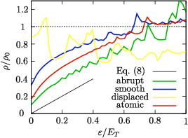
As expected, the suppression is sensitive to perturbations of the reflection symmetry. For example, as shown in Fig. 5 (yellow curve), a displacement of the n-p interface by $\lambda_{F}$ spoils the systematic destructive interference due to the Berry phase, and thus eliminates the suppression of the global density of states.

We would still expect an effect on the local density of states if we could confine the carriers to the n-p interface. This might be achieved by means of the saddle point potential $U=\mu\,{\rm sign}\,(xy)$ of Fig. 2c, or by means of the nonuniform magnetic field $B=B_{0}x$ of Fig. 2d. Destructive interference of the periodic orbits in each of these unbounded geometries will suppress the local density of states near the interface by the same mechanism as in the confined geometry of Fig. 2a. Because of disorder, the suppression will be limited to a mean free path or corrugation length from the n-p interface. Since the predicted suppression of the density of states at the Fermi level happens at a large energy separation $\mu$ from the Dirac point (see Fig. 1), it should be distinguishable in a local measurement (for example, by a tunneling probe) from any features associated with the conical singularity in the band structure at the Dirac point.

From a different perspective, the correspondence derived here offers the intriguing opportunity to observe superconducting analogies in non-electronic systems governed by the same Dirac equation as graphene. An example would be a two-dimensional photonic crystal on a honeycomb or triangular lattice Rag06; Sep07, in which the analogue of an n-p junction has been proposed recently Gar07. The detrimental effects of disorder should be relatively easy to avoid in such a metamaterial.

We acknowledge discussions with J. Nilsson and R. A. Sepkhanov. This research was supported by the Dutch Science Foundation NWO/FOM.

References

- (1) M. I. Katsnelson, K. S. Novoselov, and A. K. Geim, Nature Phys. 2, 620 (2006).
- (2) V. V. Cheianov and V. I. Fal’ko, Phys. Rev. B 74, 041403(R) (2006).
- (3) V. V. Cheianov, V. I. Fal’ko, and B. L. Altshuler, Science 315, 1252 (2007).
- (4) O. Klein, Z. Phys. 53, 157 (1929).
- (5) B. Huard, J. A. Sulpizio, N. Stander, K. Todd, B. Yang, and D. Goldhaber-Gordon, Phys. Rev. Lett. 98, 236803 (2007).
- (6) J. R. Williams, L. DiCarlo, and C. M. Marcus, Science 317, 638 (2007).
- (7) B. Özyilmaz, P. Jarillo-Herrero, D. Efetov, D. A. Abanin, L. S. Levitov, and P. Kim, Phys. Rev. Lett. 99, 166804 (2007).
- (8) J. Tworzydło, I. Snyman, A. R. Akhmerov, and C. W. J. Beenakker, Phys. Rev. B 76, 035411 (2007).
- (9) M. Notomi, Phys. Rev. B 62, 10696 (2000).
- (10) A. F. Andreev, Sov. Phys. JETP 19, 1228 (1964).
- (11) D. P. DiVincenzo and E. J. Mele, Phys. Rev. B 29, 1685 (1984).
- (12) C. W. J. Beenakker, Phys. Rev. Lett. 97, 067007 (2006).
- (13) M. Titov and C. W. J. Beenakker, Phys. Rev. B 74, 041401(R) (2006).
- (14) E. McCann and V. I. Fal’ko, J. Phys. Condens. Matter 16, 2371 (2004).
- (15) A. R. Akhmerov and C. W. J. Beenakker, Phys. Rev. Lett. 98, 157003 (2007).
- (16) M. Titov, A. Ossipov, and C. W. J. Beenakker, Phys. Rev. B 75, 045417 (2007).
- (17) P. G. de Gennes and D. Saint-James, Phys. Lett. 4, 151 (1963).
- (18) K. S. Novoselov, A. K. Geim, S. V. Morozov, D. Jiang, M. I. Katsnelson, I. V. Grigorieva, S. V. Dubonos, and A. A. Firsov, Nature 438, 197 (2005).
- (19) Y. Zhang, Y.-W. Tan, H. L. Stormer, and P. Kim, Nature 438, 201 (2005).
- (20) Y. Imry, Introduction to Mesoscopic Physics (Oxford University Press, Oxford, 1997).
- (21) M. Büttiker, Y. Imry, and R. Landauer, Phys. Lett. A 96, 365 (1983).
- (22) P. W. Brouwer and C. W. J. Beenakker, Chaos, Solitons & Fractals 8, 1249 (1997); online at cond-mat/9611162.
- (23) The finite-temperature calculation of is worked out in the Appendix, and compared with the analogous result in a Josephson junction.
- (24) S. Raghu and F. D. M. Haldane, cond-mat/0602501.
- (25) R. A. Sepkhanov, Ya. B. Bazaliy, and C. W. J. Beenakker, Phys. Rev. A 75, 063813 (2007).
- (26) J. L. Garcia-Pomar, A. Cortijo, and M. Nieto-Vesperinas, arXiv:0710.1004.
- (27) C. W. J. Beenakker and H. van Houten, in: Nanostructures and Mesoscopic Systems, edited by W. P. Kirk and M. A. Reed (Academic, New York, 1992); online at cond-mat/0512610.
- (28) C. Ishii, Prog. Theor. Phys. 44, 1525 (1970).
- (29) J. Bardeen and J. L. Johnson, Phys. Rev. B 5, 72 (1972).
- (30) A. V. Svidzinsky, T. N. Antsygina, and E. N. Bratus, Sov. Phys. JETP 34, 860 (1972); J. Low Temp. Phys. 10, 131 (1973).
- (31) M. Büttiker and T. M. Klapwijk, Phys. Rev. B 33, 5114 (1986).