Rough Isometries of Lipschitz Function Spaces
Abstract
We show that rough isometries between metric spaces can be lifted to the spaces of real valued 1-Lipschitz functions over and with supremum metric and apply this to their scaling limits. For the inverse, we show how rough isometries between and can be reconstructed from structurally enriched rough isometries between their Lipschitz function spaces.
1 Introduction
Is there a qualitative difference between functions on a continuum and functions on a discrete set , which is -dense in ? Obviously, singularities may emerge on . But, apart from that, are there more differences? In this paper we want to show that, when we are concerned with 1-Lipschitz functions, nothing new is added in the passage from discrete to continuum. Even more, the coarse geometry of a metric space (in the sense of its rough isometries) is already determined by its 1-Lipschitz function space.
There are detailed books and lots of articles on many aspects of Lipschitz function spaces, including isometries between them. A nice survey is Weaver’s book on Lipschitz Algebras [W] (cf. section 2.6, where Weaver elaborates on the exact same questions we want to tackle here, but in a non-coarse context and under different conditions). However, to the knowledge of the author, no book nor paper dealt with their coarse geometry yet. On the other hand, Lipschitz functions naturally appear in many aspects of coarse geometry, like the Levy concentration phenomenon or the definition of Lipschitz-Hausdorff distance in [G2]. But they are not dealt with as metric spaces either.
The two main theorems we want to show are as following:
Theorem 1
Let be (possibly infinite) metric spaces, . For each -isometry , there is a -ml-isomorphism such that is -near for all .
Theorem 2
Let be complete (possibly infinite) metric spaces and . For each -ml-isomorphism there is a -isometry , such that is -near for all .
The theorems above can be seen as variants on two 60 year old theorems. The first is given by Hyers and Ulam in [HU]:
Theorem 3 (Hyers-Ulam)
Let by compact metric spaces and let and be the spaces of all real valued continuous functions on and , respectively. If is a homomorphism of onto which is also an -isometry, then there exists an isometric transformation of onto such that for all in . Corollary: The underlying metric spaces and are homeomorphic.
As we make use of the order-lattice structure of the Lipschitz function spaces in our proofs, the following theorem by Kaplansky [Kp] is related to our results as well, we state it in its formulation by Birkhoff ([B], 2nd ed. p. 175f.):
Theorem 4 (Kaplansky)
Any compact Hausdorff space is (up to homeomorphism) determined by the lattice of its continuous functions.
The structure of this paper is as follows: In the first section we want to recall the notions of rough isometry, lattices, and Lipschitz functions, and our notation for metrics with infinity. In the second section we will proof some simple properties of Lipschitz function spaces and define what we call “-functions”. In the third and fourth section, we will proof the two main theorems of this paper. The fifth section presents an application in the context of scaling limits, giving a partial answer to the introductory question. The final section provides some conclusions and perspectives for future development of this subject.
1.1 Notation
Throughout this paper, let and be (possibly infinite) metric spaces in the following sense:
Definition 5
A (possibly infinite) metric space is a non-empty set together with a mapping which is positive-definite and fulfills the triangle-inequality. For this, we set and for all and call positive iff . is called true metric space iff for all .
We will make heavy use of the symbol
for some in or and . To make sense of this in case one of the distances becomes infinite, we define the former symbol to be equivalent to
| and |
In particular, we find . This might seem unfamiliar. Note however, that can be perfectly understood as a (possibly infinite) metric on itself. (Note that there is no non-trivial convergence to in this metric, is just an infinitely far away point.)
In most cases we call metrics on and both “” as it should be clear from the elements which metric is meant.
Furthermore, it’s obvious that a (possibly infinite) metric space always is a disjoint union of true metric spaces with iff with , . We call the components of . We call complete, iff all of its components are complete as true metric spaces.
Definition 6
Two (set theoretic) mappings are -near to each other, , iff . (We drop brackets where feasible.)
A (set theoretic) mapping is -surjective, , iff for each there is s.t. .
Definition 7
A (not neccessarily continuous) map is called an -isometric embedding, (which shall always imply ), iff
for all .
A pair , of -isometric embeddings is called an -isometry (or rough isometry) iff and are -near the identities on and , respectively. When we speak of an “-isometry ” a corresponding map shall always be implied.
and are called -isometric, iff there is an -isometry between them.
It’s difficult to attribute the concept of rough isometry to a single person, as it was always present in the notion of quasi-isometry, which itself was an obvious generalization of what was then called pseudo-isometry by Mostow in his 1973-paper about rigidity (see [M], [G1], [Kn]). Recent developments about the stability of rough isometries can be found in [Ra].
Definition 8
A mapping is called -Lipschitz (i.e. “-Lipschitz map on -scale” in [G3]), , iff
If , is -Lipschitz (continuous). Define to be the set of all -Lipschitz functions , and , .
If nothing else is said, is the default target space for a Lipschitz function.
Assume to be a -Lipschitz function on and for some . Then clearly for all in finite distance to . Thus, if is a true metric space, we have .
Definition 9
A lattice is a set together with two mappings which are commutative, associative and fulfill the absorption laws for all . A lattice is called complete iff all infima and all suprema of all subsets of exist in .
Of particular interest is with and pointwise minimum and maximum respectively, and , pointwise infimum and supremum. The following proposition is a special case of Lemma 6.3 in [H] and Proposition 1.5.5 in [W]. To keep this article self-contained, we nevertheless give a proof:
Proposition 10
Let be a (possibly infinite) metric space. Then is complete as a lattice.
Proof Let , be in . Obviously, is complete as a lattice, with and . So we define pointwise
and observe that and are Lipschitz: Let be arbitrary. Then holds
for all , and thus, by passing to the infimum:
Same for .
Example 11
The space of real-valued continuous functions is not a complete lattice with pointwise minimum and maximum: Choose , , the infimum is not continuous. The same example shows that the space of all Lipschitz-functions with arbitrary Lipschitz constant is no complete lattice.
On , we consider the (possibly infinite) supremum metric
Note that is no metric lattice in the sense of Birkhoff [B]: There is no valuation on inducing , and property (4) of Theorem 1, p. 230 (third edition) is explicitly violated even by bounded Lipschitz functions.
2 Fundamental properties
Proposition 12
For arbitrary set theoretic functions , , some arbitrary index set, holds:
Proof For , both inequalities are trivial. Assume . As and commute, it suffices to show
for any .
First we handle infinities. First inequality: Assume there is with . We can ignore all such ’s from , unless all and are . In this case on both sides are zeros. Now assume . Then appears on the right side and trivializes the inequality. So we can restrict to finite and . Note that can only happen when all .
Second inequality: Assume , but is finite. Then there is an upper bound for but not for . Hence the right side becomes infinite, too. Note that infinite or automatically lead to infinite or , respectively.
Without restriction let , and let . Let be arbitrary. Then there is an with . Furthermore we have , hence . Altogether:
Now let .
The other inequality works the same way.
Next we define a special version of rough isometry, suiting the lattice structure of Lipschitz function spaces. The main new property will be an “approximate lattice homomorphism”. It exists in various versions, as Thomas Schick pointed out to us:
Proposition 13
Let be (possibly infinite) metric spaces and an -isometric embedding, . Then the following properties are equivalent:
- 1.
for all
- 2.
for all
- 3.
For all , , some index set, holds:
and
Proof (3) (2): .
(2) (1): Assume there is some such that . From follows , thus , in particular , contradiction.
(1) (3): Obviously for all , hence . We calculate the supremum over all : . On the other hand, for every there is some with . As is an -isometric embedding, this yields , hence
Let . The other approximation works analogously.
We extend property (3) from Proposition 13 to allow , and use it to define the notion of ml-isomorphisms:
Definition 14
Let be (possibly infinite) metric spaces. An -ml-homomorphism, is an -isometric embedding , with
| and |
for all , , some index set.
An -ml-isomorphism is a pair of -ml-homomorphisms and , s.t. and are -near their corresponding identities. When we speak of an “-ml-isomorphism ”, the corresponding shall always be implied.
Proposition 15
For any -ml-isomorphism holds .
Proof As Andreas Thom pointed out, this follows directly from Definition 14 when . There’s also a -proof avoiding empty index sets: Let be an -ml-isomorphism. We certainly know , hence
Now apply Proposition 12 to see
and use .
Proposition 16
A -surjective -ml-homomorphism induces a -ml-isomorphism .
Proof For each choose an element , s.t. . We show that the pair defines a -ml-isomorphism. The first inequality in Definition 14 is standard in coarse geometry:
for all . We now show that fulfills the second and third inequality as well. Both can be handled the same way:
Here we used (i) is -isometric embedding, (ii) is near identity, (iii) is ml-homomorphism, (iv) Proposition 12, (v) is near identity.
Finally we show that is -near identity:
is no algebra, like e.g. . Thus we can’t give a basis of functions and reconstruct by linear combinations. However, we can use the lattice structure to give another kind of “basis” for : Minimal Lipschitz functions with a given value at a single point.
Definition 17
Let and be arbitrary. Define by .
Note that this definition applies to or as well: If , we have , and if :
-functions with will be called infinite, else finite. Infinite -functions are infinitely high characteristic functions for ’s components.
Proposition 18
Let , . Then holds:
Proof Note that if the first and second case coincide, as . Assume without restriction . Let
Let’s start with infinite cases. If , we get on both sides. If , , we get . This is correct, as in this case the -functions are equal. If , we get again, for each variant of . If but , the two -functions have different components as support, and thus becomes the maximum of the differences, this is .
Now we assume . First case: . Then we have
In addition, we have , , thus . Hence . Second case: .
And:
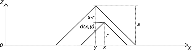
Corollary 19
For all holds:
Proof
Follows directly from Proposition 18.
This Corollary points us at an interesting aspect of -functions: When we analyse the metric space with metric for a fixed , we find it naturally isometric to with the cut-off-metric for all . Only in the limit , will restore the full metric of . Ironically, obviously cuts away the coarse, large-scale information of (in which we’re primarily interested) and conserves the topological, small-scale informations. The large-scale information of is still present, but more subtle to access.
Proposition 20
For all holds: , where the latter is a pointwise maximum, not only supremum. If is complete, the set is (topologically) closed.
Proof Let . Clearly, we have , as . We now observe that
For , this is clear. For , this follows from Lipschitz continuity ().
Furthermore, we notice that we deal with pointwise maxima: Each supremum of is taken by .
Let be any sequence converging to , , . First we notice
hence . Assume and finite. Then there is with and must have a lower bound for large enough . By Cauchy criterion there is such that for all we have
Due to Proposition 18 we conclude that for large enough
Thus as well as are Cauchy-sequences. As and are metrically complete, we find . As is continuous, we have , and . Now we only have to show . But this is clear, as for large enough we have
Now assume to be infinite (i.e. ). Then
has to be infinite as well for large enough (there is no
non-trivial convergence to infinity in the chosen metric on ) and
Proposition 18 shows for
large enough . Hence .
We make some more use of the black magic of Proposition 12:
Proposition 21
For all -isometries and holds:
Proof We observe that can be rewritten to
where : Each element of (respectively ) appears at least once in , and multiple instances don’t matter, as is idempotent. Now Proposition 12 yields:
Let . Case 1: . Then
Case 2: :
3 Inducing rough ml-isomorphisms
We make a first use of the notions of the preceding section. We proof that each -isometry lifts to an -isometry . Even better, is an -ml-isomorphism, and is near .
The next lemma is kind of a smoothening theorem. It states that the space of -Lipschitz functions over is -dense in the space of -Lipschitz functions over for all . A similar result for continuous functions is given by Petersen in [P], section 4.
Lemma 22
Let . Define
Then and are -near.
Proof We observe that is never larger than for all . So we have
and furthermore
As and we
conclude the statement. (Note that each negative value is surpassed by at
least one non-negative value, i.e. never occurs after taking the
supremum.)
Proposition 23
If is an -isometry, and any mapping which is -near , then is a -ml-isomorphism.
Proof (i) We show for all . We have
As next we notice . Now let be arbitrary, such that . Then as is 1-Lipschitz. Hence
(ii) For we observe that and , as well as and . Hence, assume . We know
as the infimum is calculated pointwise. Hence, with Proposition 12:
Same for supremum.
Theorem 24 ( Th. 1)
Given an -isometry , defines a -ml-isomorphism from to .
Proof Let be arbitrary. satisfies
Hence, and are -near (Lemma 22). However, is in , as it is a supremum of Lipschitz functions. Thus we can apply Proposition 23 to . Same holds for (Definition 7). It remains to show that and are near their respective identities.
We already saw that is -near
. Similarly is -near
and thus is -near
. Finally, is -near identity,
and as is 1-Lipschitz, is -near ,
too. All this adds up to . Same for .
4 Inducing rough isometries
In this section, we show the reversal of Theorem 24: Given an -ml-isomorphism we construct a rough isometry such that is near .
Recall the definition of a join-irreducible:
It is interesting to see that the finite -functions defined in Definition 17 satisfy a much more powerful version of join-irreducibility:
Lemma 25
Let , complete. The following are equivalent:
- 1.
is a finite -function, i.e. ,
- 2.
Proof In (2), the case is trivial. Hence, assume to be finite.
(1)(2): Let and be s.t. holds. Choose arbitrary and , , . As
there has to be a such that , otherwise would be a smaller upper bound for all then . From this, we see
Case 1: . Then we have , and
Case 2: . Then and
holds trivially.
On the other hand, we have
and thus .
(2)(1): Choose , , , . This yields a sequence of indizes (= points in ) such that . As is closed, we have either for some , or for any . Now assume . Then
This is a contradiction to Proposition 18, hence
is a finite -function.

Example 26
Lemma 25 does not hold for , just insert .
Recalling the short note after Corollary 19, the metric information of is encoded in the -functions and the distances between them. However, these functions are at first sight just some arbitrary subset of and thus there’s no hope for the metric space to hold the full information about ’s metric. The preceding Lemma now explains to us, that the (finite) -functions are not arbitrary at all – they have a specific, lattice theoretic property that distinguishes them from the remaining functions. Hence, in some sense the metric information of is now part of the combined metric and lattice structure of .
Proposition 27
Let be complete. Then the set of all -functions in is topologically closed. In addition, the set of all finite -functions is topologically closed.
Proof Let be some sequence of -elements in with limit . If there is a subsequence with for , then this subsequence and hence converges to for any . So assume is positive for large enough . Due to Proposition 18 we have:
As the left side becomes arbitrarily small, whereas
has a positive lower limit, only the second and third
case may occur for . For large enough ,
these cases don’t mix anymore. The third case is trivial. From the
second case we conclude and , and thus and . Clearly, . In particular, is finite in this
case, which proofs the second statement of the Proposition.
Lemma 28
Let , be complete, and an -ml-isomorphism. Then maps finite -functions -near finite -functions.
Proof Let be some finite -function. Represent via -functions , . Let be arbitrary. Then we have
Applying Lemma 25 to , we know that there exists such that
must be a finite -function, as
Case 1: . Choose .
Case 2: . The preceding argument yields a sequence of finite
-functions converging to . As of Proposition
27, must be a finite -function as
well.
The preceding Lemma is the critical point in our analysis: We can use -functions as building blocks for Lipschitz functions, as Proposition 20 tells us. From Lemma 28 we now know that these building blocks (or, at least, the finite versions) behave sensible under -ml-isomorphisms , such that we only have to understand how they are mapped by to reconstruct all other Lipschitz functions. In particular, as they are strongly connected to the underlying spaces, they allow us to define mappings between them:
Lemma 29
Let be complete, . Let be an -ml-isomorphism, . Then there is a map such that
for all , . For , we may replace “” by “”.
Proof In the following proof, the first two cases will deal with and finite , the third with and finite and the fourth with .
Case 1 and 2: For each , choose and such that is -near (use Lemma 28).
Case 1: , . Let be -near . Then by Proposition 15 holds
In the same way, we have
We now take a look at
Now we calculate by hand. From Proposition 18, could be or . We know
hence . But, as , but , can’t be (here we use ). Remains
As shown above, , hence
This, and , yield

Case 2: , . Obviously,
As and (see above), we receive and . This adds up to .
Case 3: , . As of Lemma 28, for all we can choose such that for some . From Proposition 15 we see , hence . Now, let be arbitrary. Let , such that . Clearly, from the distance to 0 we again have . From
we conclude
Due to Proposition 18 this can happen iff (a) or (b) or (c) . Case (c) prooves our statement, case (b) can’t happen: iff , which contradicts . So, assume case (a). Then , which contradicts , or . But the case is trivial, as we already saw from Proposition 15 that
Case 4: . We know . Using our result for finite , we conclude
Apply to see that is
-near .
Lemma 30
as defined in the proof of Lemma 29 is a -isometry.
Proof From Corollary 19 follows
Applying Lemma 29 for large enough yields:
And of course:
Hence
i.e. is a rough isometric embedding. Just as was constructed from , we construct from . It remains to show that and are near identities. Again, we make use of Corollary 19:
Same for .
Theorem 31 ( Th. 2)
Let be complete (possibly infinite) metric spaces and . For each -ml-isomorphism there is a -isometry , such that is -near .
5 Scaling limits
Definition 32
Let the rough distance between two (possibly infinite) metric spaces and be the infimum over all such that and are -isometric, or if there are none. If , the spaces and will be called pseudo-isometric.
The rough distance fulfills triangle-inequality, as concatenation of an - and a -isometry is an -isometry. It is closely related to the Gromov-Hausdorff-Distance for compact spaces, but may differ in a variable between and (i.e., they are Lipschitz-equivalent, see e.g. [G2], Proposition 3.5).
Pseudo-isometry is a little bit less than isometry. However, they are equivalent if only compact spaces are compared (e.g. [P], [G2]), or if we deal with simple graphs, due to their integer metric. A nice article about scaling limits, Gromov-Hausdorff distances and quasi-isometries in the case of graphs and Cayley graphs is [Re].
Definition 33
Let be the non-small groupoid of all pseudo-isometry-classes of metric spaces with -isometries as morphisms. is a (possibly infinite) metric on in a natural way.
Each of the components of can be endowed with a metric and topology, with the only drawback of being proper classes. This “topology” allows us to define the convergence of metric spaces to another metric space, up to pseudo-isometry. is complete in this “topology” (cf. [P], Proposition 6, the proof works in non-compact and non-separable cases as well).
Definition 34
Let , and given by
which scales each metric space in by the factor (). This operation clearly is compatible with pseudo-isometry. Let be a space in . If the limit
exists for all sequences , then (resp. all members of ) is called the (strong) scaling limit of .
We now want to apply Theorem 24.
Corollary 35
Let be some (possibly infinite) metric spaces, such that is a strong scaling limit of ( is unique up to pseudo-isometry). Then there is a strong scaling limit of , and it is pseudo-isometric to . (“The scaling limit of the Lipschitz space is the Lipschitz space of the scaling limit.”)
Proof
As for , there are
-isometries with
.
These induce -ml-isomorphisms
, which are in
particular -isometries. Hence, . Proper rescaling of the associated Lipschitz functions further
shows is naturally isometric to , hence up to pseudo-isometry.
Note that we can restrict to a set of when calculating a scaling limit. Thus, we can make use of Banach’s fixed point theorem if restricts to a true metric on this set.
6 Perspectives
6.1 Generalizations
There are several obvious ways to generalize the two main theorems: Changing the target space or the metric on would break the main points of the proof, however single ideas might survive. The use of other types of functions is a similarly difficult question:
Example 36
Take and the inclusion, . The metric spaces of -valued continuous functions and with sup-norm are isomorphic to and respectively, which are not roughly isometric.
Another point is the inclusion of quasi-isometries. Although many ideas still work in the context of quasi-isometries, a function’s Lipschitz constant is distorted in the process of Lemma 22. Hence there happens to be a “mixing” of the Lipschitz function spaces , which creates deep problems and at the same time great potential: If we find a workable solution to this problem, a new class of function spaces for groups would emerge, “quasi-Lipschitz functions”, so to speak.
Another very promising approach is to explore the rough isometries of Hajłasz-Sobolev spaces ([H], chapter 5). These are subsets of function spaces, with a norm similar to the Sobolev norm. This norm contains a version of derivative which might compensate the obstruction we encounter with functions of arbitrary Lipschitz constant, at least for .
6.2 Category Interpretation
Let be (possibly infinite) metric spaces. We define
is well-defined as iff and because each pseudo-isometry-class contains a complete metric space. is a non-small groupoid with ml-isomorphisms as morphisms. In these terms, the mapping is a Lipschitz equivalence between the metric categories and , and a contravariant functor up to nearness of rough isometries.
6.3 Further Remarks
The proofs we presented here not only make use of the lattice structure of , but of a metric on it as well. In this sense, the comparison with Kaplanskys Theorem 4 is inconsistent. Indeed, already a simple scaling argument shows that we can’t fully dispense with a structure besides the lattice to reconstruct all rough isometries. Thus, how much of the coarse geometry is really encoded in the lattice alone, and what else do we need to reconstruct rough or quasi-isometries? E.g., does the addition of the “Lipschitzized scaling”
for as a structural component already suffice?
Finally, note the similarity of Definition 14 and the definition of Ulam’s approximate group homomorphisms in [U], section VI.1; see [HR] for a survey on this topic. Indeed, we can state the question of stability of ml-homomorphisms and this directly corresponds to the rigidity of rough isometries through our main theorems.
Acknowledgements. We want to thank the “Graduiertenkolleg Gruppen und Geometrie” for supporting our research. Thanks go to Prof. Andreas Thom, Prof. Thomas Schick, Johannes Härtel and Dr. Manfred Requardt for interesting discussions and hints on this subject and to Prof. Themistocles Rassias for pointing us at Hyers’ and Ulam’s works.
References
- [B] G. Birkhoff, Lattice Theory, American Mathematical Society Colloquium Publications Vol. XXV, 2nd ed. (1948) and 3rd ed. (1960)
- [G1] M. Gromov, Hyperbolic manifolds, groups and actions, Ann. of Math. Studies 97, Princeton Univ.Press, Princeton (1981) 183-213
- [G2] M. Gromov, Metric Structures for Riemannian and Non-Riemannian Spaces, Progress in Mathematics 152, Birkhäuser (1999)
- [G3] M. Gromov, Asymptotic Invariants of Infinite Groups in Geometric Group Theory, Volume 2, LMS Lecture Notes Series 182, Cambridge University Press
- [H] J. Heinonen, Lectures on Analysis on Metric Spaces (Springer NY, 2001)
- [HR] D. H. Hyers, T. M. Rassias, Approximate homomorphisms, Aequationes Math. 44 (1992) 125-153
- [HU] D. H. Hyers, S. M. Ulam, Approximate Isometries of the Space of Continuous Functions, Ann. of Math. 48 (2) 1947 285-289
- [Kn] M. Kanai, Rough Isometries, and combinatorial approximations of geometries of non-compact riemannian manifolds, J. Math. Soc. Japan 37 (1985) 391-413
- [Kp] I. Kaplansky, Lattices of continuous functions, Bull. Am. Math. Soc. 53 (1947) 617-622
- [M] G. D. Mostow, Strong rigidity of locally symmetric spaces, Ann. of Math. Studies 78, Princeton Univ.Press, Princeton (1973) 183-213
- [P] P. Petersen V, Gromov-Hausdorff Convergence of Metric Spaces, AMS Proc.Symp.in Pure Math Math. 54 (3) (1993) 489-504
- [Ra] T. M. Rassias, Isometries and approximate isometries, Internat. J. Math. and Math. Sciences, 25 (2) (2001) 73-91
- [Re] M. Requardt, Continuum Limit of Discrete Geometries, Int. J. Geom. Meth. Mod. Phys. 3 (2006) 285
- [U] S. M. Ulam, A Collection of Mathematical Problems, Interscience Publ., New York (1960)
- [W] N. Weaver, Lipschitz Algebras, World Scientific (1999)
Georg-August-Universität Göttingen, Germany
eMail lochmann@uni-math.gwdg.de