Spin Glass Theory: numerical and experimental results in three-dimensional systems

Giorgio Parisi Affiliation: Dipartimento di Fisica, Sezione INFN, SMC and UdRm1 of INFM, Affiliation: Università di Roma “La Sapienza”, Affiliation: Piazzale Aldo Moro 2, I-00185 Rome (Italy) Email: Giorgio.Parisi@Roma1.Infn.It

Abstract

Here I will review the theoretical results that have been obtained for spin glasses. I will concentrate my attention on the predictions of the mean field approach in three dimensional systems and on its numerical and experimental verifications.

1 Introduction

Spin glasses have been intensively studied in the last thirty years. They are the simplest example of glassy systems. There is a highly non-trivial mean field approximation, that can be used to derive some of the main properties of glassy systems[1, 2, 3, 4]. The study of spin glasses opens an important window for studying off-equilibrium behavior. Aging [5] and the violations of the equilibrium fluctuation dissipation relations emerge in a natural way. [6, 7, 8]. Many of the ideas developed in this context have a wide domain of applications.

The simplest spin glass Hamiltonian is of the form:

H=\sum_{i,k=1,N}J_{i,k}\sigma_{i}\sigma_{k}\,,

(1)

where the $J$ ’s are quenched random variables located on the links connecting two points of the lattice, the $\sigma$ ’s are Ising variables (i.e. $\pm 1$ ). The total number of points is denoted with $N$ and it goes to infinity in the thermodynamic limit.

The most studied models are

•

The SK model: [9] All $J$ ’s are random and different from zero, with a Gaussian or a bimodal distribution with variance $N^{-1/2}$ . The coordination number is $N-1$ and it goes to infinity with $N$ . In this case a simple mean field theory is valid in the infinite $N$ limit. [2, 3].
•

The Bethe lattice model: [10, 11, 12]: The spins live on a random lattice and only $Nz/2$ $J$ ’s are different from zero: they have variance $z^{-1/2}$ . The coordination number is $z$ . A modified mean field theory is valid.
•

The Edwards Anderson model: [13]: The spins belong to a finite dimensional lattice of dimensions $D$ : Only nearest neighbor interactions are different from zero and their variance is $D^{-1/2}$ . In this case finite corrections to mean field theory are present, that are certainly very large in one or two dimensions.

The SK model is the limit of the EA model when the dimension goes to infinity and it is a good starting point for studying also the finite dimensional case with short range interaction, that is the most realistic and difficult case.

2 Equilibrium properties in the mean field approximation

Let us describe some of the equilibrium properties that can be computed in the mean field approximation. At low temperature at equilibrium a large, but finite, spin glass system remains for an exponentially large time in a small region of phase space, but it may jump occasionally in a relatively short time to an other region of phase space. It is like the theory of punctuated equilibria: long periods of stasis, punctuated by fast changes. We call each of these regions of phase space an equilibrium state or quasi-equilibrium state. We label with $\alpha$ each state and we can define a local magnetization:

m(i)_{\alpha}=\langle\sigma_{i}\rangle_{\alpha}\,.

(2)

When the mean field theory is valid, this magnetization satisfies the mean field equations that in a first approximation can be written neglecting the Bethe-TAP reaction-cavity term [14], can be written (in the SK limit) as

m(i)=\mbox{th}(\beta h(i))\,\ \ \ h(i)=\sum_{k}J_{i,k}m(k)\,.

(3)

It is non-trivial to compute how many solutions this equation has and which are the properties of the solutions. The number of solutions is exponential large [15] and the precise computation of its value is a complex task [16, 17, 18, 20, 21, 22, 23].

The $\alpha$ -th solution is present in the dynamics at equilibrium for a time proportional to

w_{\alpha}\propto\exp(-\beta f_{\alpha})\,,

(4)

where $f_{\alpha}$ is the total free energy that can be computed from the magnetizations using an explicit formula.

In general one finds that

P(f)\approx\exp(N\Sigma(f/N))\,.

(5)

where $\Sigma(F)$ is a non trivial function called the complexity. [24]. Near the ground state the previous formula simplifies to

P(f)\propto\exp(y(f-f_{0}))\ ,

(6)

where $f_{0}=NF_{0}$ , the complexity satisfied the condition $\Sigma(F_{0})=0$ and ${d\Sigma(F)\over dF}{|}_{F=F_{0}}\equiv y<\beta$ .

Although the number of states exponentially increases with the free energy, this increase is slower that $\exp(\beta f)$ , and statistical sums are dominated by the lowest free energy states: a small number of states carries most of the statistical weight.

The states are macroscopically different: it is convenient to define the macroscopic distance $d$ and the overlap $q$ :

	$\displaystyle d(\alpha,\gamma)^{2}={\sum_{i}\left(m(i)_{\alpha}-m(i)_{\gamma}\right)^{2}\over N}\ ,$		(7)
	$\displaystyle q(\alpha,\gamma)={\sum_{i}m(i)_{\alpha}m(i)_{\gamma}\over N}\ .$

The states are equivalent: intensive observables (that depends only on a single state) have the same value in all the states, e.g. the self overlap does not depend on the state:

q(\alpha,\alpha)=q_{EA}\ \ \ \forall\alpha\ .

(8)

Obviously distance and overlap are related;

d(\alpha,\gamma)^{2}=2q_{EA}-2q(\alpha,\gamma).

(9)

For historical reasons this picture is called replica symmetry breaking.

Refer to caption — Figure 1: The function $P_{J}(q)$ for two samples (i.e two choices of $J$ ) for $D=3,\ L=16$ ( $16^{3}$ spins). from [25].

For each given system it is convenient to introduce the function $P_{J}(q)$ , i.e. the probability distribution of the overlap among two equilibrium configurations, see fig. (1). Using the metaphor of having many equilibrium states, we can write for large systems

P_{J}(q)=\sum_{\alpha,\gamma}w_{\alpha}w_{\gamma}\delta(q_{\alpha,\gamma}-q)\ .

(10)

We define

P(q)\equiv\overline{P_{J}(q)}

(11)

The average is done over the different choices of the couplings $J$ , see fig. (2).

This average is needed because the theory predicts (and numerical simulations also in three dimensions do confirm) that the function $P_{J}(q)$ changes dramatically from system to system.

In the mean field approximation the function $P(q)$ (and its fluctuations from system to system) can be computed analytically: at zero magnetic field $P(q)$ has two delta functions at $\pm q_{EA}$ , with a flat part in between.

Very interesting phenomena happen when we add a very small magnetic field. The order of the states in free energy is scrambled: their free energies differ of a factor $O(1)$ and the perturbation is of order $N$ . Different results are obtained if we use different experimental protocols:

•

If we add the field at low temperature, the system remains for a very large time in the same state, only asymptotically it jumps to one of the lower equilibrium states of the new Hamiltonian.
•

If we cool the system from high temperature in a field, we likely go directly to one of the good lowest free energy states.

Correspondingly there are two susceptibilities that can be measured also experimentally:

•

The so called linear response susceptibility $\chi_{LR}$ , i.e. the response within a state, that is observable when we change the magnetic field at fixed temperature and we do not wait too much. This susceptibility is related to the fluctuations of the magnetization inside a given state.
•

The true equilibrium susceptibility, $\chi_{eq}$ , that is related to the fluctuation of the magnetization when we consider also the contributions that arise from the fact that the total magnetization is slightly different (of a quantity proportional to $\sqrt{N}$ ) in different states. This susceptibility is very near to $\chi_{FC}$ , the field cooled susceptibility, where one cools the system in presence of a field.

The difference of the two susceptibilities is the hallmark of replica symmetry breaking. In fig. (3) we show both the analytic results for the SK model [2] and the experimental data on metallic spin glasses [27]. The similarities among the two panels are striking.

This phenomenon is quite different from hysteresis. Hysteresis is due to defects that are localized in space and produce a finite barrier in free energy. The mean life of the metastable states is finite and it is roughly $\exp(\beta\Delta F)$ where $\Delta F$ is a number of order 1 in natural units. On the contrary in the mean field theory of spin glasses the system must cross barriers that correspond to rearrangements of arbitrary large regions of the system. The largest value of the barriers diverge in the thermodynamic limit. In hysteresis, if we wait enough time the two susceptibilities coincide, while they remain always different in this new framework if the applied magnetic field is small enough (non-linear susceptibilities are divergent).

3 Slightly off-equilibrium behavior

The theoretical study of non-equilibrium systems is not easy. However some detailed results can be obtained if the system is slightly off-equilibrium. A neat theory may be formulated when the time scale related to non-equilibrium phenomena is much longer than the microscopic time scales (e.g seconds versus picoseconds). The simplest way to put a system out of equilibrium it to perturb it by changing the external parameters (temperature, magnetic field) and to produce a transient behavior.

3.1 Aging

The mostly studied case is aging. The system is cooled from a high temperature to a low temperature at time 0. Aging implies that the response at a time scale (i.e. inverse frequency) that is of the order of the age of the system is notably different from the equilibrium one. One time quantities (i.e. internal energy) converge much faster to equilibrium (may be with a power law behavior).

In the case of naive aging at large time, at very low frequency ( $\omega$ ), in the region where

\omega t<<1\ ,

(12)

the dependence of the response scales as

\chi(t,\omega)=\hat{\chi}(\omega t)\ .

(13)

Part of the susceptibility receive a contribution from processes that takes a time $t$ to happen, where $t$ is the age of the system.

3.2 A possible origin of aging

When we cool the system below the critical temperature, the system has the tendency to order itself, i.e. to go to one of the equilibrium states (al least two in absence of a magnetic field).

This process happen locally (there is no direct long range exchange of information) and the degrees of freedom arrange themselves in some configurations that locally minimize the free energy. In this process we have the formation of domains where the free energy is well minimized separated by walls with higher free energy. Therefore at finite time we have the formation of a mosaic state, characterized by a dynamical length $\xi(t)$ . The function $\xi(t)$ is an increasing function of time that eventually goes to infinity.

While in the case of spinoidal decomposition there are only two equilibrium states, and the mosaic has only two colors, when there are many locally different equilibrium states, as it should be in spin glasses, each cell of the mosaic is likely to belong to a different ground state and the picture is much more complex.

In the case of the spinoidal decomposition the function $\xi(t)$ increases relatively fast (e.g. as $t^{1/3}$ ). In spin glasses, the increase of the function $\xi(t)$ is rather slow. There are indications that also in the most favorable experimental situations $\xi(t)$ arrives to 100 (in microscopic units) [28, 29]: finite size effects in the dynamics disappear from system with more than $10^{6}$ spins. The precise form of the increase of the function $\xi(t)$ is not very important. There are suggestions that it increase as

t^{\alpha}\ ,

(14)

with $\alpha$ of the order 0.13 in some experiments done at $T/T_{c}\approx.75$ .

The excess of energy [30] is proportional to a high negative power of $\xi(t)$ (e.g. as $\xi(t)^{-4}$ ). During aging energy relaxation is very small: it has never been observed experimentally, but only seen in simulations (there is a better control at short time). In this situation the system moves microscopically much more than at equilibrium, because when $\xi$ increases different domains are rearranged and this produces an excess of thermal fluctuations.

In the same way the systems may choose among different possibilities when the domains change and this may lead to an additional response to external perturbations that may influence these choices. During aging the relations between fluctuations and response are modified.

3.3 Generalized fluctuation dissipation relations

The fluctuation dissipation theorem, that is at the basis of the thermodynamics and is a consequence of the so called zeroth law of the thermodynamics, is no more valid: a new definition of temperature is needed.

Let us show how these ideas are implemented for the aging of spin glasses. Our aim is to define a correlation function and a response function in a consistent way such that the new off-equilibrium fluctuation dissipation relations can be found. The correlation function of total magnetization is defined as

C(t,t_{w})\equiv\langle m(t_{w})m(t_{w}+t)\rangle\ .

(15)

In spin glasses at zero external magnetic field the off-diagonal terms averages to zero and the only surviving term is

C(t,t_{w})=\frac{1}{N}\sum_{i=1}^{N}\langle\sigma_{i}(t_{w})\sigma_{i}(t_{w}+t)\rangle=q(t_{w},t_{w}+t)\ ,

(16)

i.e. the overlap $q(t_{w},t_{w}+t)$ between a configuration at time $t_{w}$ and one at time $t_{w}+t$ .

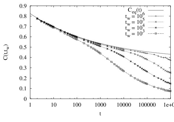
The relaxation function $S(t,t_{w})$ is just given by

S(t,t_{w})\equiv R(t,t_{w})=\beta^{-1}\lim_{\delta h\to 0}{\delta\langle m(t+t_{w})\rangle\over\delta h}\ ,

(17)

where $\delta m$ is the variation of the magnetization when we add a magnetic field $\delta h$ starting from time $t_{w}$ and $S(t,t_{w)}$ and $\chi(t_{w},\omega)$ are related by Fourier transform.

Naive scaling implies

C(t,t_{w)}=\hat{C}(t/t_{w}),\ \ \ \ \ \ R(t,t_{w)}=\hat{R}(t/t_{w})\,

(18)

The dependence on $t$ and $t_{w}$ of the previously defined functions is rather complex and cannot be computed from general principles.

It is convenient to examine directly the relation between $S$ and $C$ , by eliminating the time. At this end we plot parametrically $S(t,t_{w})$ versus $C(t,t_{w})\equiv q(t,t_{w})$ at fixed $t_{w}$ . The theory predicts that such a plot goes to a finite limit when $t_{w}\to\infty$ and we can extract from it information on the phase structure of equilibrium configurations. Using general arguments [6, 7, 8] one finds that when $t_{w}\to\infty$ ,

{dS\over dC}=X(C)=\int_{0}^{C}dqP(q)\ .

(19)

This equation is very important because it connects quantities that can be measured in the dynamics (l.h.s) to quantities that a defined at equilibrium (r.h.s.).

3.4 Three possible forms of fluctuation dissipation relations

The behavior of the system at equilibrium and the modification of the fluctuation dissipation theorem off-equilibrium are strongly related. These relations are summarized in fig. (5). In all the right panels the time decrease from right to left. At short times, the relaxation is a straight line (with slope -1), according to the fluctuation dissipation theorem. The interesting part is the one at left, where at large times, in the aging regime, the curve deviates from the previous straight line. The value of the relaxation at the point where the equilibrium regime ends is the linear response susceptibility $\chi_{LR}$ , while the value of the relaxation on the left-most point is the equilibrium susceptibility $\chi_{eq}$ .

•

A: There is an excess of noise with respect to equilibrium. The presence of noise without a corresponding response implies that the effective temperature $\beta X(C)$ is infinite.
•

B: A new and non trivial phenomenon, that should be present in structural fragile glasses and in some kind of spin glasses. The system has two temperatures, and both are finite. [32, 33, 34]. Often the higher temperature is near to the critical temperature.
•

C: A more complex phenomenon that is present in the mean field theory of some spin glasses. (e.g. in the original SK model). It correspond to the presence of a continuous range of temperatures in the aging region.

The presence of anomalies in the off-equilibrium regime in the plot of the response versus correlations (i.e. cases B and C) marks in a clear way the difference from the old picture (hysteresis). The experimental fact that in real spin glasses $\chi_{LR}\neq\chi_{eq}$ excludes case A.

In the case of Ising spin glasses with two body interaction in the mean field approximation we stay in case C. What happens in three dimensions is not clear. Numerical simulations [25, 26, 30, 4] on Ising model indicates that we stay in case C, while the experiments [35] see a clear effect of deviations from the case A that may indicate more case B.

From the theoretical viewpoint there are no firm commitments: although in infinite dimensions with a two-spin interaction we are in case C, the corrections due to the interaction among the fluctuations could bring the system in three dimensions in case B.

3.5 The physical meaning of the fluctuation dissipation relations

I will sketch a proof of the standard equilibrium fluctuation dissipation theorem using very simple and very general arguments.

The basic tools are equipartition law for harmonic oscillators and the zeroth law of thermodynamics; it states that:

•

Two bodies at thermal contact will eventually have the same temperature.
•

If $A$ has the same temperature of $B$ and $B$ has the same temperature of $C$ , $A$ has the same temperature of $C$ .
•

The heat goes from the body at higher temperature to the one at low temperature.

The equipartition law for harmonic oscillators states that the internal energy of an one dimensional harmonic oscillator is $kT$ .

Let us consider an harmonic thermometer. We have a spring coupled to a a quantity $M(t)$ of the system whose temperature we want to measure. The Hamiltonian of the thermometer is

H=\frac{1}{2}(p^{2}+\omega^{2}x^{2})+\epsilon\;xM(t)\ ,

(20)

and $\epsilon$ is very small (and the thermalization time diverges as $\epsilon^{-2}$ ). We want to compute the asymptotic value of the energy of the thermometer.

In order to be more precise, we can repeat the experiment many times and do the average over the different experiments. At $\epsilon=0$ we can define the correlation functions $C$ :

\langle M(t)M(t^{\prime})\rangle=C(t,t^{\prime})=C(t-t^{\prime})\ .

(21)

The last equality is true if the system is in a stationary state.

At the first order in $\epsilon$ we have

\langle M(t)\rangle=\epsilon\int_{0}^{t}dt^{\prime}x(t^{\prime})r(t^{\prime},t)\ ,

(22)

where $r$ is the response function and $r(t,t^{\prime})=r(t-t^{\prime})$ in a stationary state.

A long, but conceptually simple, computation tell us that the energy of the thermometer is $\omega$ independent and it is the correct one, if and only if we have the fluctuation dissipation relation:

r(t)=-\beta{dC(t)\over dt}\ .

(23)

If we introduce the relaxation function

R(t)=\int_{0}^{t}r(t^{\prime})dt^{\prime}\ ,

(24)

the fluctuation dissipation theorem becomes

{dR(t)\over dt}=-\beta{dC(t)\over dt}\ .

(25)

It may be convenient to eliminate the time and consider $R$ as a function of $C$ , e.g. to plot parametrically $R(t)$ as function of $C(t)$ . In this way the classical fluctuation dissipation theorem has a very compact form:

{dR\over dC}=-\beta\ .

(26)

Around 1993 [6, 7] it was showed that in some slightly off-equilibrium situations (e.g. during the ageing of the system) there is a generalized fluctuation dissipation relation.

{dR(t^{\prime},t)\over dt}=-\beta X(C(t^{\prime},t)){dC(t^{\prime},t)\over dt}\ ,

(27)

If at fixed $t^{\prime}$ we eliminate $t$ , we get:

{dR(t^{\prime},t)\over dC(t^{\prime},t)}=\beta X(C(t^{\prime},t))\ \ \ \ \ {dR\over dC}=\beta X(C).

(28)

The plot of $R(t^{\prime},t)$ versus $dC(t^{\prime},t)$ at fixed $t^{\prime}$ is not a straight line and becomes independent of $t^{\prime}$ for large $t^{\prime}$ . The function $\beta X(C)$ has the meaning of an effective temperature at non-equilibrium.

The function $X(C)$ can be computed at equilibrium in a subtle way: it is related both to existence on an exponential large number of equilibrium states and to the overlap distribution at equilibrium. If simple aging is valid we have that

	$\displaystyle R(t_{w},t)=f(t-t_{w})\ \mbox{for}\ t-t_{w}>>t_{w},$		(29)
	$\displaystyle R(t_{w},t)=g(t/t_{w}))\ \mbox{for}\ t-t_{w}=O(t_{w})\ .$

In other words, we cool the system at time zero and we make the observations around a time $t_{w}$ after cooling:

•

If the scale of time of the observations is small the results do not depend from the waiting time $t_{w}$ , and we see the usual microscopical temperature.
•

If the scale of time of the observations is comparable to $t_{w}$ , the results depend on the waiting time and we see an effective temperature that is higher that the microscopic one.

The physical interpretation is simple: the system being at non equilibrium must rearrange itself, and this produces an extra noise that does not have the adequate correspondence in the response of the system.

If we are at equilibrium

\langle M(t_{w})M(t)\rangle\equiv C(t_{w},t)=C(t-t_{w})

(30)

and only one long experiment is enough. If not (we are at off-equilibrium), you have to measure $M$ 100 times over 100 thermal histories to get an error on $C$ of 10%. In simulations and eventually in optics, you can do measures in parallel: e.g.

{\sum_{i=1,N}\sigma_{i}(t_{w})\sigma_{i}(t)\over N}=C(t_{w},t)\ .

(31)

3.6 Experimental results

Using the apparatus described in fig. (7), both the fluctuation and the dissipation has been measured on the same sample [35]. This has been done by cooling a spin glass sample from above to below the critical temperature. As far as the data show a sizable dependence on the waiting time the authors of ref. [35] have analyzed both the raw data have been and the called ageing part, where an extrapolation to infinite waiting time has been done,

The region where equilibrium FDT does not hold is not horizontal in fig. (8). The is not so much curvature in the non-FDT region: theoretical problem: only one temperature, not a continuos one. This is not in agreement with Ising simulation [30], may be it is in agreement with Heisenberg simulations.

The new off equilibrium fluctuation dissipation relations are extremely important for many reasons:

•

They are a first step toward the construction of a thermodynamics for slightly off equilibrium systems.
•

They provide a way to investigated in details the structure of the different equilibrium states.
•

Different theoretical models predict different forms of the function $X(C)$ and in this way FD experiments may better discriminate between different theories.

It would be extremely interesting to have precise measurements of these off equilibrium fluctuation dissipation relations in a variety of different materials as function of the external parameters. At the present moment most of the results come from theoretical models or from numerical simulations (in spin glasses, fragile glasses, colloids and granular materials).

The effect has been clearly observed in the brilliant experiment in spin glasses for one material. More systematic studied are missing. Some effects have been observed in colloids, glasses and granular materials, but not so clearly as in spin glasses. New experimental results are very welcome: they are not easy (the measurement of thermal noise in a non-stationary system is a rather difficult enterprise), but the results would be very interesting.

This difference between the simulations and the experiment may have two different origins:

•

The experiment and the numerical simulations do correspond to two different regimes: the time scales are quite different. Moreover, if experimentally we cool an high temperature system, thermalized domains grow with time and the maximum experimental reachable side is about 100. In simulations a compact system can be thermalized up to size 20.
•

The numerical simulations are mostly done on Ising systems while the experiment have been mostly done on a more Heisenberg systems with anisotropy an a long range tail of interactions (other systems are more complex); there are indications from other properties that the two systems behave in a different manner.

More extended numerical simulations and experimental results on other systems are needed to decide which picture is correct. One should also consider the possibility that the correlation length in the equilibrium limit remains fine, but very large (e.g. 1000 lattice units). In such a case one should see the effects of broken replica symmetries for times of human scale and only for astronomical times the anomaly should disappear. The possibility of this phenomenon is difficult to dismiss, but it would not jeopardize the interpretation of the experimental data using spontaneously broken replica theory.

In structural fragile glasses numerical simulations and strong theoretical arguments point to the fact that they should belong to case B. Unfortunately, although deviations from the equilibrium dissipation fluctuations dissipation relations have been observed in structural glasses, the situation is not so clear as for spin glasses.

4 Memory

Other impressive phenomena that happen mainly in spin glass are memory and rejuvenation (or oblivion). In the nutshell the magnetic response of the system depends on the history of the system in a very peculiar way. Some of the relevant experiments are shown in fig. (9,10). It is quite remarkable that we stop at the two temperatures only when cooling, not when heating, however one sees in fig. (10) the dips in $\chi^{\prime\prime}$ during both cooling and in heating.

We cannot discuss in detail these very interesting phenomena. We only remark that these effects are more difficult to understand for the following reasons:

•

Analytic computations are very difficult also in mean field theory.
•

The effects are much more pronounced for Heisenberg than Ising spins.
•

The effects are nearly invisible in simulations (mostly done for Ising spins).

A possible explanation could based on two hypothesis:

•

The free energy landscape at one temperature is not correlated to the free energy landscape at an other temperature, (temperature chaos).
•

The degrees of freedom that are active at one temperature, are frozen at lower temperature

5 The lowest critical dimension

The calculation of free energy increase due to an interfaces is a well known method to compute the lowest critical dimension for spontaneous symmetry breaking [38].

In the simplest case we can consider a system with two possible coexisting phases ( $A$ and $B$ ), with different values of the order parameter. For standard ferromagnets $A$ corresponds to spins up and $B$ corresponds to spins down.

We will study what happens in a finite system in dimensions $D$ of size $M^{d}\times L$ with $d=D-1$ . We put the system in phase $A$ at $z=0$ and in phase $B$ at $z=L$ . The free energy of the interface is the increase in free energy due to this choice of boundary conditions with respect to choosing the same phase at $z=0$ and $z=L$ In many cases we have that the free energy increase $\delta F(M,L)$ behaves for large $M$ and $L$ as:

\delta F(L,M)=M^{d}/L^{\omega}\ ,

(32)

where $\omega$ is independent from the dimension.

There is a critical dimension where the free energy of the interface is finite when both $M$ and $L$ go to infinity at fixed ratio:

D_{c}=\omega+1.

(33)

Heuristic arguments, which sometimes can be made rigorous, tell us that when $D=\omega+1$ , (the lowest critical dimension) the two phases mix in such a way that symmetry is restored. In most cases the value of $\omega$ from mean field theory is the exact one and therefore we can calculate in this way the value of the lower critical dimension. The simplest examples are the ferromagnetic Ising model $\omega=0$ and the ferromagnetic Heisenberg model $\omega=1$ .

For spin glasses the order parameter is the overlap $q$ . We consider two replicas of the same system described by a Hamiltonian:

H=H[\sigma]+H[\tau]\ ,

(34)

where $H$ is the Hamiltonian of a a single spin glass. We want to compute the free energy increase corresponding to imposing an expectation value of $q$ equal to $q_{1}$ at $z=0$ and $q_{2}$ at $z=L$ .

A complex computation gives (for small $|q_{1}-q_{2}|$ )

\delta F\propto ML(|q_{1}-q_{2}|/L)^{5/2}\propto L^{(D-5/2)}\ .

(35)

As a consequence, the naive prediction of mean field theory for the lower critical dimension for spontaneous replica symmetry breaking is $D_{c}=2.5$ .

These are testable prediction in Montecarlo on a $L^{D}$ system. If the same result is valid also at zero temperature, it may be checked by computing the ground state: One should find

\delta E\propto L^{(D-5/2)}\ .

(36)

I stress that these predictions are naive; corrections to the mean field theory are neglected, however n known cases these kind of computations give the correct result.

6 Conclusions

A strong effort should be done in order to have better quantitative predictions and a more precise comparison between theory and experiments. There are open problems in spin glasses, glasses and related fields where I would like to see a progress:

•

A systematic and careful experimental study of the fluctuation-dissipation relations is needed.
•

It would be important to obtain more precise understanding of the glass transition in structural fragile glass, and to get quantitative predictions on the behavior of the dynamics in the region where it is dominated by escapes from barriers.
•

New results should be obtained of the form of time behavior in non-equilibrium state, where only partial results are known.
•

In order to arrive to a precise assessment of the behavior of three dimensional spin glasses it would be very important to develop further the renormalization group approach and/or other theoretical or experimental techniques.

References

[1] P.W. Anderson, Ill condensed matter, edited by R. Balian, R. Maynard and G. Toulouse, (North-Holland 1983).
[2] Mézard, M., Parisi, G. and Virasoro, M.A. Spin Glass Theory and Beyond, World Scientific, Singapore, 1987
[3] G.Parisi, Field Theory, Disorder and Simulations, World Scientific, (Singapore 1992), Les Houches.
[4] E. Marinari, G. Parisi, F. Ricci-Tersenghi, J. Ruiz-Lorenzo and F. Zuliani, J.Stat. Phys. 98, 973 (2000).
[5] J.-P. Bouchaud, J. Phys. France 2 1705, (1992).
[6] L.F. Cugliandolo and J. Kurchan, Phys. Rev. Lett. 71, 173 (1993), J. Phys. A: Math. 27, 5749 (1994).
[7] S. Franz and M. Mézard Europhys. Lett. 26, 209 (1994).
[8] S. Franz, M. Mézard, G. Parisi, L. Peliti, Phys. Rev. Lett. 81, 1758 (1998), J. Stat. Phys. 97 459 (1999) .
[9] D.Sherrington and S.Kirkpatrick, Phys. Rev. Lett., 35, 1792, (1975).
[10] L. Viana and A. J. Bray, J. Phys. C 18 3037 (1985).
[11] Mézard and G. Parisi, Eur.Phys. J. B 20 (2001) 217, J. Stat. Phys 111 (2003) 1.
[12] S. Franz and M. Leone, J. Stat. Phys 111 (2003) 535
[13] Edwards and Anderson, J. Phys F5 (1975) 965.
[14] D.J. Thouless, P.A. Anderson and R. G. Palmer, Phil. Mag. 35, 593 (1977).
[15] A.J. Bray and M.A. Moore, J. Phys. C 13, L469 (1980).
[16] A. Cavagna, I. Giardina, G. Parisi and M. Mezard, J. Phys. A 36 1175 (2003).
[17] T. Aspelmeier, A. J. Bray, M. A. Moore, Phys. Rev. Lett. 92, 087203 (2004)
[18] Crisanti, L. Leuzzi, G. Parisi, and T. Rizzo, Phys. Rev. B 68, 174401 (2003).
[19] A. Cavagna, I.Giardina, G. Parisi, J. Phys. A 30 (1997) 7021, Phys. Rev. Lett. 92, 120603 (2004), Phys. Rev. B 71 024422 (2005).
[20] A. Annibale, A. Cavagna, I.Giardina, G. Parisi, Phys. Rev. E 68, 061103 (2003).
[21] A. Crisanti and T. Rizzo, Phys. Rev. E 65 (2002) 046137.
[22] T. Rizzo, J. Phys. A 38 3287 (2005).
[23] G. Parisi, Proceedings of the Les Houches summer school 2005 .
[24] R. Monasson, Phys. Rev. Lett. 75 (1995) 2847.
[25] E. Marinari, G. Parisi and J.J. Ruiz-Lorenzo, in Spin Glasses and Random Fields, ed. by P. Young (World Scientific, Singapore 1998).
[26] E. Marinari, F. Zuliani J. Phys. A 32, 7447 (1999).
[27] C. Djurberg, K. Jonason and P. Nordblad, Eur. Phys. J. B 10, 15 (1998).
[28] E. Marinari, G. Parisi, J. Ruiz-Lorenzo, and F. Ritort, Phys. Rev. Lett. 76, 843 (1996).
[29] Y.G. Joh, R. Orbach, G.G. Wood, J. Hammann, E. Vincent, Phys. Rev. Lett. 82, 438 (1999), J. Phys. Soc. Jpn. 69, Suppl. A, 215 (2000).
[30] E. Marinari, G. Parisi, F. Ricci-Tersenghi, and J.J. Ruiz-Lorenzo J. Phys. A 31, 2611 (1998).
[31] G. Parisi, F. Ricci-Tersenghi, and J.J. Ruiz-Lorenzo, Eur. Phys. J. B 11, 317 (1999).
[32] L. Cugliandolo, J. Kurchan, L. Peliti, Phys. Rev. E 55, 3898 (1997).
[33] S. Franz and M.A. Virasoro, J. Phys. A: Math. and Gen. 33, 891 (2000).
[34] G. Parisi, J. Phys. A 36 10773 (2003), Europhys. Lett. 65, 103 (2004)
[35] D. Hérisson and M. Ocio, Phys. Rev. Lett. 88, 257202 (2002).
[36] K. Jonason, E. Vincent, J. Hammann, J. P. Bouchaud, and P. Nordblad, Phys. Rev. Lett. 81, 3243 (1998).
[37] J.-P. Bouchaud, L. Cugliandolo, J. Kurchan., M Mézard, Physica A 226, 243 (1996), in Spin glasses and random fields, A.P.Young editor, Worlds Scientific 1998.
[38] S. Franz, G. Parisi, M.A. Virasoro , J. Phys. Frannce , I 4, 1657 (1994).