Grassmannian spectral shooting
Abstract.
We present a new numerical method for computing the pure-point spectrum associated with the linear stability of coherent structures. In the context of the Evans function shooting and matching approach, all the relevant information is carried by the flow projected onto the underlying Grassmann manifold. We show how to numerically construct this projected flow in a stable and robust manner. In particular, the method avoids representation singularities by, in practice, choosing the best coordinate patch representation for the flow as it evolves. The method is analytic in the spectral parameter and of complexity bounded by the order of the spectral problem cubed. For large systems it represents a competitive method to those recently developed that are based on continuous orthogonalization. We demonstrate this by comparing the two methods in three applications: Boussinesq solitary waves, autocatalytic travelling waves and Ekman boundary layer.
Key words and phrases:
Grassmann manifolds, spectral theory, numerical shooting2000 Mathematics Subject Classification
65L15, 65L101. Introduction
We introduce a new numerical method for solving high order linear spectral problems by shooting and matching. The numerical construction of pure-point spectra is important in determining the linear stability of coherent structures. Examples of such structures are: ground and higher excited states of molecules in quantum chemistry (Johnson [56], Hutson [51], Gray and Manopoulous [39], Manopoulous and Gray [69], Chou and Wyatt [23, 24], Ledoux [64], Ledoux, Van Daele and Vanden Berghe [65], Ixaru [55]); nonlinear travelling fronts in reaction-diffusion such as autocatalysis or combustion (Billingham and Needham [9], Metcalf, Merkin and Scott [72], Doelman, Gardner and Kaper [31], Terman [96], Gubernov, Mercer, Sidhu and Weber [41]); nerve impulses (Alexander, Gardner and Jones [2]), neural waves (Coombes and Owen [25]); solitary waves or steady flows over compliant surfaces (Pego and Weinstein [82], Alexander and Sachs [3], Chang, Demekhin and Kopelevich [21], Kapitula and Sandstede [57], Bridges, Derks and Gottwald [14], Allen [4], Allen and Bridges [5]); laser pulses (Swinton and Elgin [95]); nonlinear waves along elastic rods (Lafortune and Lega [62]); ionization fronts (Derks, Ebert and Meulenbroek [28]) or spiral waves (Sandstede and Scheel [89]).
For such problems the matching condition is typically a discriminant known as the Evans function (Evans [34], Alexander, Gardner and Jones [2]) or miss-distance function (Pryce [85], Greenberg and Marletta [39]). It measures the degree of (possibly transversal) intersection of the stable and unstable solution subspaces satisfying the longitudinally separated far field boundary data. The stable subspace decays in the direction of wave propagation whilst the unstable subspace decays in the opposite direction. Equivalently, the Evans function is the determinant of the set of solution vectors spanning both subspaces. With this end-goal matching condition in mind, the problem boils down to how to numerically construct the solution subspaces in a robust fashion, as well as where to match longitudinally. This is especially difficult for large scale problems. These might either emerge from high order systems, or more specifically, we envisage the stability of nonlinear travelling waves with multi-dimensional structure; for example wrinkled fronts travelling in a fixed longitudinal direction. The transverse structural information can be projected onto finite dimensional transverse basis, generating a large linear spectral problem posed on the one-dimensional longitudinal coefficient function set (see Ledoux, Malham, Niesen and Thümmler [66]). Hitherto such large problems could not be solved by shooting and matching and were resolved by projecting the whole problem onto a finite basis and solving the resulting large algebraic eigenvalue problem. However recently, in the context of the Evans function, Humpherys and Zumbrun [49] proposed continuous orthogonalization as a viable approach to help make large scale problems amenable to shooting and matching. Here we provide our own answer.
We propose the new Grassmann Gaussian elimination method (GGEM) which resolves several numerical problems all in one, in particular it:
- (1)
Evolves the solution along the underlying Grassmann manifold avoiding representation singularities.
- (2)
Retains analyticity in the spectral parameter.
- (3)
Allows for matching anywhere in the longitudinal computational domain.
- (4)
Has polynomial complexity, operations are of the order of the size of the system cubed.
- (5)
Naturally evolves the solution in what in practice is the optimal coordinate representation (generated by optimal partial pivoting).
For each property what is new, expected, proved, numerically observed, and its context?
First, evolving the solution subspaces, considered as curves in the Grassmann manifold is not new for autonomous problems—see Hermann and Martin [44, 45, 46, 47, 48], Martin and Hermann [71] Brockett and Byrnes [18], Shayman [92], Rosenthal [87], Ravi, Rosenthal and Wang [86], Zelikin [100], Abou–Kandil, Freiling, Ionescu and Jank [1] and Bittanti, Laub and Willems [12]. Using Riccati systems to solve nonautonomous spectral problems is also not new—see Johnson [56], Hutson [51], Pryce [85], Manopoulous and Gray [69], Gray and Manopoulous [38] and Chou and Wyatt [23, 24]. Here Riccati systems correspond to the flow of the linear spectral problem projected onto the Grassmann manifold with a fixed coordinate patch representation—see Schneider [91]. Also see Schiff and Shnider [90] and Chou and Wyatt [24] who use this connection to integrate Riccati systems through singularities.
That we have a numerical method that avoids representation singularities for nonautonomous systems is new. The idea is as follows. Given data that lies in a suitable coordinate patch of the Grassmann manifold, pullback to the Stiefel manifold. Evolve the solution one steplength along the Stiefel manifold either directly using a Runge–Kutta method or a Lie group method. Then project onto a suitable and possibly different coordinate patch of the Grassmann manifold using optimal Gaussian elimination. In this last step, the practical method we propose picks a quasi-optimal coordinate patch in which to best represent the solution in the Grassmann manifold (see below and Section 5).
Note that on first inspection the Stiefel manifold is the direct natural setting for the stable and unstable solution subspaces. Afterall in each case we have to construct the full set of solutions to a large system of differential equations satisfying the correct respective asymptotic boundary conditions in the far field. Each solution set represents a curve in the Stiefel manifold of dimension commensurate with the size of the solution set. That the spectral problems are linear means that all the relevant spectral information can be reconstructed from the flow in the corresponding Grassmann manifold. That the matching condition is determinental, means that we only need the Grassmann flow information—see Martin and Hermann [71] and Brockett and Byrnes [18] where this reduction was first considered for autonomous linear control problems (in practice we will also need to retain a complex scalar field to ensure analytic dependence on parameters). This reduction is crucial because long-range integration along the Stiefel manifold has been problematic (due to multiple distinct exponential growth and decay rates) and one of the simplest resolutions in the Evans function context was to use Plücker coordinates—whilst ignoring the Plücker relations (more on these below).
Second, retaining analyticity away from the essential spectrum is standard for any shooting method; we prove analyticity in Section 6. This allows for a global search for eigenvalues in that region by numerically computing the change in argument of the Evans function round any closed contour. Invoking the argument principle, this integer value represents the number of zeros of the Evans function, and hence the number of eigenvalues counting multiplicity, inside the contour; see Brockett and Byrnes [18], Alexander, Gardner and Jones [2] and Ying and Katz [99].
Third, that our method allows matching anywhere in the longitudinal domain is new. We provide substantive numerical evidence. Previously, other than in trivial cases, most numerical practioners used the common-sense rule of thumb of integrating the spectral problem from both ends of the longitudinal domain and matching at a point roughly centered on the front (which is assumed to be localized). When solving the linear problem with Plücker coordinates, it was first important to rescale for the far field spatial behaviour to neutralize its total exponential growth. Integrating from the far field initial conditions (a subset of the spatial eigenvectors), the solution remains roughly constant until the coefficient matrix starts to reveal its nonautonmous character due to the integration step impinging on the front. Accuracy is retained whilst integrating through the front, but thereafter the problem becomes stiff. The issue is that the numerical methods cannot resolve the simultaneous exponential growth and decay character associated with the other far-end stable and unstable subspaces.
Fourth, having polynomial complexity is essential and we provide here a new alternate. After Humpherys and Zumbrun [49] introduced their continuous orthogonalization method in this context, which also has polynomial complexity, any new numerical spectral shooting method should have this property and also be competitive. Previous successful methods used Plücker coordinates, ignoring the quadratic Plücker relations (see Section 2). They solved the flow for the corresponding linear vector field in the higher dimensional Plücker embedding space. Details of this Plücker coordinate or compound matrix approach can be found in, for example, Alexander and Sachs [3], Brin [16, 17] and Allen and Bridges [5]. Unfortunately the number of Plücker coordinates typically grows exponentially with the order of the original system, and so this approach cannot be used for medium to large order systems. However the continuous orthogonalization method of Humpherys and Zumbrun, and our method, are especially suited to large scale problems.
Fifth, our method for dynamic practical optimal coordinate representation is new. Given data on the Stiefel manifold, for example generated by advancing the solution one steplength along the Stiefel manifold, how can we project down onto the Grassmann manifold using the best representation patch possible? The idea is as follows. The natural map projection from the Stiefel to the Grassmann manifolds is a linear fractional map (Milnor and Stasheff [74]; Martin and Hermann [71]). This map represents the action of equivalencing by transformations whose rank matches that of the Stiefel manifold (this takes us from the space of frames to the space of spaces spanning those frames). The Stiefel manifold has a non-square matrix representation. Projection onto the Grassmann manifold corresponds to equivalencing by a full rank submatrix of the non-square Stiefel matrix—this renders the corresponding submatrix as the identity matrix. We are free to choose which submatrix to equivalence by, each distinct choice corresponds to the matrix representation of a coordinate patch on the Grassmann manifold. We can use Gaussian elimination, via elementary column operations, to render any given full rank submatrix of the Stiefel matrix as the identity matrix. The key is to try to pick the full rank submatrix which has the largest determinant—this corresponds to choosing the Grassmannian patch that gives the best representation for the projection from the Stiefel to Grassmann manifold. Ideally we would check the size of every full rank submatrix of the Stiefel matrix and equivalence by the one with the largest determinant. However this is an NP problem (equivalent to using the Plücker coordinates described above). We provide a practical solution of polynomial complexity. The method maximises the pivot used at each step of the Gaussian elimination process. In the current context, we call it quasi-optimal Gaussian elimination.
Our paper is organised as follows. In Section 2, we provide a tailored review of Grassmann manifolds and their representation. We then show, in Section 3 how flows generated by linear vector fields on the Stiefel manifold, produce a natural flow on the underlying Grassmann manifold that is decoupled from the flow through the remaining fibres. We subsequently show how this leads to using Riccati systems to resolve spectra, but that singularities that develop in the Riccati flows present spectral matching problems. In Section 4 we introduce two new practical approaches to avoiding these representation singularities. One is the idea behind our main method, the Grassmann Gaussian elimination method. The other is a modification of the Riccati approach that changes the coordinate patch when deemed necessary. Also in this section we show the connection between the Riccati and continuous orthogonalization approaches. We present our proposed Grassmann Gaussian elimination method fully in Section 5, including details of how in practice to choose the quasi-optimal Grassmannian coordinate representation patch. We review the Evans function in Section 6 and discuss further simple practical numerical refinements that retain analyticity and prevent potential numerical overflow. We then implement and compare all the competing numerical methods in Section 7 in three distinct applications. Finally in Section 8 we conclude and present future directions.
2. Review: Grassmann manifolds
2.1. Grassmann and Stiefel manifolds
A -frame is a -tuple of linearly independent vectors in . The Stiefel manifold of -frames is the open subset of of all -frames centred at the origin. The set of dimensional subspaces of form a complex manifold called the Grassmann manifold of -planes in (see Steenrod [88, p. 35] or Griffiths and Harris [40, p. 193]).
The fibre bundle is a principle fibre bundle. For each in the base space , the inverse image is homeomorphic to the fibre space which is a Lie group—see Montgomery [76, p. 151]. The projection map is the natural quotient map sending each -frame centered at the origin to the -plane it spans—see Milnor and Stasheff [74, p. 56].
2.2. Representation
Following the exposition in Griffiths and Harris [40], any -plane in can be represented by an matrix of rank , say . Any two such matrices and represent the same -plane element of if and only if for some (the -dimensional subspace elements are invariant to rank closed transformations mapping -planes to -planes).
Let denote a multi-index of cardinality . Let denote the -plane in spanned by the vectors and
In other words, is the set of -planes such that the submatrix of one, and hence any, matrix representation of is nonsingular (representing a coordinate patch labelled by ).
Any element of has a unique matrix representation whose th submatrix is the identity matrix. For example, if then any element of can be uniquely represented by a matrix of the form
where for and . Conversely, a matrix of this form represents a -plane in . Each coordinate patch is an open, dense subset of and the union of all such patches covers . For each , there is a bijective map given by
Each is thus a local coordinate chart for the coordinate patch of . For all , if and is the th submatrix of , then . Since represents the transformation between representative patchs and depends holomorphically on , we deduce is holomorphic. Note that has a structure of a complex manifold (see Griffiths and Harris [40, p. 194]). Further the unitary group acts continuously and surjectively on . Hence is compact and connected. Lastly, the general linear group acts transitively on and it is a homogeneous manifold isomorphic to (see Chern [22, p. 65] or Warner [97, p. 130]).
2.3. Plücker embedding
There is a natural map, the Plücker map,
that sends each -plane with basis to ; here denotes the complex projective space of dimension . See Griffiths and Harris [40] or Coskun [26] for more details. If we change the basis, the basis for the image changes by the determinant of the transformation matrix. Hence the map is a point in . We can recover from its image as the set of all vectors such that . Further, a point of is in the image of if and only if its representation as a linear combination of the basis elements of , consisting of all possible distinct wedge products of a -dimensional basis in , is completely decomposable. Hence the image of is a subvariety of of completely decomposable elements. It can also be realized as follows. A natural coordinatization of is through the determinants of all the submatrices of , normalized by a chosen minor characterized by an index , hence . These minor determinants—the Plücker coordinates—are not all independent, indeed, they satisfy quadratic relations known as the Plücker relations (which may themselves not all be independent). The image of the Plücker map is thus the subspace of cut out by the quadratic Plücker relations.
3. Grassmannian flows
3.1. Tangent space decomposition
Recall that we can consider the Stiefel manifold as a principle fibre bundle . Our goal here is to characterize the induced decomposition of the tangent space for . We can decompose the tangent space into horizontal and vertical subspaces (see, for example, Montgomery [76, p. 149])
The horizontal subspace is associated with the tangent space of the Grassmannian base space, while the vertical subspace is associated with the fibres homeomorphic to . Let us choose the coordinate patch representation for for some . Let denote the projection matrix of size that contains zeros everywhere except at positions for where it contains ones. Note that one can additively decompose any given tangent vector . Hence we have
3.2. Fibre bundle flow
Suppose we are given a vector field on the Stiefel manifold
for any where . Fixing a coordinate patch for for some we can always decompose into
where . Let , , and denote the , , and submatrices of , respectively.
Theorem 1.
The flow governed by generates a coupled flow in the base space and fibres : if for a given fixed , the flows in the coordinate chart variables , and rank transformations , are
where we now think of , , and as functions of , and .
Proof.
Using that the ordinary differential system becomes
where represents the submatrix obtained by restricting the matrix to its th columns. Applying the projections and to both sides of this equation, respectively generates the equations for and shown. Note that is the projection of onto its th rows, as well as its image under the coordinate chart . ∎
3.3. Riccati flow
A natural decoupling of the flow on the base space from the flow on the fibres occurs when the vector field is linear, i.e. when
The following corollary is immediate from Theorem 1.
Corollary 1.
If the vector field is linear so that only, then:
- (1)
The flow on the base space decouples from the flow evolving through the fibres —the flow in the fibres is slaved to that in the base space;
- (2)
For a fixed coordinate patch index by , in the coordinate chart variables , the flow is governed by the Riccati differential system:
Suppose we are required to determine the flow generated by a linear nonautonomous vector field defined on the Stiefel manifold . The first conclusion in the corollary implies that all the relevant information is carried in the flow in the Grassmann manifold , and the flow through the fibres can be completely determined a-posteriori from the Grassmannian flow. The second conclusion suggests that if we fix a coordinate patch, then the flow in the Grassmannian can be determined from the solution to the Riccati system for . If required, we can solve the differential system for in Theorem 1 to determine , thereby completely resolving the flow generated by the linear vector field on the Stiefel manifold. Provided remains finite, this approach in fact works.
The problem is that, though must be globally finite as it is generated by a linear vector field (with globally smooth coefficients), the Riccati solution itself can become singular in a finite integration interval. Of course simultaneously the determinant of itself becomes zero. The solution on the Grassmannian does not become singular. The issue is representation. (Note that the flow on is linear but rank is not preserved because its coefficients depend on the Riccati flow.)
The Riccati flow is a flow in a given fixed coordinate chart indexed by , which is chosen at the start of integration. Given an initial element in , we pick a (good) coordinate patch for , this fixes the Grassmannian representation . Projecting onto the th rows of , or equivalently looking at the image under the coordinate chart , generates . The Riccati flow is the flow in the Euclidean chart image space . Each coordinate patch is dense in . Therefore in numerical computations, the Riccati solution is likely to leave and return to the patch across any discrete integration step that staddles a representation singularity (generating a large but finite solution the other side).
With this in mind, Schiff and Shnider [90] suggested the following method that integrates through singularities in the Riccati flow. Fix a coordinate patch with index . The general linear group acts transitively on (and also ): the left Lie group action is defined by . For we set
The Möbius Lie group action is defined by , where is the quotient map . Explicitly, if represents the submatrix of , we have:
Thus, given data in the Euclidean chart image space , pullback to the Lie group , to the identity element , using the Möbius Lie group action map . Advance the solution across one integration step in the Lie group generating the element . Schiff and Shnider used a Neumann/Runge–Kutta method to do this, but a Lie group method could also be used. Now push forward to using the Möbius Lie group action map. This takes you back to the chart corresponding to the original coordinate patch .
This method integrates through singularities in the Riccati flow. However, we are still left with another associated practical problem. If the linear vector field depends on a parameter we wish to vary, the singularities in the Riccati flow can drift in the domain of integration and impinge on the matching position.
4. Practical Grassmann integration
Our goal in this section is construct numerical methods that integrate the flow associated with the push forward of the linear vector field onto the Grassmannian manifold, whilst avoiding the representation singularities that occur in the Riccati approach. The solution is to change patch continuously in some optimal fashion or whenever the coordinate patch becomes a poor representation.
The following diagram helps map out the two new strategies we suggest.
4.1. Continuous optimal patch evolution
The idea behind the Grassmann Gaussian elimination method (GGEM) is this. Given data in that lies in a given patch identified by , pullback to the Stiefel manifold using the identity map—note —so . Advance the solution one integration step along the Stiefel manifold , using say a classical Runge–Kutta method, thus generating the element .
Now with the next step solution on the Stiefel manifold, we use quasi-optimal Gaussian elimination with partial pivoting (QOGE) to decompose and project onto the coordinate patch producing the element . The quasi-optimal Gaussian elimination process (described in Section 5) picks out a suitable coordinate patch to represent the solution, which may be different than the original patch .
To ensure we numerically remain with the Stiefel manifold, rather than use a Runge–Kutta method, we might use a Lie group method as follows (see Munthe–Kaas [77]). Pullback the data from the Stiefel manifold to the general linear group , via the action map . The corresponding element in is naturally the identity element . Subsequently pullback, via the exponential map, to the zero element in the corresponding Lie algebra, i.e. . Evolve the solution on the Lie algebra to using the Magnus expansion (Magnus [68]; also see Iserles, Munthe–Kaas, Nørsett and Zanna [54]). Pushforward from to , via the exponential map, producing the Lie group element . Now pushfoward to the Stiefel manifold via the Lie group action map . For more details on Lie group methods for Stiefel manifolds, see Krogstad [61] and Celledoni and Owren [20].
4.2. Riccati flow with patch swapping
Since we are interested in constructing the flow generated by the push forward of the vector field onto the Grassmann manifold, we can avoid singularities in any given Riccati system chart flow associated with a given Grassmannian coordinate patch, by simply changing patch when the solution representation appears to become poor. In particular, we could either change the coordinate patch when the:
- •
Norm becomes too large (the easier and preferred approach we take);
- •
Determinant becomes too small (this involves constructing as integration proceeds and we want to avoid carrying information unnecessarily).
Hence if say exceeds a prescribed tolerance at the end of one step, to change patch, we apply the quasi-optimal Gaussian elimination method (QOGE) to the matrix . This identifies a new patch and index to use for the next set of successive steps until becomes too large again, and so forth.
4.3. Drury–Oja flow
There is a close connection between the Riccati flow in Corollary 1 and the continuous orthogonalization method of Humpherys and Zumbrun [49], proved by direct comparison.
Lemma 1.
If satisfies the Riccati flow and satisfies , then for any index , we have that satisfies the Drury–Oja flow: .
Humpherys and Zumbrun [49] derive this flow by a -decomposition of the solution to the linear, spectral, globally bounded flow . We can think of this continuous orthogonalization method as generating an approximate flow on the Grassmann manifold whilst evolving the coordinatization (see Edelman, Arias and Smith [33]; Bindel, Demmel and Friedman [11]). It is also known as a Drury–Oja flow (see Drury [32], Oja [80], Yan, Helmke and Moore [98], Bridges and Reich [15], Dieci and Van Vleck [30] and Hairer, Lubich and Wanner [42, p. 136]). The determinant of the upper triangular matrix, , grows exponentially. Thus, since it is nonzero in the far field, we know it remains nonzero in the whole integration interval . Consequently, is globally finite on , i.e. there are no singularities in the Drury–Oja flow.
There is a natural Lie algebra action on the Stiefel manifold of orthonormal -frames, , generated by the map , for and . If , the flow on the Lie algebra that generates the Drury–Oja flow on is governed by . We could use this to construct a numerical method that preserves orthonormality of .
5. Grassmann Gaussian elimination method
5.1. Algorithm
The Grassmann Gaussian elimination method using a Lie group method on the Stiefel manifold (GGEM-LG), proceeds as follows:
- (1)
Suppose initially we are given data in the coordinate patch .
- (2)
Across the integration interval , compute using the Magnus expansion—we recommend the fourth order Magnus expansion.
- (3)
Compute .
- (4)
Apply quasi-optimal Gaussian elimination (QOGE) (outlined below) to ; this generates the solution in the coordinate chart , and the rank matrix we have effectively equivalenced by.
Across the integration interval , we could generate from by solving the flow on the Stiefel manifold using a classical Runge–Kutta step (GGEM-RK). Both algorithms are summarized in the following diagram.
How much of do we retain at each step? We address this in Section 6.4.
5.2. Quasi-optimal Gaussian elimination
To project the endpoint solution in the Stiefel manifold onto a quasi-optimal coordinate patch, say , we use a Gauss–Jordan approach. This entails using elementary column operations and optimal pivoting, until a specified submatrix of becomes the identity matrix (we naturally assume ). To be more explicit about what we mean by optimal pivoting, we outline the procedure:
- (1)
Look for the largest term in magnitude in . Nominate this term as the pivot term and suppose this occurs in row , column . Use elementary column operations with this term, , as the pivot to render all the other terms in that row equal to zero. Finally, use the elementary column operation of scalar multiplication to render the pivot term itself equal to one. Let us call the resulting matrix ; we can write (see for example Meyer [73])
where the elementary column operations performed are encoded in the elementary matrix . To be precise, we can write
where for the elementary matrix encodes the following elementary column operation on column :
For the elementary matrix encodes the elementary column operation . In summary, the matrix has value one at position and otherwise zeros in row ; and we have .
- (2)
In the submatrix of identified by excluding row and column , look for the largest term in magnitude. Again nominate this term as the pivot term and suppose this occurs in row (which will be distinct from ), and column (which is distinct from ). Here and refer to the row and column relative to the original matrix . Use elementary column operations with this term, , as the pivot to render the terms in row and columns of equal to zero. Again use the elementary column operation of scalar multiplication to render the pivot term itself equal to one. Let us call the resulting matrix ; we can write
where the elementary column operations performed on are encoded in the elementary matrix . Again, to be precise, we can write
where for the elementary matrix encodes the following elementary column operation on column :
Note that in our expression for above we could have either or . For then encodes the elementary column operation . In summary, the resulting matrix has value one at positions and and otherwise zeros in row , and zeros in row in columns ; and we have .
- (3)
Continue this process. Focus on the submatrix of identified by excluding the rows and columns ; look for the largest term in magnitude. Nominate this term as the pivot term—suppose it occurs in row and column , relative to the original matrix , and so forth. On completing the final th step in this process, we will have
where
The final matrix will have ones in positions , for . In row it will have zeros in columns . We set
- (4)
Perform column swaps in so that column becomes column , column becomes column , and so forth so that finally column is forced to be column . These column swaps can be encoded in the elementary matrix with . The resulting matrix is given by
The submatrix of given by
is lower triangular with ones on the diagonal. Finally we set
In practice of course, we do not compute , but continue performing elementary column operations on so that the submatrix becomes the identity matrix, thus generating . Hence we have effectively performed the decomposition
where , and in particular
Note that if then the entries in and , produced as a result of this process, will all be finite. Further if depends analytically on a parameter, then the product naturally does as well. Lastly we remark that we could have performed alternative elementary column operations of the form (we do not include the scalar multipication operations here) with the result that .
5.3. Complexity
The complexity of the quasi-optimal Gaussian elimination algorithm, dominated by the search for the largest elements in the successively decreasing submatrices of , is of order . The method is a practical approach to maximize the determinant of the submatrix removed from . It will not in general choose the submatrix with the largest determinant—hence the label quasi-optimal. This could be achieved by searching through all the submatrices of , i.e. all the Plücker coordinates, but this has complexity of order choose . An interesting question here is whether there is an efficient way to use the Plücker relations to reduce this complexity?
6. Spectral problems
6.1. Linear Stiefel flow
Consider the linear spectral problem on :
We assume there exists a subdomain containing the right-half complex plane, such that for there exists exponential dichotomies on and with the same Morse index in each case (see Henry [43] and Sandstede [88]). Let denote the matrix whose columns are solutions to the spectral problem and which span the unstable manifold section at . Let denote the matrix whose columns are the solutions which span the stable manifold section at .
6.2. Matching
The values of spectral parameter for which the columns of and columns of are linearly dependent on are pure-point eigenvalues. The Evans function is the measure of the degree linear dependence between the two basis sets and , i.e. of the degree of transversal intersection between the unstable and stable manifolds (see Alexander, Gardner and Jones [2]; Nii [79]):
It is analytic in . In practice we drop the non-zero, scalar exponential prefactor and evaluate the Evans function at a matching point .
There are other matching criteria measuring the degree of intersection between subspaces that do not use the determinant: for example computing the angle between subspaces as suggested by Björck and Golub [13] or computing the smallest eigenvalue as suggested by Hutson [51] and Ixaru [55]. Both these latter techniques might be important for large systems when computing the determinant could be an unstable process, indeed, we investigate them in this context in Ledoux, Malham, Niesen and Thümmler [66]. However in both cases the magnitude of a function of the spectral parameter is computed, whose zeros correspond to eigenvalues. Hence we must search for touchdowns to zero in the complex parameter spectral plane which can be problematic. For the examples we consider here, which are not too large, using the determinant suffices.
6.3. Initialization
We construct the matrix whose columns are the eigenvectors of corresponding to eigenvalues with a positive real part (see Humpherys and Zumbrun [49] and also Humpherys, Sandstede and Zumbrun [50] for how to preserve analyticity with respect to the spectral parameter ). In practice, integration starts at for some suitable, usually negative, value of . Analogously we construct the matrix whose columns are the eigenvectors of corresponding to eigenvalues with a negative real part. Again, in practice, we integrate backwards from for some suitable, usually large and positive, value of .
6.4. GGEM matching and analyticity
To compute we start with at and integrate centrally towards . Our goal in this section is to show that we only need the determinant of the rank transformations in the GGEM method described at the beginning of Section 5, to retain analyticity for the Evans function in . Since the procedure is the same in both intervals we will describe it for the generic interval for starting with value at . Suppose we use successive computation subintervals in where . We label the nodal solution values at as .
At the start , perform quasi-optimal Gaussian elimination (QOGE) on to obtain the decomposition
As we shall see, we do not need to actually store , but only .
Let denote an approximation to the flow-map across to the linear system . We assume that preserves analytic dependency on , so that the next step solution value analytically depends on if does. For example, in the case of GGEM-LG then and most straightforward Magnus based integrators will naturally preserve analyticity with respect to . Similarly most simple Runge–Kutta methods used to generate , or directly generate the next step solution value , will preserve analyticity.
Our numerical procedure would proceed as follows. Across we have
where in the last step we applied QOGE to the matrix . Subsequently, across we have
where we applied QOGE to . Repeating this argument across the subsequent intervals for , we get the following approximation to :
where . Naturally the product depends analytically on .
Returning to the separate interval calculations on , we see that by the procedure just outlined we can generate the solution approximations
The number of integration steps can of course be different in each interval. Hence, after dropping the exponential prefactor and fixing the matching point to be , the Evans function can be approximated by where
This is an analytic function of . Indeed as we hinted previously, at each computation step we need only store and the value
which gets updated at each step by simply multiplying the previous step value by the complex scalar determinental factor for current step. Hence to preserve analyticity for the Evans function using GGEM we must generate an approximate flow on .
6.5. Scaled GGEM
The scalar determinental factor just described, that we update at each step, grows exponentially. This would be tempered by the scalar exponential prefactor in the definition of the Evans function. An accurate practical procedure here is as follows (to be applied with due care). When integrating in the interval , at each step, divide the scalar determinental factor in GGEM by , where is the stepsize, and the are the (spatial) eigenvalues, with positive real part, of . When integrating in the interval , at each step, divide the scalar factor by , where the are the eigenvalues, with negative real part, of .
To see that this normalization is appropriate, we recall the Plücker coordinates of Section 2. After applying the optimal Gaussian elimination algorithm to the th row elements of are themselves Plücker coordinates; normalized by . The th row elements of and , can be used to reconstruct the remaining Plücker coordinates through the homogeneous, quadratic Plücker relations. Hence the Plücker coordinates, or complete set of minors, of and differ by a factor . It is well known that if the original vector field on is linear, then the Plücker coordinates corresponding to satisfy a (larger) linear system of equations. In the left far field the coordinates thus grow exponentially, in fact with growth rate ; hence our recommendation to divide by the exponential factor suggested (with an analogous argument for the right far field). See Alexander, Gardner and Jones [2], Alexander and Sachs [3], Brin [16, 17] or Allen and Bridges [5] for more details.
7. Applications
We present some numerical results for three different applications. The three applications reduce to the solution of a system showing multiple distinct exponential growth and decay rates in the stable and unstable subspaces, respectively. We show that our approach resolves this numerical obstacle successfully and can compete with the continuous orthogonalization method of Humpherys and Zumbrun [49].
7.1. Algorithms
We implement six different algorithms as follows.
(1) Riccati-RK: Riccati method with fixed coordinatization with the flow of the Riccati vector field approximated by the classical fourth order Runge–Kutta method. We generically chose the coordinatization labelled by and for the left-hand and right-hand intervals, respectively. Hence if and denote the unstable and stable subspaces of and , respectively, then we set
where denotes the submatrix of . We integrate the Riccati equation outlined in Corollary 1 in the two intervals and evaluate the modified Evans function
Provided neither Riccati flow becomes singular, this Evans function is analytic in the spectral parameter .
(2) Möbius–Magnus: Uses the Schiff and Shnider approach to integrate through singularities, combined with a Lie group method to advance the solution on the general linear group, as described at the end of Section 3. The same generic fixed coordinate charts are used as for the Riccati-RK method above. Over the integration interval with an equidistant mesh stepsize , we advance the solution on the Lie algebra using the fourth order Magnus method
with the two Gauss–Legendre points (see Iserles, Marthinsen and Nørsett [52])
We then compute the Möbius map to advance the solution in the fixed Grassmannian chart—for the left-hand interval while for the right-hand interval . We evaluate the same Evans function as for the Riccati-RK method above.
(3) GGEM-RK: Scaled Grassmann Gaussian elimination method, with the classical fourth order Runge–Kutta method used to advance the solution on the Stiefel manifold, as described in Sections 5 and 6.5. We evaluate the Evans function in Section 6.
(4) GGEM-LG: Same as GGEM-RK but with a fourth order Magnus method used to advance the solution on the Stiefel manifold instead, i.e. where is generated as for the Möbius–Magnus method above.
(5) Riccati-QOGE: Riccati method with coordinate swapping as described in Section 4.2. We have chosen to implement the method in the following form. At each integration step we advance the solution on the Stiefel manifold using the Magnus method (we could also use a Runge–Kutta method here). We apply elementary column operations to the resulting solution matrix to convert the pre-determined rows indexed by from the previous step to the identity matrix. Then if is less than or equal to a tolerance size, we keep this index for the next step. If it is greater, we apply QOGE at the end of the next step after advancing the solution on the Stiefel manifold, thus generating a new index. As for GGEM-RK and GGEM-LG, we update the scalar determinental factor at each step (produced by the elementary column operations with the pre-determined index or QOGE). We divide the scalar determinental factor by the scalar exponential factors, as described for the scaled GGEM method. We evaluate the same Evans function also.
(6) CO-RK: Continuous orthogonalization method of Humpherys and Zumbrun with the classical fourth order Runge–Kutta method used to advance the solution on the Stiefel manifold of orthonormal frames. The initial conditions for the -matrices are obtained by QR-factorization of . From Humpherys and Zumbrun [49], to ensure analyticity we must also solve the scalar problems . The Evans function is then given by
7.2. Boussinesq system
As the first test system, we consider the Boussinesq system studied by Humpherys and Zumbrun [49]. The (good) Boussinesq equation, expressed in a co-moving frame moving to the right with wave speed , is given by
It has solitary wave solutions of the form , where . These waves are stable when and unstable when .
If we consider small perturbations about the travelling wave we generate a linear spectral problem of the form , where
When the spectral parameter lies in the right-half complex plane the eigenvalues of spectrally separate into two growth and two decay modes, i.e. . We used in our experiments.


| Riccati-RK | CO-RK | |
|---|---|---|
| 128 | 0.15544090 | 0.15540090 |
| 256 | 0.15543184 | 0.15542952 |
| 512 | 0.15543143 | 0.15543129 |
| 1024 | 0.15543141 | 0.15543140 |
| 2048 | 0.15543141 | 0.15543141 |
| 4096 | 0.15543141 | 0.15543141 |


In Figure 1 we show the Evans function computed along the real axis from to for the unstable pulse with . The Riccati-RK (left plot) and CO-RK (right plot) methods detect a zero of the Evans function near , indicating an unstable eigenvalue there. An accurate value of the eigenvalue can be found by using a standard root-finding method. This yields the values in Table 1. The Riccati-RK and the CO-RK methods both converge to the same eigenvalue when the number of steps increases. As a check, the Matlab ode45 solver was used with a relative tolerance and absolute tolerance to integrate the systems, leading to the same resulting eigenvalue: for both methods.
Function evaluation for the Riccati vector field requires three matrix-matrix multiplications. This is the same number of matrix-matrix multiplications needed to evaluate the Drury–Oja vector field. However, the matrices in the Drury–Oja vector field are and , respectively, while the matrices in the Riccati vector fields have smaller dimension: . Because of the smaller dimension of the systems to be integrated, our Riccati approach is faster than the continuous orthogonalization problem. For example, to construct Figure 1 the Evans function was evaluated at 200 distinct values between and . Using the fourth-order Runge-Kutta method with steps, this required 33 seconds for the CO-RK method, while the Riccati-RK method needed 24 seconds (Matlab-implementation, CPU 2.4GHz).



In Figure 2 we compare the error in the eigenvalue and efficiency of computation for all six methods, when we match at . We see that the methods that use the Magnus expansion to advance the solution on the Stiefel manifold are the most accurate for a given stepsize. They are also the most efficient, delivering the best accuracy for given computational effort. The Riccati-RK method does not suffer from singularities for the chosen fixed patches when matching at , at least for the range of values of the spectral parameter in the vicinity of the eigenvalue (as well as the origin and anywhere inbetween). However, if we change the matching point to there are singularities in the Riccati-RK solution (as a result of a vanishing determinant of ). In particular, a singularity appears around for equal to the eigenvalue (see Figure 4). Hence we compare the remaining five methods in Figure 3 in this case. We see that using the Möbius–Magnus method to integrate through a singularity does not introduce loss in accuracy. The resulting Evans function can have poles, as seen in Figure 4, which appear at -values where the Riccati equation has a singularity at the matching point. This means that in some cases the matching point should be chosen rather carefully in order not to have the poles interfering with the eigenvalue(s). When applying GGEM-RK the Evans function is analytic and the choice of the matching point is less important.
Figure 5 shows the Evans function obtained when the GGEM-RK evolves from to . To construct the plot in Figure 5, the quasi-optimal Gaussian elimination process was applied at each step in the integration. However it is clear from the right plot in Figure 5, that multiple successive steps can be integrated in the same coordinate patch. For example, between and the coordinate patch does not change. Performing the whole quasi-optimal Gaussian elimination process only when a certain criterion is satisfied, reduces the computing time. Using the Riccati-QOGE method, we change the coordinatization when . This generates an Evans function very similar to that in Figure 5. As seen in Figure 6 the quasi-optimal Gaussian elimination process is then performed only two times for equal to the eigenvalue.
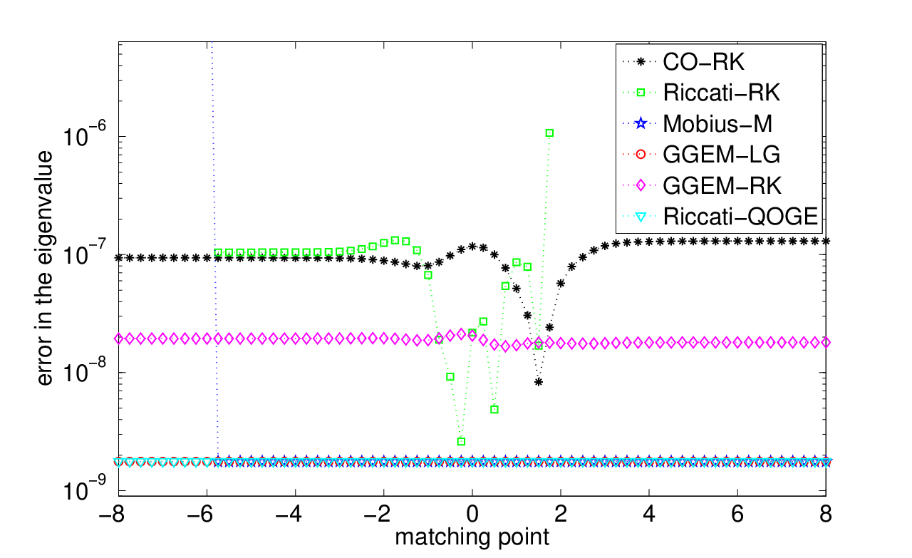
We compare the error in computing the eigenvalue for different choices of matching point—in fact for anywhere in the interval —for all six methods in Figure 7. We see that the most accurate and robust methods are the GGEM-LG and Riccati-QOGE methods. Some methods, such as the Riccati-RK method as discussed already, break down when singularities impinge on the matching point—the singularities in the Evans function are observed in Figure 8. Generally we also see in Figure 7 that the GGEM-LG and Riccati-QOGE methods outperform the CO-RK method in terms of accuracy.
Overall, we observe in this example that when computing the eigenvalue, those methods based on the Magnus expansion are superior in accuracy and efficiency. Note that for GGEM-RK, the quasi-optimal Gaussian elimination process is an additional operation. However, to ensure analyticity for the CO-RK method, there are two additional matrix-matrix multiplications in the equations for (operational cost ) required at each step.
7.3. Autocatalytic fronts
As a second example, we study travelling waves in a model of autocatalysis in an infinitely extended medium
Here is the concentration of the reactant and is the concentration of the autocatalyst. We suppose approaches the stable homogeneous steady state as , and the unstable homogeneous steady state as . The diffusion parameter is the ratio of the diffusivity of the reactant to that of the autocatalyst and is the order of the autocatalytic reaction. The speed of the co-moving reference frame is . The system is globally well-posed for smooth initial data and any finite and .
From Billingham and Needham [9] we know that a unique heteroclinic connection between the unstable and stable homogeneous steady states exists for wavespeeds . The unique travelling wave for converges exponentially to the homogeneous steady states and is computed by a simple shooting algorithm (see Balmforth, Craster and Malham [8]). The resulting travelling wave for and is shown in Figure 9.


The stability of the travelling wave of velocity can be deduced from the location of the spectrum of the eigenvalue problem , where
where and represent the travelling wave solution.
The pulsating instability occurs when is sufficiently small and is sufficiently large (see Metcalf, Merkin and Scott [72] and Balmforth, Craster and Malham [8]). For fixed and increasing, a complex conjugate pair of eigenvalues crosses into the right-half -plane signifying the onset of instability via a Hopf bifurcation. Figure 10 shows the onset of this instability for as is increased from to (see Aparicio, Malham and Oliver [7]). The figure shows the zero contour lines of the real and imaginary parts of the Evans function. Solid lines correspond to zero contours of the real part of , dashed lines to the imaginary part of . We see that a complex-conjugate pair of eigenvalues crosses into the right-half plane, indicating the onset of instability. Figure 10 was constructed using the Riccati-RK method with the fixed coordinate patches identified by from to , and from to . The matching point is chosen roughly centred on the wavefront.


We compare the Riccati-RK, Möbius–Magnus, CO-RK and GGEM-LG methods in Figure 11 where we plot the absolute error in the eigenvalue vs the stepsize (upper panel) and also vs cputime (lower panel). The eigenvalue in question is that in the first quadrant in Figure 10 for and . Figure 11 was generated as follows. Starting with an initial guess lying within a small square around the eigenvalue, we iterated a standard root finding algorithm until we arrived in a square (containing the eigenvalue) which was smaller than a preset tolerance. We see in Figure 11 that the Riccati-RK method produces a slightly better error for a given stepsize, and is marginally more efficient than the GGEM-LG method. The CO-RK method produces a larger error for a given computational effort. This is not surprising, as again, the matrices in the Drury–Oja vector field are twice as big () as the ones in the Riccati vector fields ().
When we match at , there is little to distinguish the Riccati-RK, Möbius–Magnus, CO-RK and GGEM-LG methods. We compare all four methods for different matching positions in Figure 12, which was generated using the same root finding criteria as for Figure 11, except all the methods used steps. Note that the errors in the Möbius–Magnus and GGEM-LG methods are uniform for any matching values in the range . The CO-RK method error doesn’t vary that much either and is slightly larger. Note that no values are plotted for the CO-RK method at the matching points . In these cases the classical Runge–Kutta method applied to the Drury–Oja vector field is unstable for steps for some -values close to the eigenvalue. This problem is resolved by increasing the number of steps to . For a range of matching positions roughly in , there are no singularities of the Riccati-RK method in the left and right-hand integration intervals for values of the spectral parameter close to the eigenvalue. Indeed for this range of matching positions the Riccati-RK method delivers the best accuracy. However for matching positions outside this range, for values of the spectral parameter not far from the eigenvalue, the Riccati-RK solution does have a singularity for some matching points (which we can see in the contour plots in Figure 13). This makes the eigenvalue-searching algorithm fail—indicated by no error points for those matching position values. We also do not show the error for the Riccati-RK method for the matching points , as there are singularities in the Evans function close to the real axis for these matching points (again see Figure 13). This means that we cannot for example, apply the argument principle in the first quadrant, though starting sufficiently close to the eigenvalue we can still use the Riccati-RK method as part of a root-finding algorithm to determine the eigenvalue.


Figure 13 shows the contour lines of for and , close to the eigenvalue in the first quadrant, when using the Riccati-RK, Möbius-Magnus, CO-RK and GGEM-LG methods, respectively, and matching at three positions . We see that the CO-RK and GGEM-LG methods show the least sensitivity to the choice of matching position and produce smooth contour plots for all three matching points. The contour plots across shape and scale look very similar for both these methods. By contrast the Riccati-RK and Möbius-Magnus methods appear to develop singularities close to the eigenvalue when the matching position is or .
Lastly in Figure 14 we demonstrate the argument principle for counting zeros of the Evans function inside closed contours. We computed the Evans function using the GGEM-LG method and matched at . As expected, if the closed contour in the complex -plane encloses the eigenvalue, then the change in the argument of the Evans function around the complete contour is one (once we have accounted for the factor in the argument principle). We also show, for each fixed value, the number of patch changes that occured as we integrated from through to .
7.4. Ekman boundary layer
The third test system is a boundary layer flow over a flat plate which is infinitely extended in the and direction and rotates around the half infinite -axis with a given rotational speed. Linear stability of the Ekman boundary layer has been investigated in Allen and Bridges [6] and Allen [4] using the compound matrix method. The flow is governed by the continuity equation , and the Navier-Stokes equations in a co-rotating frame
Here , and denote the Reynolds, Rossby and Ekman numbers, respectively.
After non-dimensionalization and setting , , the linear stability of the boundary layer is determined by the eigenvalues of the linear problem , where (see Allen [4, p. 176])
and
Here the parameters and represent the radial and angle components, respectively, of a polar coordinate parameterization of horizontal wavenumbers associated with the and directions—see Allen and Bridges [6] for more details.
We choose the fixed coordinate patch identified by to integrate the corresponding Riccati equation from to . The boundary condition for the rigid wall at as given in Allen and Bridges is
If
then the boundary conditions are equivalent to
We thus compute the Evans function:


We computed neutral curves, i.e. curves in the – plane where , using the Riccati-RK method with to compute and consequently the Evans function . For continuation of the curves we used the Matlab package MatCont which uses pseudo-arclength continuation (Dhooge, Govaerts and Kuznetsov [29]). Figures 15 and 16 show the neutral curves which match those in Allen and Bridges [6] and Allen [4]. The integration of the Riccati system has been done with the Matlab ODE-solver ode23s from to (as in Allen and Bridges) with absolute and relative tolerances and . The stable subspace of was constructed using the Matlab eigenvalue-solver eig (we also used direct formulae for the eigenvectors to construct analytic bases for the stable subspace but this did not significantly change the overall performance).
For comparison we also implemented the CO-RK and GGEM-LG methods. We tested the performance of all three methods, in each case evaluating the Evans function on a grid for in the complex plane. In Figures 17 we present contour plots of , and see that all methods find a root at . The computation times for a Ghz machine were: seconds for Riccati-RK, seconds for GGEM-LG and seconds for CO-RK. As a comprehensive check, we also implemented the compound matrix method (i.e. Plücker coordinates, of which there are ), described in Allen and Bridges, for this performance test. As expected, since this method involves integrating a linear system of order , it was an order of magnitude slower (while giving the same results).
8. Concluding discussion
We have shown that the new scaled Grassmann Gaussian elimination method as well as the Riccati method with quasi-optimal patch swapping, compete with the continuous orthogonalization method for computing the Evans function. Both new methods deliver superior accuracy for the same computational cost when combined with Lie group Magnus integration to advance the solution. Moreover, as hoped, numerically these new methods appear to be robust in the sense that they are insensitive to the choice of the matching position in the computational domain. We now outline several directions in which we plan to use and extend these methods.
One of the main goals we have had in mind in this paper is that of large scale spectral problems, in particular the stability of travelling waves with a multi-dimensional structure. There is recent research extending the Evans function approach in this direction—see Deng and Nii [27], Gesztesy, Latushkin and Makarov [36] and Gesztesy, Latushkin and Zumbrun [37]. From a numerical perspective we have, together with Niesen, implemented some of the methods we propose in this paper in a multi-dimensional context. In particular, it is well known in autocatalysis and combustion that planar travelling fronts can be unstable to transverse perturbations and develop into steadily propagating travelling fronts with wrinkles. In Ledoux, Malham, Niesen and Thümmler [66] we show that the wrinkled fronts themselves develop an instability as a diffusion parameter is further increased.
For large scale problems the Lie group methods we propose using the Magnus expansion may become prohibitive. This is because of the effort required to compute the matrix exponential—see Moler and Van Loan [75], Celledoni and Iserles [19], Munthe-Kaas and Zanna [78] and Iserles and Zanna [53]. For the examples we considered this was not an issue. However it remains to be seen if such Lie group methods will be cost effective for larger problems—the methods we proposed based on Runge–Kutta integration such as GGEM-RK can be used as they scale favourably with system size.
The constructs and Grassmannian reductions we have considered in this paper, it turns out, have their origins in the control theory literature dating back to the early seventies, in particular in the pioneering papers of Hermann and Martin [44, 45, 46, 47, 48], Martin and Hermann [71] and Brockett and Byrnes [18]. We also found Bittanti, Laub and Willems [12], Lafortune and Winternitz [63], Rosenthal [87], Shayman [92] and Zelikin [100] particularly useful resources. A future direction we would like to explore is whether there are any applications of the numerical methods we have outlined here to practical non-autonomous control problems?
Riccati methods in particular also have their origins in the quantum chemistry literature also dating back to the early seventies—a recent survey of these numerical methods can be found in Chou and Wyatt [24]. However also see Light and Walker [67], Johnson [56], Hutson [51] and Gray and Manopoulous [39]. In particular the log-derivative and -propagation methods correspond to special choices of Grassmannian patch in the Riccati methods we mention above. Prüfer methods, for which we can think of the patch evolving, originate even further back; see Prüfer [84] and Pryce [85].
Of course, our quasi-optimal Gaussian elimination process for choosing a suitable representative patch was inspired by the Schubert cell decomposition of the Grassmann manifold; see for example Billey [10], Griffiths and Harris [40], Kleiman and Laksov [58], Kresch [60], Postnikov [83], Sottile [93] and, in a somewhat different vein, Kodama [59]. Since the Grassmann manifold is the disjoint union of Schubert cells, the question is, can we express the flow on the Grassmann manifold as a flow on Schubert cells (see Griffiths and Harris and also Ravi, Rosenthal and Wang [86])? Can we construct the corresponding flow on the cohomological ring of Schubert cycles (Chern [22]; Fulton [35])?
Acknowledgements
We would especially like to thank the anonymous referee #2, who coined the following phrase for the Riccati flow in an earlier version of this manuscript: this approach is more of Gaussian elimination type (including the question of pivoting, which is not discussed here). This comment eventually lead us to the Grassmann Gaussian elimination method we investigate in this paper. We also thank this referee for pointing out our incomplete analyticity arguments in the second draft. We would also like to thank referee #1 for useful background on the history of the Evans function, and referee #3 for making us aware of the control theory literature associated with this topic. Chris Jones, Yuri Latushkin, Bob Pego, Bjorn Sandstede and Arnd Scheel organised a workshop at AIM in Palo Alto in May 2005 on Stability Criteria for Multi-Dimensional Waves and Patterns, which instigated the topic of this paper. All three authors were visiting the Isaac Newton Institute in the Spring of 2007 when this research was initiated. We would like to thank Arieh Iserles and Ernst Hairer for inviting us and providing so much support and enthusiasm. We are also indebted to the facilities at the Isaac Newton Institute which were invaluable. We also thank Tom Bridges, Jitse Niesen, Jacques Vanneste and Antonella Zanna for stimulating discussions on this work. Veerle Ledoux is a postdoctoral fellow of the Fund of Scientific Research—Flanders (F.W.O.—Vlaanderen). Vera Thümmler was supported by CRC 701: Spectral Structures and Topological Methods in Mathematics.
References
- [1] H. Abou–Kandil, G. Freiling, V. Ionescu and G. Jank, Matrix Riccati equations in control and systems theory, Systems and control: Foundations and applications, Birkhäuser, 2003.
- [2] J.C., Alexander, R. Gardner, and C.K.R.T. Jones, A topological invariant arising in the stability analysis of traveling waves, J. Reine Angew. Math. 410 (1990), pp. 167–212.
- [3] J.C. Alexander and R. Sachs, Linear stability of solitary waves of a Boussinesq-type equation: a computer assisted computation, preprint 30 Apr, 1999.
- [4] L. Allen, Modelling dolphin hydrodynamics: The numerical analysis and hydrodynamic stability of flow past compliant surfaces, PhD Thesis, University of Surrey, 2001.
- [5] L. Allen and T.J. Bridges, Numerical exterior algebra and the compound matrix method, Numer. Math. 92(2) (2002), pp. 131–149.
- [6] L. Allen and T.J. Bridges, Hydrodynamic stability of the Ekman boundary layer including interaction with a compliant surface: a numerical framework, Eur. J. Mech. B Fluids, 22(3) (2003), pp. 239–358.
- [7] N.D. Aparicio, S.J.A. Malham and M. Oliver, Numerical evaluation of the Evans function by Magnus integration, BIT 45 (2005), pp. 219–258.
- [8] N.J. Balmforth, R.V. Craster and S.J.A. Malham, Unsteady fronts in an autocatalytic system, Proc. R. Soc. Lond A. 455 (1999), pp. 1401–1433.
- [9] J. Billingham and D. Needham, The development of travelling waves in quadratic and cubic autocatalysis with unequal diffusion rates, I and II, Phil. Trans. R. Soc. Lond. A, 334 (1991), pp. 1–124, and 336 (1991), pp. 497–539.
- [10] S. Billey, Grassmannians and other Schubert varieties, talk, April 14, 2007.
- [11] D.S. Bindel, J. Demmel and M. Friedman, Continuation of invariant subspaces for large bifurcation problems, SIAM J. Sci. Comp. 30(2) (2008), pp. 637–656.
- [12] S. Bittanti, A.J. Laub and J.C. Willems (Eds.), The Riccati equation, Springer–Verlag, 1991.
- [13] Å. Björck and G.H. Golub, Numerical methods for computing angles between linear subspaces, Math. Comp. 27(123) (1973), pp. 579–594.
- [14] T.J. Bridges, G. Derks and G. Gottwald, Stability and instability of solitary waves of the fifth-order KdV equation: a numerical framework, Physica D 172(1–4) (2002), pp. 190–216.
- [15] T.J. Bridges and S. Reich, Computing Lyapunov exponents on a Stiefel manifold, Physica D 156 (3–4) (2001), pp. 213–238.
- [16] L.Q. Brin, Numerical testing of the stability of viscous shock waves, PhD Thesis, Indiana University, Bloomington, 1998.
- [17] L.Q. Brin, Numerical testing of the stability of viscous schock waves, Math. of Comput. 70(235) (2000), pp. 1071–1088.
- [18] R.W. Brockett and C.I. Byrnes, Multivariable Nyquist criteria, root loci, and pole placement: a geometric viewpoint, IEEE Trans. Automat. control 26(1) (1981), pp. 271–284.
- [19] E. Celledoni and A. Iserles, Approximating the exponential from a Lie algebra to a Lie group, Math. Comp. 69 (2000), pp. 1457–1480.
- [20] E. Celledoni and B. Owren, On the implementation of Lie group methods on the Stiefel manifold, Numer. Algorithms 32 (2003), pp. 163–183.
- [21] H.-C. Chang, E.A. Demekhin and D.I. Kopelevich, Local stability theory of solitary pulses in an active medium, Physica D 97 (1996), pp. 353–375.
- [22] S.S. Chern, Complex manifolds without potential theory, Van Nostrand Mathematical Studies #15, 1967.
- [23] C.–C. Chou and R.E. Wyatt, Computational method for the quantum Hamilton–Jacobi equation: Bound states in one dimension, J. Chem. Phys. 125(174103) (2006), pp. 1–10.
- [24] C.–C. Chou and R.E. Wyatt, Riccati differential equation for qunatum mechanical bound states: comparison of numerical integrators, Int. J. Quant. Chem. 108 (2008), pp.238–248.
- [25] S. Coombes and M. R. Owen, Evans function for integral neural field equations with heaviside firing rate function, submitted to SIAM J. Appl. Dyn. Syst. (2004).’
- [26] I. Coskun, Grassmannians: the first example of a moduli space, MITOpenCourseWare available at http://ocw.mit.edu/NR/rdonlyres/Mathematics/18-727Spring-2006.
- [27] J. Deng and S. Nii, Infinite-dimensional Evans function theory for elliptic eigenvalue problems in a channel, J. Differential Equations 225 (2006), pp. 57–89.
- [28] G. Derks, U. Ebert and B. Meulenbroek, Laplacian instability of planar streamer ionization fronts - an example of pulled front analysis, Journal Nonl. Science, 2008.
- [29] A. Dhooge, W. Govaerts and Y.A. Kuznetsov, MATCONT: a MATLAB package for numerical bifurcation analysis of ODEs, ACM Trans. Math. Software, 29(2) (2003), pp. 141–164.
- [30] L. Dieci and E.S. Van Vleck, Orthonormal integrators based on Householder and Givens transformations, Future Generation Computer Systems 19(3) (2003) Special issue: Geometric numerical algorithms, pp. 363–373.
- [31] A. Doelman, R.A. Gardner and T.J. Kaper, Stability analysis of singular patterns in the 1D Gray-Scott model: A matched asymptotics approach, Physica D 122 (1998), pp. 1–36.
- [32] L.O. Drury, Numerical solution of Orr-Sommerfeld-type equations, J. Comput. Phys. 37(1) (1980), pp. 133–139.
- [33] A. Edelman, T.A. Arias and S.T. Smith, The geometry of algorithms with orthogonality constraints, SIAM. J. Matrix Anal. Appl. 20(2) (1998), pp. 303–353.
- [34] J.W. Evans, Nerve axon equations, IV: The stable and unstable impulse, Indiana Univ. Math. J. 24 (1975), pp. 1169–1190.
- [35] W. Fulton, Young tableaux, London Mathematical Society Student Texts 35, Cambridge University Press, 1997.
- [36] F. Gesztesy, Y. Latushkin and K.A. Makarov, Evans functions, Jost functions, and Fredholm determinants, Arch. Rational Mech. Anal. 186 (2007), pp. 361–421.
- [37] F. Gesztesy, Y. Latushkin and K. Zumbrun, Derivatives of (modified) Fredholm determinants and stability of standing and travelling waves, arXiv:0802.1665v1, 12 Feb 2008.
- [38] S.K. Gray and D.E. Manopoulous, Symplectic integrators tailored to the time-dependent Schrödinger equation, J. Chem. Phys. 104(18) (1996), pp. 7099–7112.
- [39] J. Greenberg and M. Marletta, Numerical solution of non-self-adjoint Sturm-Liouville problems and related systems, SIAM J. Numer. Anal. 38(6) (2000), pp. 1800–1845.
- [40] P. Griffiths and J. Harris, Principles of algebraic geometry, Wiley Classics Library Edition, 1994.
- [41] V. Gubernov, G.N. Mercer, H.S. Sidhu and R.O. Weber, Evans function stability of non-adiabatic combustion waves, Proc. R. Soc. Lond. A 460 (2004), pp. 2415–2435.
- [42] E. Hairer, C. Lubich and G. Wanner, Geometric Numerical Integration, Springer Series in Computational Mathematics, 2002.
- [43] D. Henry, Geometric theory of semilinear parabolic equations, Lecture Notes in Mathematics 840, Springer–Verlag, 1981.
- [44] R. Hermann and C. Martin, Applications of Algebraic geometry to systems theory – part I, IEEE Trans. Automat. Control 22(1) (1977), pp. 19–25.
- [45] R. Hermann and C. Martin, Lie theoretic aspects of the Riccati equation, NASA Report WP2-3:30.
- [46] R. Hermann and C. Martin, Periodic solutions of the Riccati equation, NASA Report TP3-3:00, IEEE (1980).
- [47] R. Hermann and C. Martin, Lie and Morse theory for periodic orbits of vector fields and matrix Riccati equations, I: General Lie-theoretic methods, Mathematical Systems Theory 15 (1982), pp. 277–284.
- [48] R. Hermann and C. Martin, Lie and Morse theory for periodic orbits of vector fields and matrix Riccati equations, II, Mathematical Systems Theory 16 (1983), pp. 297–306.
- [49] J. Humpherys and K. Zumbrun, An efficient shooting algorithm for Evans function calculations in large systems, Physica D 220 (2006), pp. 116–126.
- [50] J. Humpherys, B. Sandstede and K. Zumbrun, Efficient Computation of Analytic Bases in Evans Function Analysis of Large Systems, Numer. Math. 103(4) (2006), pp. 631-642.
- [51] J.M. Hutson, Coupled channel methods for solving the bound-state Schrödinger equation, Computer Physics Communications 84 (1994), pp. 1–18.
- [52] A. Iserles, A. Marthinsen and S.P. Nørsett, On the impementation of the method of Magnus series for linear differential equations, BIT 39(2) (1999), pp. 281–304.
- [53] A. Iserles and A. Zanna, Efficient computation of the matrix exponential by generalized polar decompositions, SIAM J. Numer. Anal. 42(5) (2005), pp. 2218–2256.
- [54] A. Iserles, H. Z. Munthe-Kaas, S. P. Nørsett, and A. Zanna, Lie-group methods, Acta Numer. (2000), pp. 215–365.
- [55] L.Gr. Ixaru, Special techniques related to the CP methods for the coupled channel Schrödinger equation, talk given at Workshop Numerical Approach of Oscillatory functions 2008, Ghent.
- [56] B.R. Johnson, New numerical methods applied to solving the one-dimensional eigenvalue problem, J. Chem. Phys. 67(9) (1977), pp. 4086–4093.
- [57] T. Kapitula and B. Sandstede, A novel instability mechanism for bright solitary-wave solutions to the cubic-quintic Ginzburg–Landau equation, J. Opt. Soc. Amer. B 15 (1998), pp. 2757–2762.
- [58] S.L. Kleiman and D. Laksov, Schubert calculus, Amer. Math. Month. 79(10) (1972), pp. 1061–1082.
- [59] Y. Kodama, Young diagrams and -soliton solutions of the KP equation, J. Phys. A: Math. Gen. 37 (2004), pp. 11169–11190.
- [60] A. Kresch, Flag varieties and Schubert calculus, preprint, July 2005.
- [61] S. Krogstad, A low complexity Lie group method on the Stiefel manifold, Reports in Informatics, ISSN 0333-3590, 2001.
- [62] S. Lafortune and J. Lega, Instability of local deformations of an elastic rod, Physica D 182 (2003), pp. 103–124.
- [63] S. Lafortune and P. Winternitz, Superposition formulas for pseudounitary Riccati equations, J. Math. Phys. 37 (1996). pp. 1539-1550.
- [64] V. Ledoux, Study of special algorithms for solving Sturm-Liouville and Schrödinger equations. PhD Thesis, Universiteit Gent, 2007.
- [65] V. Ledoux, M. Van Daele and G. Vanden Berghe, A numerical procedure to solve the multichannel Schrödinger eigenvalue problem, Comp. Phys. Commun. 176 (2007). pp. 191-199.
- [66] V. Ledoux, S.J.A. Malham, J. Niesen and V. Thümmler, Computing stability of multi-dimensional travelling waves, SIADS 8(1) (2009), pp. 480–507.
- [67] J.C. Light and R.B. Walker, An R matrix approach to the solution of coupled equations for atom-molecule reactive scattering, J. Chem. Phys. 65(10) (1976), p. 4272–4282.
- [68] W. Magnus, On the exponential solution of differential equations for a linear operator, Comm. Pure Appl. Math., 7 (1954), pp. 649–673.
- [69] D.E. Manopoulous and S.K. Gray, Symplectic integrators for the multichannel Schrödinger equation, J. Chem. Phys. 102(23) (1995), pp. 9214–9227.
- [70] J. E. Marsden and T. S. Ratiu, Introduction to mechanics and symmetry, Second edition, Springer, 1999.
- [71] C. Martin and R. Hermann, Applications of algebraic geometry to systems theory: The McMillan degree and Kronecker indicies of transfer functions as topological and holomorphic system invariants, SIAM J. Control Optim. 16(5) (1978), pp. 743–755.
- [72] M.J. Metcalf, J.H. Merkin and S.K. Scott, Oscillating wave fronts in isothermal chemical systems with arbitrary powers of autocatalysis, Proc. R. Soc. Lond. A 447 (1994), pp. 155-174.
- [73] C. Meyer, Matrix analysis and applied linear algebra, SIAM, 2000.
- [74] J.W. Milnor and J.D. Stasheff, Characteristic classes, Annals of mathematics studies 76, Princeton University Press, 1974.
- [75] C. Moler and C. Van Loan, Nineteen dubious ways to compute the exponential of a matrix, twenty-five years later, SIAM Rev. 45 (2003), pp. 3–49.
- [76] R. Montgomery, A tour of subRiemannian geometries, their geodesics and applications, Mathematical Surveys and Monographs 91, American Mathematical Society, 2002.
- [77] H. Munthe-Kaas, High order Runge–Kutta methods on manifolds, Appl. Numer. Math., 29 (1999), pp. 115–127.
- [78] H. Munthe-Kaas and A. Zanna, Generalized polar decompositions for the approximation of the matrix exponential, SIAM J. Matrix Anal. Applic. 23(3) (2002), pp. 840–862.
- [79] S. Nii, An extension of the stability index for traveling-wave solutions and its application to bifurcations, SIAM J. Math. Anal. 28(2) (1997), pp. 402–433.
- [80] E. Oja, A Simplified Neuron Model as a Principal Component Analyzer, J. Math. Biology 15 (1982), pp. 267–273.
- [81] P.J. Olver, Equivalence, Invariants, and symmetry, Cambridge University Press, 1995.
- [82] R.L. Pego and M.I. Weinstein, Eigenvalues and instabilities of solitary waves, Phil. Trans. R. Soc. Lond. A 340 (1992), pp. 47–94.
- [83] A. Postnikov, Total positivity, Grassmannians, and Networks, arXiv:math/060976v1 27 Sep 2006.
- [84] H. Prüfer, Neue Herleitung der Sturm–Liouvilleschen Reihenentwicklung, Math. Ann. 95 (1923), pp. 499–518.
- [85] J.D. Pryce, Numerical solution of Sturm–Liouville problems, Monographs of Numerical Analysis, Oxford Science Publications, Clarendon Press, 1993.
- [86] M.S. Ravi, J. Rosenthal and X. Wang, Dynamic pole assignment and Schubert calculus, SIAM J. Control Optim. 34(3) (1996), pp. 813–832.
- [87] J. Rosenthal, The Hermann–Martin curve, preprint report.
- [88] B. Sandstede, Stability of travelling waves, In Handbook of Dynamical Systems II, B. Fiedler, ed., Elsevier (2002), pp. 983–1055.
- [89] B. Sandstede and A. Scheel, Curvature effects on spiral spectra: Generation of point eigenvalues near branch points, Phys. Rev. E 73 106217, 2006.
- [90] J. Schiff and S. Shnider, A natural approach to the numerical integration of Riccati differential equations, SIAM J. Numer. Anal. 36(5) (1999), pp. 1392–1413.
- [91] C.R. Schneider, Global aspects of the matrix Riccati equation, Theory of Computing Systems 7(3) (1973), pp. 281–286.
- [92] M.A. Shayman, Phase portrait of the matrix Riccati equation, SIAM J. Control Optim. 24(1) (1986), pp. 1–65.
- [93] F. Sottile, Rational curves on Grassmannians: systems theory, reality, and transversality, In “Advances in Algebraic Geometry Motivated by Physics”, ed. by Emma Previato, Contemporary Mathematics 276 (2001), pp. 9–42.
- [94] N. Steenrod, The topology of fibre bundles, Princeton University Press, 1951.
- [95] J. Swinton and J. Elgin, Stability of travelling pulse solutions to a laser equation, Phys. Lett. A 145(8–9) (1990), pp.428–433.
- [96] D. Terman, Stability of planar wave solutions to a combustion model, SIAM J. Math. Anal., 21 (1990), pp. 1139–1171.
- [97] F.W. Warner, Foundations of differentiable manifolds and Lie groups, Graduate texts in mathematics, Springer, 1983.
- [98] W-Y. Yan, U. Helmke and J.B. Moore, Global analysis of Oja’s flow for neural networks, IEEE Transactions on Neural Networks 5(5) (1994), pp. 674–683.
- [99] X. Ying and I. Katz, A reliable argument principle algorithm to find the number of zeros of an analytic function in a bounded domain, Numer. Math. 53 (1988), pp. 143–163.
- [100] M.I. Zelikin, Control theory and optimization I: Homogeneous spaces and the Riccati equation in the calculus of variations, Encyclopaedia of Mathematical Sciences, Volume 86, Springer–Verlag 2000.