Self-consistent quasiparticle RPA for multi-level pairing model

N. Quang Hung¹ On leave of absence from the Institute of Physics and Electronics, Hanoi, Vietnam Email: nqhung@riken.jp N. Dinh Dang^1,2 Email: dang@riken.jp Affiliation: ¹ Heavy-Ion Nuclear Physics Laboratory, RIKEN Nishina Center for Accelerator-Based Science, 2-1 Hirosawa, Wako City, 351-0198 Saitama, Japan
² Institute for Nuclear Science and Technique, Vietnam Atomic Energy Commission, Hanoi, Vietnam

August 11, 2026

Abstract

Particle-number projection within the Lipkin-Nogami (LN) method is applied to the self-consistent quasiparticle random-phase approximation (SCQRPA), which is tested in an exactly solvable multi-level pairing model. The SCQRPA equations are numerically solved to find the energies of the ground and excited states at various numbers $\Omega$ of doubly degenerate equidistant levels. The use of the LN method allows one to avoid the collapse of the BCS (QRPA) to obtain the energies of the ground and excited states as smooth functions of the interaction parameter $G$ . The comparison between results given by different approximations such as the SCRPA, QRPA, LNQRPA, SCQRPA and LNSCQRPA is carried out. While the use of the LN method significantly improves the agreement with the exact results in the intermediate coupling region, we found that in the strong coupling region the SCQRPA results are closest to the exact ones.

Keywords:

Suggested keywords

pacs

21.60.Jz, 21.60.-n

I INTRODUCTION

The random-phase approximation (RPA), which includes correlations in the ground state, provides a simple theory of excited states of the nucleus. However, the RPA breaks down at a certain value $G_{\rm cr}$ of interaction parameter $G$ , where it yields imaginary eigenvalues. The reason is that the RPA equations, linear with respect to the $X$ and $Y$ amplitudes of the RPA excitation operator, are derived based on the quasi-boson approximation (QBA). The latter neglects the Pauli principle between fermion pairs and its validity is getting poor with increasing the interaction parameter $G$ . The collapse of the RPA at the critical value $G_{\rm cr}$ of $G$ invalidates the use of the QBA. The RPA therefore needs to be extended to correct this deficiency, at least for finite systems such as nuclei.
One of methods to restore the Pauli principle is to renormalize the conventional RPA to include the non-zero values of the commutator between the fermion-pair operators in the correlated ground state. These so-called ground-state correlations beyond RPA are neglected within the QBA. The interaction in this way is renormalized and the collapse of RPA is avoided. The resulting theory is called the renormalized RPA (RRPA) RRPA1; Rowe; RRPA5. However, the test of the RRPA carried out within several exactly solvable models showed that the RRPA results are still far from the exact solutions RRPA5; SCRPA1; SCRPA2.
Recently, a significant development in improving the RPA has been carried out within the self-consistent RPA (SCRPA) SCRPA1; SCRPA2; SCRPA3. Based on the same concept of renormalizing the particle-particle ( $pp$ ) RPA, the SCRPA made a step forward by including the screening factors, which are the expectation values of the products of two pairing operators in the correlated ground state. The SCRPA has been applied to the exactly solvable multi-level pairing model, where the energies of the ground state and first excited state in the system with $N+2$ particles relative to the energy of the ground-state level in the $N$ -particle system are calculated and compared with the exact results. It has been found that the agreement with the exact solutions is good only in the weak coupling region, where the pairing-interaction parameter $G$ is smaller than the critical values $G_{\rm cr}$ . In the strong coupling region ( $G>>G_{\rm cr}$ ), the agreement between the SCRPA and exact results becomes poor SCRPA1; SCRPA2. In this region a quasiparticle representation should be used in place of the $pp$ one, as has been pointed out in Ref. DaTa. As a matter of fact, an extended version of the SCRPA in the superfluid region has been proposed and is called the self-consistent quasiparticle RPA (SCQRPA), which was applied for the first time to the seniority model in Ref. SCQRPA1 and a two-level pairing model in Ref. SCQRPA2. However, the SCQRPA also collapses at $G=G_{\rm cr}$ . It is therefore highly desirable to develop a SCQRPA that works at all values of $G$ and also in more realistic cases, e.g. multi-level models. The aim of the present work is to construct such an approach. Obviously, the collapse of the SCQRPA at $G=G_{\rm cr}$ , which is the same as that of the non-trivial solution for the pairing gap within the Bardeen-Cooper-Schrieffer theory (BCS), can be removed by performing the particle-number projection (PNP). The Lipkin-Nogami method Lipkin; Nogami5, which is an approximated PNP before variation, will be used in such extension of the SCQRPA in the present paper because of its simplicity. This approach shall be applied to a multi-level pairing model, the so-called Richardson model Richardson-model, which is an exactly solvable model extensively employed in literature to test approximations of many-body problems.
The paper is organized as follows. Section II presents a brief outline of the SCQRPA theory that includes the PNP within the LN method. The results of numerical calculations are analyzed and discussed in sec. III. Conclusions are drawn in the last section.

II FORMALISM

II.1 Model Hamiltonian

The Richardson model (also called the multi-level pairing model, picket-fence model or ladder model, etc) was described in detail in Refs. Richardson-model; SCRPA1; SCRPA2; SCRPA3. It consists of $\Omega$ doubly-fold equidistant levels interacting via a pairing force with a constant parameter $G$ . The model Hamiltonian is given as

H=\sum_{j=1}^{\Omega}(\epsilon_{j}-\lambda)N_{j}-G\sum_{j,j^{\prime}=1}^{\Omega}{P_{j}^{\dagger}P_{j^{\prime}}}~,

(1)

where $\epsilon_{j}$ are the single-particle energies on the j-shells. The particle-number operator $N_{j}$ and pairing operators $P_{j}^{\dagger}$ , $P_{j}$ on the $j$ -th orbital (with unit shell degeneracy $j+1/2\equiv 1$ ) are defined as

	$\displaystyle N_{j}=a_{j}^{\dagger}a_{j}+a_{-j}^{\dagger}a_{-j}~,$		(2)
	$\displaystyle P_{j}^{\dagger}=a_{j}^{\dagger}a_{-j}^{\dagger}~,\hskip 14.22636ptP_{j}=(P_{j}^{\dagger})^{\dagger}~.$		(3)

These operators fulfill the following exact commutation relations

	$\displaystyle[P_{j}~,~P_{j^{\prime}}^{\dagger}]=\delta_{jj^{\prime}}(1-N_{j})~,$		(4)
	$\displaystyle[N_{j}~,~P_{j^{\prime}}^{\dagger}]=2\delta_{jj^{\prime}}P_{j^{\prime}}^{\dagger}~,\hskip 14.22636pt[N_{j}~,~P_{j^{\prime}}]=-2\delta_{jj^{\prime}}P_{j^{\prime}}~.$		(5)

By using the Bogoliubov transformation from particle operators $a_{j}^{\dagger}$ and $a_{j}$ to quasiparticle ones $\alpha_{j}^{\dagger}$ and $\alpha_{j}$

a_{j}^{\dagger}=u_{j}\alpha_{j}^{\dagger}+v_{j}\alpha_{-j}~,\hskip 14.22636pta_{-j}=u_{j}\alpha_{-j}-v_{j}\alpha_{j}^{\dagger}~,

(6)

the pairing Hamiltonian in Eq. (1) is transformed into the quasiparticle Hamiltonian as quasi-ha1; quasi-ha2

H=a+\sum_{j}{b_{j}\mathcal{N}_{j}}+\sum_{j}{c_{j}(\mathcal{A}_{j}^{\dagger}+\mathcal{A}_{j}})+\sum_{jj^{\prime}}{d_{jj^{\prime}}\mathcal{A}_{j}^{\dagger}\mathcal{A}_{j^{\prime}}}+\sum_{jj^{\prime}}{g_{j}(j^{\prime})(\mathcal{A}_{j^{\prime}}^{\dagger}\mathcal{N}_{j}+\mathcal{N}_{j}\mathcal{A}_{j^{\prime}})}

+\sum_{jj^{\prime}}{h_{jj^{\prime}}(\mathcal{A}_{j}^{\dagger}\mathcal{A}_{j^{\prime}}^{\dagger}+\mathcal{A}_{j^{\prime}}\mathcal{A}_{j})}+\sum_{jj^{\prime}}{q_{jj^{\prime}}\mathcal{N}_{j}\mathcal{N}_{j^{\prime}}}~,

(7)

where $\mathcal{N}_{j}$ is the quasiparticle-number operator, while $\mathcal{A}_{j}^{\dagger}$ and $\mathcal{A}_{j}$ are the creation and destruction operators of a pair of time-conjugated quasiparticles:

	$\displaystyle\mathcal{N}_{j}=\alpha_{j}^{\dagger}\alpha_{j}+\alpha_{-j}^{\dagger}\alpha_{-j}~,$		(8)
	$\displaystyle\mathcal{A}_{j}^{\dagger}=\alpha_{j}^{\dagger}\alpha_{-j}^{\dagger}~,\hskip 14.22636pt\mathcal{A}_{j}=(\mathcal{A}_{j}^{\dagger})^{\dagger}~.$		(9)

The commutation relations between operators $\mathcal{N}_{j}$ , $\mathcal{A}_{j}^{\dagger}$ and $\mathcal{A}_{j}$ are similar to those for particle operators in Eqs. (4) and (5), namely

	$\displaystyle[\mathcal{A}_{j}~,~\mathcal{A}_{j^{\prime}}^{\dagger}]=\delta_{jj^{\prime}}(1-\mathcal{N}_{j})~,$		(10)
	$\displaystyle[\mathcal{N}_{j}~,~\mathcal{A}_{j^{\prime}}^{\dagger}]=2\delta_{jj^{\prime}}\mathcal{A}_{j^{\prime}}^{\dagger}~,\hskip 14.22636pt[\mathcal{N}_{j}~,~\mathcal{A}_{j^{\prime}}]=-2\delta_{jj^{\prime}}\mathcal{A}_{j^{\prime}}~.$		(11)

The coefficients $a$ , $b_{j}$ , $c_{j}$ , $d_{jj^{\prime}}$ , $g_{j}(j^{\prime})$ , $h_{jj^{\prime}}$ , $q_{jj^{\prime}}$ in Eq. (7) are given in terms of the coefficients $u_{j}$ , $v_{j}$ of the Bogoliubov transformation, and the single particle energies $\epsilon_{j}$ as (see, e.g. Ref. quasi-ha1; quasi-ha2)

a=2\sum_{j}{(\epsilon_{j}-\lambda)v_{j}^{2}}-G\left(\sum_{j}{u_{j}v_{j}}\right)^{2}-G\sum_{j}{v_{j}^{4}}~,

(12)

b_{j}=(\epsilon_{j}-\lambda)(u_{j}^{2}-v_{j}^{2})+2Gu_{j}v_{j}\sum_{j^{\prime}}{u_{j^{\prime}}v_{j^{\prime}}}+Gv_{j}^{4}~,

(13)

c_{j}=2(\epsilon_{j}-\lambda)u_{j}v_{j}-G(u_{j}^{2}-v_{j}^{2})\sum_{j^{\prime}}{u_{j^{\prime}}v_{j^{\prime}}}-2Gu_{j}v_{j}^{3}~,

(14)

d_{jj^{\prime}}=-G(u_{j}^{2}u_{j^{\prime}}^{2}+v_{j}^{2}v_{j^{\prime}}^{2})=d_{j^{\prime}j}~,

(15)

g_{j}(j^{\prime})=Gu_{j}v_{j}(u_{j^{\prime}}^{2}-v_{j^{\prime}}^{2})~,

(16)

h_{jj^{\prime}}=\frac{G}{2}(u_{j}^{2}v_{j^{\prime}}^{2}+v_{j}^{2}u_{j^{\prime}}^{2})=h_{j^{\prime}j}~,

(17)

q_{jj^{\prime}}=-Gu_{j}v_{j}u_{j^{\prime}}v_{j^{\prime}}=q_{j^{\prime}j}~.

(18)

The single-particle energies are given as $\epsilon_{j}=j\epsilon$ , where $j=$ 1, $\dots$ , $\Omega$ , and $\epsilon$ is the level distance chosen to be equal to 1 MeV in the present work. The chemical potential $\lambda$ and the coefficients $u_{j}$ and $v_{j}$ are determined by solving the gap equations discussed in the next section.

II.2 Gap and number equations

II.2.1 Renormalized BCS

It is well known that the Pauli principle between the quasiparticle-pair operators $\mathcal{A}_{j}$ and $\mathcal{A}_{j^{\prime}}^{\dagger}$ is neglected within the conventional BCS, which assumes that $\langle{\rm BCS}|{\cal N}_{j}|{\rm BCS}\rangle=$ 0 within the BCS ground state $|{\rm BCS}\rangle$ . A simple way to restore the Pauli principle is to introduce a new ground state $|\bar{0}\rangle$ in which the correlations among quasiparticles lead to nonzero values of the quasiparticle occupation numbers so that the contribution of the $\mathcal{N}_{j}$ -term at the right-hand side (rhs) of Eq. (10) is preserved. By doing so, the BCS equations are renormalized and the resulting theory is called the renormalized BCS (RBCS) RBCS. Within the RBCS the commutator between the quasiparticle-pair operators are defined as

\langle\bar{0}|[\mathcal{A}_{j},\mathcal{A}_{j^{\prime}}^{\dagger}]|\bar{0}\rangle=\delta_{jj^{\prime}}\langle{\cal D}_{j}\rangle~,

(19)

with

{\cal D}_{j}=1-{\cal N}_{j}~,\hskip 14.22636pt\langle{\cal D}_{j}\rangle=1-2n_{j}~,

(20)

where $n_{j}$ is the quasiparticle number in the correlated ground state $|\bar{0}\rangle$

n_{j}\equiv\frac{1}{2}\langle\bar{0}|\mathcal{N}_{j}|\bar{0}\rangle\neq 0~.

(21)

Taking into account Eq. (19) and performing a constrained variational calculation to minimize the Hamiltonian $H\equiv H^{\prime}-\lambda\hat{N}$ , where $\hat{N}=\sum_{j}N_{j}$ is the particle-number operator, the RBCS equations for the pairing gap $\Delta$ and particle number $N$ have been derived as RBCS

{\Delta}=G\sum_{j}\tau_{j}~,\hskip 5.69054ptN=2\sum_{j}\rho_{j}~,

(22)

where

\tau_{j}=u_{j}v_{j}\langle{\cal D}_{j}\rangle~,\hskip 14.22636pt\rho_{j}=v_{j}^{2}\langle{\cal D}_{j}\rangle+\frac{1}{2}(1-\langle{\cal D}_{j}\rangle)~,

(23)

u_{j}^{2}=\frac{1}{2}\left(1+\frac{\epsilon_{j}-Gv_{j}^{2}-\lambda}{E_{j}}\right)~,\hskip 14.22636ptv_{j}^{2}=\frac{1}{2}\left(1-\frac{\epsilon_{j}-Gv_{j}^{2}-\lambda}{E_{j}}\right)~,

(24)

{E}_{j}=\sqrt{(\epsilon_{j}-Gv_{j}^{2}-\lambda)^{2}+{\Delta}^{2}}~.

(25)

The renormalization factors $\langle{\cal D}_{j}\rangle$ , called the ground-state correlation factors, are obtained by solving the SCQRPA equations discussed later in this paper (See Sec. II.4.2). The internal energy of the system within the RBCS ground state (the RBCS ground-state energy) is given as

E_{\rm g.s.}^{\rm RBCS}=2\sum_{j}(\epsilon_{j}-\lambda){\rho}_{j}-\frac{{\Delta}^{2}}{G}-G\sum_{j}{\rho}_{j}^{2}~.

(26)

By setting $\langle{\cal D}_{j}\rangle=1$ , the RBCS equations go back to the well-known BCS ones.

II.2.2 BCS with SCQRPA correlations

In the minimization procedure, which leads to the equation (See, e.g. Ref. DukSchu)

\langle\bar{0}|[H,{\cal A}_{j}^{\dagger}]|\bar{0}\rangle=0~,

(27)

the RBCS ignores the expectation values $\langle\mathcal{A}_{j^{\prime}}^{\dagger}\mathcal{A}_{j}\rangle\equiv\langle\bar{0}|\mathcal{A}_{j^{\prime}}^{\dagger}\mathcal{A}_{j}|\bar{0}\rangle$ and $\langle\mathcal{A}_{j^{\prime}}\mathcal{A}_{j}\rangle\equiv\langle\bar{0}|\mathcal{A}_{j^{\prime}}\mathcal{A}_{j}|\bar{0}\rangle$ of the products of pair operators in the correlated quasiparticle ground state $|\bar{0}\rangle$ . By retaining these screening factors in calculating the left-hand side (lhs) of Eq. (27), we derive from Eq. (27) an equation for the level-dependent pairing gap in the form

\Delta_{j}=G\frac{\sum_{j^{\prime}}u_{j^{\prime}}v_{j^{\prime}}\langle{\cal D}_{j}{\cal D}_{j^{\prime}}\rangle}{\langle{\cal D}_{j}\rangle}~,

(28)

with the single-particle energies $\epsilon_{j}$ in the expressions for $u_{j}$ and $v_{j}$ in Eq. (24) being renormalized to $\epsilon_{j}^{\prime}$ as

\epsilon_{j}^{\prime}=\epsilon_{j}+\frac{G}{\langle{\cal D}_{j}\rangle}\sum_{j^{\prime}}(u_{j^{\prime}}^{2}-v_{j^{\prime}}^{2})\bigg(\langle{\cal A}_{j}^{\dagger}{\cal A}_{j^{\prime}}^{\dagger}\rangle+\langle{\cal A}_{j}^{\dagger}{\cal A}_{j^{\prime}}\rangle\bigg)~.

(29)

We call Eq. (28) the BCS gap equation with SCQRPA correlations, and use the abbreviation BCS1 to denote this approach, having in mind that it includes the screening factors $\langle{\cal A}_{j}^{\dagger}{\cal A}_{j^{\prime}}^{\dagger}\rangle$ and $\langle{\cal A}_{j}^{\dagger}{\cal A}_{j^{\prime}}\rangle$ in the renormalized single-particle energies given by Eq. (29). These screening factors are found by solving Eqs. (28) and (29) selfconsistently with the SCQRPA ones to be discussed later in Sec. II.4, where the explicit expressions of the screening factors are given in terms of the SCQRPA forward- and backward-going ( ${\cal X}$ and ${\cal Y}$ ) amplitudes. The limit case of Eqs. (28) and (29) for a degenerate two-level model is studied in Ref. SCQRPA2.

The rhs of Eq. (28) contains the expectation values $\langle{\cal D}_{j}{\cal D}_{j^{\prime}}\rangle$ , whose exact treatment is not possible as it involves an infinite series in terms of the products of ${\cal A}_{j}^{\dagger}{\cal A}_{j}{\cal A}_{j^{\prime}}^{\dagger}{\cal A}_{j^{\prime}}$ SCQRPA2, or an infinite boson expansion Samba, which again needs to be truncated at a certain order. In Ref. SCQRPA2 this series is truncated at the first order, while the consideration in Ref. Samba is limited up to the four-boson terms. Such expansion is based on the method of treating the single-particle (quasiparticle) density used by Rowe in Ref. Rowe or a mapping employed in Ref. RRPA5. In the numerical calculations within the present paper we treat these terms approximately as follows. By noticing that the expectation values $\langle{\cal D}_{j}{\cal D}_{j^{\prime}}\rangle$ are present in in the ratios $\langle{\cal D}_{j}{\cal D}_{j^{\prime}}\rangle/{\langle{\cal D}_{j}\rangle}$ or, more general, $\langle{\cal D}_{j}{\cal D}_{j^{\prime}}\rangle/\sqrt{\langle{\cal D}_{j}\rangle\langle{\cal D}_{j^{\prime}}\rangle}$ , and that

\langle{\cal D}_{j}{\cal D}_{j^{\prime}}\rangle=\langle{\cal D}_{j}\rangle\langle{\cal D}_{j^{\prime}}\rangle+\delta{\cal N}_{jj^{\prime}}~,\hskip 14.22636pt{\rm with}\hskip 14.22636pt\delta{\cal N}_{jj^{\prime}}=\langle{\cal N}_{j}{\cal N}_{j^{\prime}}\rangle-\langle{\cal N}_{j}\rangle\langle{\cal N}_{j^{\prime}}\rangle~,

(30)

we rewrite these ratios as

\frac{\langle{\cal D}_{j}{\cal D}_{j^{\prime}}\rangle}{\sqrt{\langle{\cal D}_{j}\rangle\langle{\cal D}_{j^{\prime}}\rangle}}=\sqrt{\langle{\cal D}_{j}\rangle\langle{\cal D}_{j^{\prime}}\rangle}+\frac{\delta{\cal N}_{jj^{\prime}}}{\sqrt{\langle{\cal D}_{j}\rangle\langle{\cal D}_{j^{\prime}}\rangle}}~.

(31)

The numerator $\delta{\cal N}_{jj^{\prime}}$ of the last term at the rhs of Eq. (31) can be estimated by using the mean-field contraction as

\delta{\cal N}_{jj^{\prime}}\simeq 2\delta_{jj^{\prime}}n_{j}(1-n_{j})=\delta_{jj^{\prime}}(\delta{\cal N}_{j})^{2}~,

(32)

where $(\delta{\cal N}_{j})^{2}\equiv\langle{\cal N}_{j}^{2}\rangle-\langle{\cal N}_{j}\rangle^{2}=2n_{j}(1-n_{j})$ is the quasiparticle-number fluctuation on the $j$ -th orbital. This quantity is much smaller than 1, while the denominator $\sqrt{\langle{\cal D}_{j}\rangle\langle{\cal D}_{j^{\prime}}\rangle}$ , which is also the first term at the rhs of Eq. (31), is comparable with 1 as the ground-state correlations factors $\langle{\cal D}_{j}\rangle$ are not much smaller than 1. Therefore the last term at the rhs of Eq. (31) can be safely neglected so that

\frac{\langle{\cal D}_{j}{\cal D}_{j^{\prime}}\rangle}{\sqrt{\langle{\cal D}_{j}\rangle\langle{\cal D}_{j^{\prime}}\rangle}}\simeq\sqrt{\langle{\cal D}_{j}\rangle\langle{\cal D}_{j^{\prime}}\rangle}~.

(33)

Consequently, the ratio $\langle{\cal D}_{j}{\cal D}_{j^{\prime}}\rangle/\langle{\cal D}_{j}\rangle$ in the sum over $j^{\prime}$ at the rhs of Eq. (28) can be simply approximated with $\langle{\cal D}_{j^{\prime}}\rangle$ ¹¹ 1 In Refs. SCRPA1; SCRPA2 the factorization $\langle{N}_{j}{N}_{j^{\prime}}\rangle\simeq\langle{N}_{j}\rangle\langle{N}_{j^{\prime}}\rangle$ ( $j=$ $p$ , $h$ ) was straightforwardly used to close the SCRPA equations because $\langle N_{h}\rangle\langle N_{h^{\prime}}\rangle$ , whose value in the Hartree-Fock (HF) limit is 4, is much larger than the particle-number fluctuation $(\delta N_{h})^{2}=2f_{h}(1-f_{h})$ . This is no longer the case for quasiparticle numbers, where $(\delta{\cal N}_{j})^{2}$ are of the same order with $\langle{\cal N}_{j}\rangle^{2}$ .. In this case Eq. (28) takes the same level-independent form as that of Eq. (22) for the RBCS gap except that the single-particle energies in $u_{j^{\prime}}$ and $v_{j^{\prime}}$ are now given by Eq. (29). In the rest of the paper, such level-independent approximation for the pairing gap is assumed, whose numerical accuracy is checked in the Appendix A.

II.3 Lipkin-Nogami method with SCQRPA correlations

The main drawback of the BCS is that its wave function is not an eigenstate of the particle-number operator $\hat{N}$ . The BCS, therefore, suffers from an inaccuracy caused by the particle-number fluctuations. The collapse of the BCS at a critical value $G_{\rm cr}$ of the pairing parameter $G$ , below which it has only a trivial solution with zero pairing gap, is intimately related to the particle-number fluctuations within BCS Nogami5. This defect is cured by projecting out the component of the wave-function that corresponds to the right number of particles. The Lipkin-Nogami (LN) method is an approximated PNP, which has been shown to be simple and yet efficient in many realistic calculations (See Ref. Egido for a recent detailed clarification of the use of the LN method). This method, discussed in detail in Refs. Lipkin; Nogami5, is a PNP before variation based on the BCS wave function, therefore the Pauli principle between the quasiparticle-pair operators Eq. (10) is still neglected within the original version of this method. In the present work, to restore the Pauli principle we propose a renormalization of the LN method, which we refer to as the renormalized LN (RLN) method or LN method with SQRPA correlations (LN1) when they are based on the RBCS or BCS1, respectively. Similar to the BCS1 (RBCS), the LN1 (RLN) includes the quasiparticle correlations in the correlated ground state $|\bar{0}\rangle$ , and the LN1 (RLN) equations are obtained by carrying out the variational calculation to minimize Hamiltonian $\tilde{H}\equiv H^{\prime}-\lambda\hat{N}-\lambda_{2}\hat{N}^{2}$ . The LN1 equations obtained in this way have the form

\tilde{\Delta}=G\sum_{j}\tilde{\tau}_{j}~,\hskip 14.22636ptN=2\sum_{j}\tilde{\rho}_{j}~,

(34)

\tilde{\epsilon}_{j}=\epsilon^{\prime}_{j}+(4\lambda_{2}-G){\tilde{v}_{j}}^{2}~,\hskip 14.22636pt\lambda=\lambda_{1}+2\lambda_{2}(N+1)~,

(35)

where

\tilde{\tau}_{j}=\tilde{u}_{j}\tilde{v}_{j}\langle{\cal D}_{j}\rangle~,\hskip 14.22636pt\tilde{\rho}_{j}=\tilde{v}_{j}^{2}\langle{\cal D}_{j}\rangle+\frac{1}{2}(1-\langle{\cal D}_{j}\rangle)~,

(36)

\tilde{u}_{j}^{2}=\frac{1}{2}\left(1+\frac{\tilde{\epsilon}_{j}-\lambda}{\tilde{E}_{j}}\right)~,\hskip 14.22636pt\tilde{v}_{j}^{2}=\frac{1}{2}\left(1-\frac{\tilde{\epsilon}_{j}-\lambda}{\tilde{E}_{j}}\right)~,\hskip 14.22636pt\tilde{E}_{j}=\sqrt{(\tilde{\epsilon}_{j}-\lambda)^{2}+\tilde{\Delta}^{2}}~.

(37)

The coefficient $\lambda_{2}$ has the following form Lambda2

\lambda_{2}=\frac{G}{4}\frac{\sum_{j}(1-\tilde{\rho}_{j})\tilde{\tau}_{j}\sum_{j^{\prime}}\tilde{\rho}_{j^{\prime}}\tilde{\tau}_{j^{\prime}}-\sum_{j}(1-\tilde{\rho}_{j})^{2}\tilde{\rho}_{j}^{2}}{\left[\sum_{j}\tilde{\rho}_{j}(1-\tilde{\rho}_{j})\right]^{2}-\sum_{j}(1-\tilde{\rho}_{j})^{2}\tilde{\rho}_{j}^{2}}~,

(38)

which becomes the expression given in the original paper Nogami5 of the LN method in the limit of $\langle{\cal D}_{j}\rangle=$ 1 and $\epsilon_{j}^{\prime}=\epsilon_{j}$ . The internal energy obtained within the LN1 ground state (the LN1 ground-state energy) is given as

E_{\rm g.s.}^{\rm LN1}=2\sum_{j}{(\epsilon_{j}-\lambda)\tilde{\rho}_{j}}-\frac{\tilde{\Delta}^{2}}{G}-G\sum_{j}\tilde{\rho}_{j}^{2}-\lambda_{2}\Delta N^{2}~,

(39)

where the expression for the particle-number fluctuation $\Delta N^{2}$ in terms of $\tilde{u}_{j}$ , $\tilde{v}_{j}$ and $n_{j}\equiv(1-\langle{\cal D}_{j}\rangle)/2$ has been derived in Ref. quasi-ha2. The LN1 equations becomes the RLN equations by replacing the renormalized single-particle energies $\epsilon^{\prime}_{j}$ defined in Eq. (29) with $\epsilon_{j}$ . The RLN equations return to the BCS ones in the limit case, when $\lambda_{2}=0$ and $\langle{\cal D}_{j}\rangle=1$ .

II.4 SCQRPA equations

II.4.1 QRPA

The QRPA excited state $|\nu\rangle$ is constructed by acting the QRPA operator $Q_{\nu}^{\dagger}$

Q_{\nu}^{\dagger}=\sum_{j}(X_{j}^{\nu}\mathcal{A}_{j}^{\dagger}-Y_{j}^{\nu}\mathcal{A}_{j})~,\hskip 14.22636ptQ_{\nu}=(Q_{\nu}^{\dagger})^{\dagger}~,

(40)

on the QRPA ground state $|0\rangle$ as

|\nu\rangle=Q_{\nu}^{\dagger}|0\rangle~,

(41)

where $|0\rangle$ is defined as the vacuum for the operator (40), i.e.

Q_{\nu}|0\rangle=0~.

(42)

The QBA assumes the following relation

\langle 0|[\mathcal{A}_{j},\mathcal{A}_{j^{\prime}}^{\dagger}]|0\rangle=\delta_{jj^{\prime}}~.

(43)

Within the QBA the QRPA amplitude $X_{j}^{\nu}$ and $Y_{j}^{\nu}$ obey the well-known normalization (orthogonality) conditions

\sum_{j}\left(X_{j}^{\nu}X_{j}^{\nu^{\prime}}-Y_{j}^{\nu}Y_{j}^{\nu^{\prime}}\right)=\delta_{\nu\nu^{\prime}}~,

(44)

to guarantee that the QRPA operators (40) are bosons, i.e.

\langle 0|\left[Q_{\nu},Q_{\nu^{\prime}}^{\dagger}\right]|0\rangle=\delta_{\nu\nu^{\prime}}~.

(45)

By linearizing the equation of motion with respect to Hamiltonian (7) and operators (40), the set of linear QRPA equations is derived and presented in the matrix form as follow

\left(\begin{array}[]{cc}A&B\\ B&A\end{array}\right)\left(\begin{array}[]{cc}X_{j}^{\nu}\\ Y_{j}^{\nu}\end{array}\right)=\omega_{\nu}\left(\begin{array}[]{cc}X_{j}^{\nu}\\ -Y_{j}^{\nu}\end{array}\right)~,

(46)

where the QRPA submatrices are given as

	$\displaystyle A_{jj^{\prime}}$	$\displaystyle=$	$\displaystyle 2(b_{j}+2q_{jj^{\prime}})\delta_{jj^{\prime}}+d_{jj^{\prime}}~,$		(47)
	$\displaystyle B_{jj^{\prime}}$	$\displaystyle=$	$\displaystyle 2(1-\delta_{jj^{\prime}})h_{jj^{\prime}}~,$		(48)

and the eigenvalues $\omega_{\nu}\equiv{\cal E}_{\nu}-{\cal E}_{0}$ are the energies ${\cal E}_{\nu}$ of the excited states relative to that of the ground-state level, ${\cal E}_{0}$ . The QRPA ground-state energy is given as the sum of the BCS ground-state energy $E_{\rm g.s.}^{\rm BCS}$ and the QRPA correlation energy as follows Rowe; QRPA1

E_{\rm g.s}^{\rm QRPA}=E_{\rm BCS}+\frac{1}{2}\left[\sum_{\nu}\omega_{\nu}-\left(\sum_{j}A_{jj}\right)\right]~.

(49)

II.4.2 Renormalized QRPA

To restore the Pauli principle, the QRPA is renormalized based on Eq. (19) instead of the QBA (43). The RQRPA operators are introduced as QRPA1

{\cal Q}_{\nu}^{\dagger}=\sum_{j}\frac{1}{\sqrt{\langle{\cal D}_{j}\rangle}}\left({\mathcal{X}_{j}^{\nu}}\mathcal{A}_{j}^{\dagger}-{\mathcal{Y}_{j}^{\nu}}\mathcal{A}_{j}\right)~,\hskip 14.22636pt{\cal Q}_{\nu}=({\cal Q}_{\nu}^{\dagger})^{\dagger}~,

(50)

which are bosons within the quasiparticle correlated ground state $|\bar{0}\rangle$ , i.e.

\langle\bar{0}|\left[{\cal Q}_{\nu},{\cal Q}_{\nu^{\prime}}^{\dagger}\right]|\bar{0}\rangle=\delta_{\nu\nu^{\prime}}~,

(51)

if the $\mathcal{X}_{j}^{\nu}$ and $\mathcal{Y}_{j}^{\nu}$ amplitudes satisfy the same orthogonality conditions (44), namely

\sum_{j}\left({\cal X}_{j}^{\nu}{\cal X}_{j}^{\nu^{\prime}}-{\cal Y}_{j}^{\nu}{\cal Y}_{j}^{\nu^{\prime}}\right)=\delta_{\nu\nu^{\prime}}~.

(52)

The RQRPA submatrices are given as

	$\displaystyle A_{jj^{\prime}}$	$\displaystyle=$	$\displaystyle 2\left[b_{j}+2q_{jj^{\prime}}+2\sum_{j^{\prime\prime}}q_{jj^{\prime\prime}}\bigg(1-\frac{\langle{\cal D}_{j}{\cal D}_{j^{\prime\prime}}\rangle}{\langle{\cal D}_{j}\rangle}\bigg)\right]\delta_{jj^{\prime}}+d_{jj^{\prime}}\frac{\langle{\cal D}_{j}{\cal D}_{j^{\prime}}\rangle}{\sqrt{\langle{\cal D}_{j}\rangle\langle{\cal D}_{j^{\prime}}\rangle}}~,$		(53)
	$\displaystyle B_{jj^{\prime}}$	$\displaystyle=$	$\displaystyle 2h_{jj^{\prime}}\left(\frac{\langle{\cal D}_{j}{\cal D}_{j^{\prime}}\rangle}{\sqrt{\langle{\cal D}_{j}\rangle\langle{\cal D}_{j^{\prime}}\rangle}}-\delta_{jj^{\prime}}\right)~.$		(54)

The ground-state correlation factor $\langle{\cal D}_{j}\rangle$ has been derived as a function of the backward-going amplitudes $\mathcal{Y}_{j}^{\nu}$ (see e.g. Refs. RRPA5; QRPA1) as

\langle{\cal D}_{j}\rangle=\frac{1}{1+\sum_{\nu}\left(\mathcal{Y}_{j}^{\nu}\right)^{2}}~,

(55)

whose values are found by consistently solving Eq. (55) with the RQRPA equations under the orthogonality condition (44) for $\mathcal{X}_{j}^{\nu}$ and $\mathcal{Y}_{j}^{\nu}$ amplitudes. In the limit of $\langle{\cal D}_{j}\rangle=1$ , one recovers from Eqs. (53), (54) the QRPA matrices (47) and (48).

II.4.3 SCQRPA and Lipkin-Nogami SCQRPA

The only difference between the SCQRPA and the RQRPA is that, similarly to the SCRPA SCRPA1; SCRPA2; SCRPA3, the SCQRPA includes the screening factors, which are the expectation values of the pair operators $\langle\mathcal{A}_{j^{\prime}}^{\dagger}\mathcal{A}_{j}\rangle$ and $\langle\mathcal{A}_{j^{\prime}}\mathcal{A}_{j}\rangle$ over the correlated quasiparticle ground state $|\bar{0}\rangle$ . The SCQRPA operators are defined in the same way as that for the RQRPA ones so is the correlated ground state. Therefore we use for it the same notation $|\bar{0}\rangle$ having in mind the above-mentioned difference due to screening factors.

The SCQRPA submatrices are obtained in the following form

A_{jj^{\prime}}=2\bigg[b_{j}+2q_{jj^{\prime}}+2\sum_{j^{\prime\prime}}q_{jj^{\prime\prime}}\bigg(1-\frac{\langle{\cal D}_{j}{\cal D}_{j^{\prime\prime}}\rangle}{\langle{\cal D}_{j}\rangle}\bigg)-\frac{1}{\langle{\cal D}_{j}\rangle}\bigg(\sum_{j^{\prime\prime}}d_{jj^{\prime\prime}}\langle{\cal A}_{j^{\prime\prime}}^{\dagger}{\cal A}_{j}\rangle-2\sum_{j^{\prime\prime}}h_{jj^{\prime\prime}}\langle{\cal A}_{j^{\prime\prime}}{\cal A}_{j}\rangle\bigg)\bigg]\delta_{jj^{\prime}}

(56)

+d_{jj^{\prime}}\frac{\langle{\cal D}_{j}{\cal D}_{j^{\prime}}\rangle}{\sqrt{\langle{\cal D}_{j}\rangle\langle{\cal D}_{j^{\prime}}\rangle}}+8q_{jj^{\prime}}\frac{\langle{\cal A}_{j}^{\dagger}{\cal A}_{j^{\prime}}\rangle}{\sqrt{\langle{\cal D}_{j}\rangle\langle{\cal D}_{j^{\prime}}\rangle}}~,

B_{jj^{\prime}}=-2\bigg[h_{jj^{\prime}}+\frac{1}{\langle{\cal D}_{j}\rangle}\bigg(\sum_{j^{\prime\prime}}d_{jj^{\prime\prime}}\langle{\cal A}_{j^{\prime\prime}}{\cal A}_{j}\rangle+2\sum_{j^{\prime\prime}}h_{jj^{\prime\prime}}\langle{\cal A}_{j^{\prime\prime}}^{\dagger}{\cal A}_{j}\rangle\bigg)\bigg]\delta_{jj^{\prime}}

+2h_{jj^{\prime}}\frac{\langle{\cal D}_{j}{\cal D}_{j^{\prime}}\rangle}{\sqrt{\langle{\cal D}_{j}\rangle\langle{\cal D}_{j^{\prime}}\rangle}}+8q_{jj^{\prime}}\frac{\langle{\cal A}_{j}{\cal A}_{j^{\prime}}\rangle}{\sqrt{\langle{\cal D}_{j}\rangle\langle{\cal D}_{j^{\prime}}\rangle}}~,

(57)

where the screening factors $\langle\mathcal{A}_{j}^{\dagger}\mathcal{A}_{j^{\prime}}\rangle$ and $\langle\mathcal{A}_{j}\mathcal{A}_{j^{\prime}}\rangle$ are given in terms of the amplitudes $\mathcal{X}_{j}^{\nu}$ and $\mathcal{Y}_{j}^{\nu}$ as

	$\displaystyle\langle\mathcal{A}_{j}^{\dagger}\mathcal{A}_{j^{\prime}}\rangle\equiv\langle\bar{0}\|\mathcal{A}_{j}^{\dagger}\mathcal{A}_{j^{\prime}}\|\bar{0}\rangle$	$\displaystyle=$	$\displaystyle\sqrt{\langle{\cal D}_{j}\rangle\langle{\cal D}_{j^{\prime}}\rangle}\sum_{\nu}{\mathcal{Y}_{j}^{\nu}\mathcal{Y}_{j^{\prime}}^{\nu}}~,$		(58)
	$\displaystyle\langle\mathcal{A}_{j}\mathcal{A}_{j^{\prime}}\rangle\equiv\langle\bar{0}\|\mathcal{A}_{j}\mathcal{A}_{j^{\prime}}\|\bar{0}\rangle$	$\displaystyle=$	$\displaystyle\sqrt{\langle{\cal D}_{j}\rangle\langle{\cal D}_{j^{\prime}}\rangle}\sum_{\nu}{\mathcal{X}_{j}^{\nu}\mathcal{Y}_{j^{\prime}}^{\nu}}~.$		(59)

The rhs of Eqs. (58) and (59) are obtained by using the inverted transformation of Eq. (50), namely

{\cal A}_{j}^{\dagger}=\sqrt{\langle{\cal D}_{j}\rangle}\sum_{\nu}\left({\mathcal{X}_{j}^{\nu}}\mathcal{Q}_{\nu}^{\dagger}+{\mathcal{Y}_{j}^{\nu}}\mathcal{Q}_{\nu}\right)~,

(60)

and Eq. (51).

For the internal (ground-state) energy, the relation (49) no longer holds due to the presence of the ground-state correlation factors $\langle{\cal D}_{j}\rangle$ in the SCQRPA equations. Therefore, the SCQRPA ground-state energy is calculated directly as the expectation value of the Hamiltonian (7) in the correlated quasiparticle ground state, namely

E_{\rm g.s.}^{\rm SCQRPA}=\langle\bar{0}|H|\bar{0}\rangle=a+\sum_{j}b_{j}(1-\langle{\cal D}_{j}\rangle)+\sum_{jj^{\prime}}d_{jj^{\prime}}\langle\mathcal{A}_{j}^{\dagger}\mathcal{A}_{j^{\prime}}\rangle

+\sum_{jj^{\prime}}h_{jj^{\prime}}\left(\langle\mathcal{A}_{j}^{\dagger}\mathcal{A}_{j^{\prime}}^{\dagger}\rangle+\langle\mathcal{A}_{j^{\prime}}\mathcal{A}_{j}\rangle\right)+\sum_{jj^{\prime}}q_{jj^{\prime}}\langle\left(1-{\cal D}_{j}\right)\left(1-{\cal D}_{j^{\prime}}\right)\rangle~,

(61)

In the numerical calculations in the present paper the exact ratios $\langle{\cal D}_{j}{\cal D}_{j^{\prime}}\rangle/\sqrt{\langle{\cal D}_{j}\rangle\langle{\cal D}_{j^{\prime}}\rangle}$ in the RQRPA and SCQRPA submatrices (53), (54), (56), and (57) are calculated within the approximation (33), whose accuracy within the SCQRPA is numerically tested in the Appendix A.

Concerning the SCQRPA ground-state energy, by using Eq. (30) and relation (32), the last term at the rhs of Eq. (61) can be approximated as

\sum_{jj^{\prime}}q_{jj^{\prime}}\langle\left(1-{\cal D}_{j}\right)\left(1-{\cal D}_{j^{\prime}}\right)\rangle\simeq\sum_{jj^{\prime}}q_{jj^{\prime}}\left(1-\langle{\cal D}_{j}\rangle\right)\left(1-\langle{\cal D}_{j^{\prime}}\rangle\right)+\sum_{j}q_{jj}(\delta{\cal N}_{j})^{2}

=-\frac{G\Delta}{4}\bigg[\sum_{jj^{\prime}}\frac{\left(1-\langle{\cal D}_{j}\rangle\right)\left(1-\langle{\cal D}_{j^{\prime}}\rangle\right)}{E_{j}E_{j^{\prime}}}+\sum_{j}\frac{1-\langle D_{j}\rangle^{2}}{2E_{j}^{2}}\bigg]~.

(62)

The set of Eq. (24) (for $u_{j}$ and $v_{j}$ ) with the renormalized single-particle energies $\epsilon^{\prime}_{j}$ (29) replacing $\epsilon_{j}$ , Eq. (46) with submatrices (56), (57), and Eq. (52) (for the amplitudes ${\cal X}_{j}^{\nu}$ , ${\cal Y}_{j}^{\nu}$ and energies $\omega_{\nu}$ ), together with Eq. (55) (for the ground-state correlation factors $\langle{\cal D}_{j}\rangle$ ) forms a set of coupled non-linear equations for $u_{j}$ , $v_{j}$ , ${\cal X}_{j}^{\nu}$ , ${\cal Y}_{j}^{\nu}$ , $\omega_{\nu}$ , and $\langle{\cal D}_{j}\rangle$ . This set is solved by iteration in the present paper to ensure the self-consistency with the SCQRPA. Neglecting the screening factors (58) and (59) the SCQRPA is reduced to the RQRPA, and the SCQRPA correlated ground state $|\bar{0}\rangle$ becomes the RQRPA ground state.

The Lipkin-Nogami SCQRPA (LNSCQRPA) equations have the same form as that of the SCQRPA ones given in Eqs. (56) and (57), but the chemical potential and coefficients of the Bogoliubov transformation are determined by solving the LN1 gap equations (34), (35) instead of the BCS ones.

III Analysis of numerical calculations

We carried out the calculations of the ground-state energy, $E_{\rm g.s}$ , and energies of excited states, $\omega_{\nu}\equiv{\cal E}_{\nu}-{\cal E}_{0}$ , in the quasiparticle representation using the BCS, QRPA, SCQRPA as well as their renormalized and PNP versions, namely the RBCS, BCS1, LN, RLN, LN1, LNQRPA, and LNSCQRPA, at several values of particle number $N$ . The detailed discussion is given for the case with $N=$ 10. In the end of the discussion we report a comparison between results obtained for $N=$ 4, 6, 8, and 10 to see the systematic with increasing $N$ .

III.1 Pairing gap

Refer to caption — Figure 1: (Color on line) Pairing gaps $\Delta$ as functions of $G$ for $N$ =10. The dotted, thin and thick dash-dotted denote the BCS, RBCS, and BCS1 results, respectively while the dashed, thin and thick dash-double-dotted lines represent the LN, RLN, and LN1 results, respectively.

Shown in Fig. 1 are the pairing gaps obtained within the BCS, RBCS, BCS1, LN, RLN, and LN1 as functions of the pairing-interaction parameter $G$ for $N=$ 10. Similarly to the two-level case QRPA1, the BCS has only a trivial solution $\Delta_{\rm BCS}=$ 0 at $G\leq G_{\rm cr}^{\rm BCS}=$ 0.34 MeV, while at $G>G_{\rm cr}^{\rm BCS}$ the gap $\Delta_{\rm BCS}$ increases with $G$ . Within the BCS1 (RBCS) the ground-state correlation factor $\langle{\cal D}_{j}\rangle$ is always smaller than 1 (at $G\neq$ 0). This shifts up the value of the critical point $G_{\rm cr}$ to $G_{\rm cr}^{\rm RBCS}\simeq$ 0.38 MeV, and $G_{\rm cr}^{\rm BCS1}\simeq$ 0.47 MeV so that $G_{\rm cr}^{\rm BCS}<G_{\rm cr}^{\rm RBCS}<G_{\rm cr}^{\rm BCS1}$ . The PNP within the LN method completely smears out the BCS and BCS1 (RBCS) critical points to produce the pairing gap $\Delta_{\rm LN}$ as a smooth function of $G$ , which increases with $G$ starting from its zero value at $G=$ 0. It is worth noticing that, while the BCS1 and RLN gaps are smaller than the BCS ones at a given $G$ , especially for the BCS1 gap at $G\simeq G_{\rm cr}^{\rm BCS1}$ , the increases of the gap offered by the LN1 and RLN compared to the LN value are negligible at all $G$ .

III.2 Ground-state energy

Shown in Fig. 2 are the results for the ground-state energies obtained within the BCS, LN, SCRPA, QRPA, LNQRPA, SCQRPA, and LNSCQRPA in comparison with the exact one for $N=$ 10. The exact result is obtained by directly diagonalizing the Hamiltonian in the Fock space exact2. It is seen that the BCS strongly overestimates the exact solution. The LN result comes much closer to the exact one even in the vicinity of the BCS (QRPA) critical point, while the QRPA (RPA) result agrees well with the exact solution only at $G\gg G_{\rm cr}^{\rm BCS}$ ( $G\ll G_{\rm cr}^{\rm BCS}$ ). The improvement given by the SCRPA is significant as its result nearly coincides with the exact one in the weak coupling region. However the convergence of the SCRPA solution is getting poor in the strong coupling region. As a result, only the values up to $G\leq$ 0.46 MeV are accessible. The SCQRPA is much better than the QRPA as it fits well the exact ground-state energy at $G\geq G_{\rm cr}^{\rm BCS1}$ . The LNQRPA strongly underestimates the exact solution while the LNSCQRPA, which includes the effects due to the screening factors in combination with PNP, significantly improves the overall fit. From this analysis, we can say that, among all the approximations undergoing the test to describe simultaneously the ground and excited states, the SCRPA, SCQRPA, and LNSQRPA can be selected as those which fit best the exact ground-state energy. The LN method based on the BCS (thin dashed line) also fits quite well the exact one at all $G$ but it does not allow to describe the excited states as the approaches based on the QRPA do. Although the fit offered by the LNSCQRPA in the vicinity of the critical point is somewhat poorer than those given by the SCRPA and the SCQRPA, its advantage is that it does not suffer any phase-transition point due to the violation of particle number as well as the Pauli principle.

Table 1: The energy difference

\Delta E\equiv E_{\rm g.s.}(G)-E_{\rm g.s.}(0)

at various

G

(in MeV) as predicted by the QRPA, SCQRPA, LNQRPA, LNSCQRPA, and exact solutions for

N=

10.

G	QRPA	SCQRPA	LNQRPA	LNSCQRPA	Exact
0.10			-0.05	-0.06	-0.04
0.20			-0.24	-0.28	-0.17
0.30			-0.63	-0.69	-0.44
0.35	-0.93		-0.91	-0.94	-0.64
0.40	-1.00		-1.26	-1.21	-0.90
0.47	-1.38	-1.44	-1.86	-1.66	-1.36
0.50	-1.60	-1.66	-2.16	-1.88	-1.60
0.60	-2.53	-2.58	-3.34	-2.80	-2.56
0.70	-3.70	-3.75	-4.76	-3.96	-3.76
0.80	-5.09	-5.13	-6.39	-5.33	-5.17
0.90	-6.65	-6.68	-8.19	-6.87	-6.75
1.00	-8.34	-8.38	-10.13	-8.56	-8.46
1.10	-10.15	-10.18	-12.19	-10.37	-10.29
1.20	-12.05	-12.08	-14.33	-12.27	-12.22
1.30	-14.03	-14.06	-16.55	-14.25	-14.22
1.40	-16.06	-16.10	-18.84	-16.30	-16.28

The corrections due to ground-state correlations can also be clearly seen by examining the energy difference

\Delta E\equiv E_{\rm g.s.}(G)-E_{\rm g.s.}(0)

(63)

between the ground-state energies defined at finite and zero $G$ ²² 2 Within the RPA and SCRPA, where the mean field is the HF one, $\Delta E$ coincides with the correlation energy $E_{\rm corr}\equiv E_{\rm g.s.}-E_{\rm HF}$ because $E_{\rm g.s.}^{(\rm exact)}(0)=E_{\rm HF}$ , ( $f^{\rm HF}_{p}=$ 0, $f^{\rm HF}_{h}=$ 1). Within the quasiparticle formalism, however, $E_{\rm corr}$ is defined as the difference between the QRPA (LNQRPA, SCQRPA, LNSQRPA) ground-state energy and that given within the BCS (LN, LN1) method. This $E_{\rm corr}$ is quite different from $\Delta E$ in the strong-coupling regime because of the large pairing gap. Therefore we find more appropriate in the quasiparticle representation to compare the approximated and exact energies $\Delta E$ (63) rather than $E_{\rm corr}$ .. The values of this energy difference as predicted by the QRPA, SCQRPA, LNQRPA, and LNSCQRPA for the system with $N=$ 10 at various $G$ are compared with the exact ones in Table 1. It is seen from this table that, while in the weak coupling regime ( $G_{\rm cr}^{\rm BCS}\leq G\leq$ 0.8 MeV) the QRPA and SCQRPA predictions for this energy difference are closer to the exact result, at high $G$ the SCQRPA and LNSCQRPA are the ones that offer the better fits for this quantity. The LNQRPA, on the contrary, offers a quite poor fit for $\Delta E$ to the exact result.

Table 2: Relative errors

\delta E^{(\rm a)}

and

\delta E^{(\rm b)}

from Eq. (64) at various

G

as predicted by the QRPA, SCQRPA, LNQRPA, and LNSCQRPA for

N=

10.

	$\delta E^{(\rm a)}$ ( $\%$ )				$\delta E^{(\rm b)}$ ( $\%$ )
G (MeV)	QRPA	SCQRPA	LNQRPA	LNSCQRPA	QRPA	SCQRPA	LNQRPA	LNSCQRPA
0.10			25.00	50.00			0.04	0.08
0.20			41.18	64.71			0.28	0.44
0.30			43.18	56.82			0.75	0.98
0.35	43.51		42.19	46.88	1.13		1.05	1.17
0.40	11.11		40.00	34.44	0.39		1.39	1.20
0.47	1.47	5.88	36.76	22.06	0.08	0.30	1.90	1.14
0.50	0.00	3.75	35.00	17.50	0.00	0.23	2.11	1.05
0.60	1.17	0.78	30.47	9.37	0.11	0.07	2.83	0.87
0.70	1.60	0.27	26.60	5.32	0.21	0.03	3.48	0.70
0.80	1.55	0.77	23.60	3.09	0.27	0.13	4.04	0.53
0.90	1.48	1.04	21.33	1.78	0.32	0.22	4.54	0.38
1.00	1.42	0.95	19.74	1.18	0.36	0.24	4.99	0.30
1.10	1.36	1.07	18.46	0.78	0.40	0.31	5.38	0.23
1.20	1.39	1.15	17.27	0.41	0.46	0.38	5.67	0.13
1.30	1.34	1.13	16.39	0.21	0.48	0.41	5.94	0.08
1.40	1.35	1.11	15.72	0.12	0.53	0.44	6.20	0.05

A more quantitative calibrations can be seen by analyzing the relative errors

\delta E^{(\rm a)}=\frac{\Delta E^{(\rm approx)}-\Delta E^{(\rm exact)}}{\Delta E^{(\rm exact)}}~,\hskip 5.69054pt{\rm and}\hskip 14.22636pt\delta E^{(\rm b)}=\frac{E^{(\rm approx)}-E^{(\rm exact)}}{E^{(\rm exact)}}~,

(64)

which are shown in Table 2. Because $\Delta E^{(\rm exact)}$ are quite small at small $G$ , the relative errors $\delta E^{(\rm a)}$ are quite large in the weak-coupling region. In this respect the relative error $\delta E^{(\rm b)}$ turns out to be a better calibration. While $\delta E^{(\rm a)}$ decreases as $G$ increases for all approximations with the LNSCQRPA having the smallest relative errors at large $G$ , the behavior of $\delta E^{(\rm b)}$ on $G$ is somewhat different depending on the approximation. A decrease of this quantity is seen within the QRPA and SCQRPA with increasing $G$ up to $G=$ 0.7 MeV, and an increase with $G$ takes place at large $G$ . For the LNSCQRPA, the relative error $\delta E^{(\rm b)}$ increases first with $G$ up to $G=$ 0.4 MeV, then decreases at larger $G$ . Within LNQRPA one sees a steady increase of $\delta E^{(\rm b)}$ with $G$ to reach a value as large as 6.2 $\%$ at $G=$ 1.4 MeV.

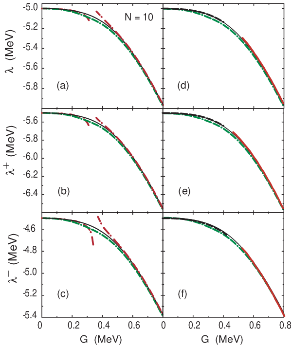
The quantities that are directly defined by the differences of ground-state energies are the chemical potentials $\lambda^{\pm}$ and $\lambda$ , namely

\lambda^{+}=\frac{1}{2}\left[E_{\rm g.s.}(N+2)-E_{\rm g.s.}(N)\right]~,\hskip 14.22636pt\lambda^{-}=\frac{1}{2}\left[E_{\rm g.s.}(N)-E_{\rm g.s.}(N-2)\right]~,\hskip 14.22636pt\lambda=\frac{1}{2}(\lambda^{+}+\lambda^{-})~.

(65)

The exact values of the chemical potentials $\lambda$ and $\lambda^{\pm}$ are shown in Fig. 3 in comparison with the predictions within quasiparticle presentations for $N=$ 10. It is seen from this figure that the SCRPA and SCQRPA [Fig. 3 (d) - 3 (f)] offer the best fit to the exact results except that the SCRPA poorly converges at $G>$ 0.4 MeV, while SCQRPA stops at $G=G_{\rm cr}^{\rm BCS1}$ . The RPA and QRPA also describe very well the exact results, except the values in the critical region, where the RPA and QRPA diverge. The LNSCQRPA predictions for the chemical potentials show smooth functions at all $G$ , which fit well the exact results, including the region around $G_{\rm cr}$ , where they slightly underestimates the exact ones.

III.3 Energies of excited state

As has been discussed in Refs. QRPA1; SCQRPA2, the first solution $\omega_{1}$ of the QRPA or SCQRPA equations is the energy of spurious mode, which is well separated from the physical solutions $\omega_{\nu}$ with $\nu\geq$ 2. The first excited state energy is therefore given by $\omega_{2}$ . Figure 4 shows the exact eigenvalues for the excited states. As has also been demonstrated in Ref. exact3, this figure shows that the coupling in the small-G region causes only small perturbations in the single-particle levels. With increasing $G$ the system goes to the crossover regime, where level splitting and crossing are seen, releasing the levels’ degeneracy. In the strong coupling regime the levels coalesce into narrow well-separated bands. The approaches based on the QRPA with PNP within the LN method also splits the levels but the nature of the splitting comes from the two components within the QRPA operator (40), which correspond to the addition and removal modes, respectively, in the RPA limit. When the pairing gap $\Delta$ is finite, it is not possible to consider the QRPA excitations as purely addition or removal modes, but only as those with some components having the dominating property inherent to one of these modes. The QRPA eigenvalues also have two branches with positive $\omega_{\nu}$ and negative $-\omega_{\nu}$ energies. However, unlike the $pp$ RPA, where the negative eigenvalues in the equations for addition modes are also physical as they are the energies of the removal modes taken with the minus sign and vice versa, within the QRPA only the positive energies $\omega_{\nu}$ are physical, and they are compared with the exact ones, $E_{\nu}^{ex}\equiv{\cal E}_{\nu}(N)-{\cal E}_{0}(N)$ , in the present paper.

As an example to illustrate this level-splitting pattern, we show in Fig. 5 the exact energy $E_{1}^{\rm ex}\equiv{\cal E}_{1}(N)-{\cal E}_{0}(N)$ of the lowest excited state ( $\nu=$ 1) with respect to the exact ground state ( $\nu=$ 0) in the system with $N=$ 10 particles in comparison with the predictions within the QRPA, LNQRPA, SCQRPA, and LNSCQRPA ³³ 3 For the two-level case $E_{1}^{\rm ex}$ corresponds to the solid line in the upper panel of Figs. 1, 3 – 5 in Ref. SCQRPA2 or Figs. 1 – 3 in Ref. Samba for $N=$ 4, 8, and 12).. As the exact energy $E_{1}^{\rm ex}$ represents the energy of the lowest pair-vibration state, it is compared with the energies $\omega_{1}$ of the lowest excited state obtained within QRPA, LNQRPA, SCQRPA and LNSCQRPA, which are built on the pairing condensate (quasiparticle vacuum). The splitting is clearly seen from Fig. 5 within the LN method, namely the LNQRPA and LNSCQRPA. One can see that, within the LN(SC)QRPA, each single level at $G=$ 0 splits into two components in the small-G region, e.g. the pair $\omega_{2}^{\rm LNQRPA}$ and $\omega_{3}^{\rm LNQRPA}$ or $\omega_{2}^{\rm LNSCQRPA}$ and $\omega_{3}^{\rm LNSCQRPA}$ . To look inside the source of the splitting, we rewrite the QRPA operator (40) into the components with dominating contributions of addition- and removal-mode patterns as follows:

Q_{\nu}^{\dagger}=(Q_{\nu}^{\dagger})^{(\rm A)}+(Q_{\nu}^{\dagger})^{(\rm R)}~,\hskip 14.22636pt

(Q_{\nu}^{\dagger})^{(\rm A)}=\sum_{p}X_{p}^{\nu}\mathcal{A}_{p}^{\dagger}-\sum_{h}Y_{h}^{\nu}\mathcal{A}_{h}~,\hskip 14.22636pt(Q_{\nu}^{\dagger})^{(\rm R)}=\sum_{h}X_{h}^{\nu}\mathcal{A}_{h}^{\dagger}-\sum_{p}Y_{p}^{\nu}\mathcal{A}_{p}~,

(66)

where the indices $j$ run over all the levels, from which those located below (above) the chemical potential are formally labelled with $h$ ( $p$ ) indices. It is not difficult to see that, in the RPA limit (or zero-pairing limit), $(Q_{\nu}^{\dagger})^{(\rm A)}$ is transformed into operator $A_{\nu}^{\dagger}$ that generates the addition modes, while $(Q_{\nu}^{\dagger})^{(\rm R)}$ becomes $R_{\nu}^{\dagger}$ that generates the removal modes (in the standard notations for addition and removal operators from Refs. SCRPA1; SCRPA2; SCRPA3). Using this formal expression (66), we derived the QRPA equations for the excitations generated by operators $(Q_{\nu}^{\dagger})^{(\rm A)}$ and $(Q_{\nu}^{\dagger})^{(\rm R)}$ , separately. The energies of the corresponding first excited states from the resulting sets of equations were calculated by using the LN method. We call this scheme as LNQRPA1. The set of equations for the modes generated by operator $(Q_{\nu}^{\dagger})^{(\rm A)}$ gives a negative $\omega_{2}^{\rm LNQRPA1}$ and positive $\omega_{3}^{\rm LNQRPA1}$ , which means that they correspond to the energies of the removal and addition modes, respectively. The absolute values of these energies are shown in Fig. 6 along with $\omega_{2,3}^{\rm LNQRPA}$ . It is seen from this figure that in the weak-coupling region the higher-lying levels $\omega_{3}^{\rm LNQRPA}$ and $\omega_{3}^{\rm LNQRPA1}$ nearly coincide, while the lower-lying one, $\omega_{2}^{\rm LNQRPA}$ , is almost the same as $|\omega_{2}^{\rm LNQRPA1}|$ . From here, we can identify $\omega_{3}^{\rm LNQRPA}$ and $\omega_{2}^{\rm LNQRPA}$ as the levels where the addition and removal modes dominate, respectively. As the interaction $G$ increases, the occupation probabilities of the levels below and above the Fermi level become comparable so it becomes more and more difficult to separate the patterns belonging to addition and removal modes in the QRPA excitations.

From this analysis and Fig. 5, it becomes clear that, in the weak coupling region, the level $\omega_{3}^{\rm LNQRPA}$ , which is generated mainly by the addition mode, fits well the exact result, while the agreement between the exact energy and $\omega_{2}^{\rm QRPA}$ as well as $\omega_{2}^{\rm SCQRPA}$ is good only in the strong coupling region. At large values of $G$ , predictions by all approximations and the exact solution coalesce into one band, whose width vanishes in the limit $G\rightarrow\infty$ .

The energies of the ground state and the first excited state obtained for $N=$ 4, 6, 8 are depicted in Fig. 7. The figure shows that increasing $N$ worsens the agreement of the results obtained within the LNQRPA and LNSCQPPA with the exact ones for both the ground state and the first excited state, while the QRPA and SCQRPA results become closer to the exact ones at $G\gg G_{\rm cr}$ . At small $N$ ( $N=$ 4), the solution $\omega_{3}^{\rm LNQRPA}$ seems to fit best the exact result for all values of $G$ .

The pair-vibration excitation energy $E_{1}^{\rm ex}$ is usually larger than the energy of the lowest state with one broken pair. The latter is described within the $pp$ RPA as the energy of the lowest addition mode in the laboratory reference frame fixed to the ground state of $N$ -particle system SCRPA1; SCRPA2; SCRPA3. It is worthwhile to compare the predictions for the excited-state energies obtained within the quasiparticle approaches developed in the present paper with $pp$ RPA and SCRPA predictions by transforming the latter into the intrinsic reference frame of the system with $N+2$ particles. This is done as follows. From the (SC)RPA energy of the ground-state level ${\omega}_{0}^{\rm(SC)RPA}={\cal E}_{0}^{\rm(SC)RPA}(N+2)-{\cal E}_{0}^{\rm(SC)RPA}(N)$ , and that of the first excited state ${\omega}_{1}^{\rm(SC)RPA}={\cal E}_{1}^{\rm(SC)RPA}(N+2)-{\cal E}_{0}^{\rm(SC)RPA}(N)$ ⁴⁴ 4 The energies ${\omega}_{0}^{\rm(SC)RPA}$ and ${\omega}_{1}^{\rm(SC)RPA}$ correspond to energies $E_{1}$ and $E_{2}$ shown in Figs. 3 and 4 in Ref. SCRPA1, respectively. it follows that

\Delta\omega^{\rm(SC)RPA}\equiv{\omega}_{1}^{\rm(SC)RPA}-{\omega}_{0}^{\rm(SC)RPA}={\cal E}_{1}^{\rm(SC)RPA}(N+2)-{\cal E}_{0}^{\rm(SC)RPA}(N+2)~,

(67)

This energy $\Delta\omega^{\rm(SC)RPA}$ is shown in Fig. 8 as a function of $G$ along with the corresponding LNQRPA, LNSCQRPA, and exact energies for several values of $N$ . This figure clearly shows that the LNQRPA and LNSCQRPA are superior to the $pp$ RPA and SCRPA as they offer an overall prediction closer to the exact result for all $G$ and $N$ . They neither collapse at a $G_{\rm cr}$ as in the case with the $pp$ RPA nor have a poor convergence as the SCRPA does at $G\gg G_{\rm cr}$ .

IV Conclusions

This work proposes a self-consistent version of the QRPA in combination with particle-number projection within the Lipkin-Nogami method as an approach that works at any values of the pairing-interaction parameter $G$ without suffering a phase-transition-like collapse (or poor convergence) due to the violation of Pauli principle as well as of the integral of motion such as the particle number. The self-consistency is maintained within a set of coupled equations for the pairing gap, QRPA amplitudes, and energies by means of the screening factors, which are the expectation values of the products of quasiparticle-pair operators, and the ground-state correlation factor, which is a function of the QRPA backward-going amplitudes.

The proposed approach is tested in a multi-level exactly solvable model, namely the Richardson model for pairing. The energies of the ground and first-excited states are calculated within several approximations such as the BCS, RBCS, BCS1, LN, RLN, LN1, QRPA, SCQRPA, LNQRPA and LNSCQRPA. The obtained results for the ground-state energy show that the use of the LN method that includes the SCQRPA correlations not only allows us to avoid the collapse of the BCS as well as the QRPA but also fits well the exact result. For the energy of the first excited state, the LNQRPA and LNSCQRPA results offer the best fits to the exact solutions in the weak coupling region with large particle numbers, while the QRPA and SCQRPA reproduce well the exact one in the strong coupling region. In the limit of very large $G$ all the approximations predict nearly the same value as that of the exact one. As the number of particles decreases, it becomes sufficiently well to use the predictions given by the LNQRPA and LNSCQRPA for energies of both the ground state and first-excited state to fit the exact results.

We believe that the approach proposed in this work can be useful in the applications to light and unstable nuclei, where the validity of the QBA and that of the conventional BCS are in question. Such applications are the goal for forthcoming studies.

Acknowledgements.

The authors are grateful to Michelangelo Sambataro (Catania) for his assistance in the exact solutions of the Richardson model. The numerical calculations were carried out using the FORTRAN IMSL Library by Visual Numerics on the RIKEN Super Combined Cluster (RSCC) system. NQH is a RIKEN Asian Program Associate.

Appendix A Accuracy of approximation (33)

Table 3: BCS1 and LN1 pairing gaps (in MeV) at various values of G (in MeV) (see text).

	BCS1			LN1
G	$\Delta$	$\overline{\Delta}$	$\frac{\delta\Delta}{\Delta}~(\%)$	$\widetilde{\Delta}$	$\overline{\widetilde{\Delta}}$	$\frac{\delta\tilde{\Delta}}{\tilde{\Delta}}~(\%)$
0.01				0.0015	0.0015	0.0000
0.10				0.0606	0.0607	0.1647
0.20				0.2279	0.2289	0.4369
0.30				0.5278	0.5321	0.8081
0.40				0.9579	0.9660	0.8385
0.47	0.8224	0.8357	1.5915	1.3139	1.3233	0.7103
0.50	1.0694	1.0829	1.2467	1.4742	1.4839	0.6537
0.60	1.7219	1.7351	0.7608	2.0261	2.0360	0.4862
0.70	2.3314	2.3436	0.5206	2.5896	2.5993	0.3617
0.80	2.9279	2.9391	0.3811	3.1541	3.1633	0.2908
0.90	3.5132	3.5235	0.2923	3.7148	3.7234	0.2310
1.00	4.0882	4.0977	0.2318	4.2701	4.2783	0.1917
1.10	4.6539	4.6629	0.1930	4.8197	4.8277	0.1657
1.20	5.2118	5.2203	0.1628	5.3641	5.3718	0.1433
1.30	5.7628	5.7710	0.1421	5.9037	5.9113	0.1286
1.40	6.3079	6.3160	0.1282	6.4390	6.4466	0.1179

Table 4: The ratio

(\delta{\cal N}_{j})^{2}/\langle{\cal D}_{j}\rangle

from Eqs. (31) and (32) corresponding to the 5 lowest levels

j=

1, …, 5, and the energies

\omega_{3}

(in MeV) of the first excited state described in the text for

N=

10 at different values of

G

(in MeV) within the LNSCQRPA. The energy

\omega_{3}(a)

is obtained including the last term at the rhs of Eq. (31), while

\omega_{3}(b)

is calculated using the approximation (33).

G	$j=1$	$j=2$	$j=3$	$~~j=4$	$~~j=5$	$\omega_{3}(a)$	$\omega_{3}(b)$
0.01	0.0000	0.0000	0.0000	0.0000	0.0000	2.0001	2.0001
0.2	0.0009	0.0012	0.0017	0.0027	0.0046	2.0697	2.0711
0.4	0.0023	0.0030	0.0040	0.0055	0.0082	2.6701	2.6742
0.6	0.0019	0.0023	0.0027	0.0032	0.0054	4.2040	4.2067
0.8	0.0013	0.0015	0.0016	0.0021	0.0033	6.1514	6.1531
1.0	0.0009	0.0010	0.0011	0.0015	0.0022	8.1798	8.1812
1.2	0.0006	0.0007	0.0009	0.0012	0.0017	10.211	10.212
1.4	0.0005	0.0006	0.0008	0.0011	0.0014	12.229	12.230

Let us analyze the accuracy of the assumption (33) used in the numerical solutions of the BCS1, LN1, and SCQRPA equations in the present paper.

Shown in the 2nd and 5th columns of Table 3 are the values of the pairing gaps $\Delta$ and $\widetilde{\Delta}$ obtained under the approximation (33) within the BCS1 and LN1 method, respectively. They are compared with the average gaps $\overline{\Delta}$ (3rd column) and $\overline{\widetilde{\Delta}}$ (6th column), which are the values obtained by averaging the level-dependent BCS1 gap $\Delta_{j}$ and LN1 gap $\widetilde{\Delta}_{j}$ over all the levels, namely $\overline{\Delta}=\sum_{j}\Delta_{j}/N$ and $\overline{\widetilde{\Delta}}=\sum_{j}\widetilde{\Delta}_{j}/N$ . The second term at the rhs of Eq. (31), which contains $\delta{\cal N}_{j}^{2}$ as evaluated by the approximation (32), is taken into account in calculating $\Delta_{j}$ and $\widetilde{\Delta}_{j}$ within the perturbation theory, i.e. with $n_{j}$ being evaluated within SCQRPA and LNSCQRPA (where this term is neglected). Except for the two values at $G=G_{\rm cr}^{\rm BCS1}=$ 0.47 MeV and $G=$ 0.5 MeV within the BCS1, we see that the values of the relative errors $\delta\Delta/\Delta\equiv(\overline{\Delta}-\Delta)/\Delta$ and $\delta\widetilde{\Delta}/\widetilde{\Delta}\equiv(\overline{\widetilde{\Delta}}-\widetilde{\Delta})/\widetilde{\Delta}$ are all smaller than 1 $\%$ , and decrease with increasing $G$ .

Shown in Table 4 are the values of the ratio $(\delta{\cal N}_{j})^{2}/\langle{\cal D}_{j}\rangle$ from Eqs. (31) and (32) corresponding to the five lowest levels for $N=$ 10 at various $G$ obtained within the LNSCQRPA. The largest value of this ratio is observed at the level with $j=$ 5, the closest one to the Fermi level, at $G=$ 0.4 MeV (close to $G_{\rm cr}^{\rm BCS1}$ ). But it amounts to only 0.0082, which is a clear evidence that this ratio is indeed negligible. The last two columns of this table display the energies $\omega_{3}(a)$ , obtained within the LNSCQRPA including the last term at the rhs of Eq. (31), and $\omega_{3}(b)$ , which the LNSCQRPA predicts within the approximation (33). Although a systematic $\omega_{3}(a)>\omega_{3}(b)$ is observed, the largest difference, also seen at $G=$ 0.4 MeV, does not exceed 0.15 $\%$ . These results guarantee the high accuracy of the approximation (33).

References

(1) K. Hara, Prog. Theor. Phys. 32, 88 (1964); K. Ikeda, T. Udagawa, and H. Yamamura, ibid. 33, 22 (1965); P. Schuck and S. Ethofer, Nucl. Phys. A 212, 269 (1973).
(2) D. J. Rowe, Phys. Rev. 175, 1283 (1968).
(3) F. Catara, N. D. Dang, and M. Sambataro, Nucl. Phys. A 579, 1 (1994)
(4) J. Dukelsky and P. Schuck, Phys. Lett. B 464, 164 (1999).
(5) J. G. Hirsch, A. Mariano, J. Dukelsky, and P. Schuck, Ann. Phys. (NY) 296, 187 (2002).
(6) N. D. Dang, Phys. Rev. C 71, 024302 (2005).
(7) N.D. Dang and K. Tanabe, Phys. Rev. C 74, 034326 (2006).
(8) J. Dukelsky and P. Schuck, Phys. Lett. B 387, 233 (1996)
(9) A. Rabhi, R. Bennaceur, G. Chanfray, and P. Schuck, Phys. Rev. C 66, 064315(2002).
(10) H. J. Lipkin, Ann. Phys. (NY) 9 272 (1960); Y. Nogami and I. J. Zucker, Nucl. Phys. 60 203 (1964); Y. Nogami, Phys. Lett. 15 4 (1965); J. F. Goodfellow and Y. Nogami, Can. J. Phys. 44 1321 (1966).
(11) H.C. Pradhan, Y. Nogami, and J. Law, Nucl. Phys. A 201, 357 (1973)
(12) R. W. Richardson, Phys. Lett. 3, 277 (1963); Ibid. 14, 325 (1965).
(13) J. Högaasen-Feldman, Nucl. Phys. 28, 258 (1961).
(14) N. D. Dang, Z. Phys. A 335, 253 (1990).
(15) N. Dinh Dang and A. Arima, Phys. Rev. C 67, 014304 (2003).
(16) J. Dukelsky and P. Schuck, Nucl. Phys. A 512, 466 (1990).
(17) M. Sambataro and N. Dinh Dang, Phys. Rev. C 59, 1422 (1999).
(18) A. Valor, J.L. Egido, and L.M. Robledo, Nucl. Phys. A 665, 46 (2000); T.R. Rodriguez, J.L. Egido, and L.M. Robledo, Phys. Rev. C 72, 064303 (2005).
(19) P. Magierski, S. Cwiok, J. Dobaczewski, and W. Nazarewicz, Phys. Rev. C 48, 1686 (1993).
(20) N. D. Dang, Eur. Phys. J. A 16, 181 (2003).
(21) A. Volya, B. A. Brown, V. Zelevinsky, Phys. Lett. B 509, 37 (2001)
(22) E. A. Yuzbashyan, A. A. Baytin, B. L. Altshuler, Phys. Rev. B 68, 214509 (2003).