跳到论文正文
W Papers独立论文阅读器 arXiv:0710.0900 论文正文 计算阅读时间 · 0%
引用这篇论文根据当前论文元数据生成,正式投稿前建议核对。


License: Assumed arXiv.org perpetual non-exclusive license
arXiv:0710.0900v1 [cs.IT] 04 Oct 2007

A New Achievability Scheme for the Relay ChannelThanks: This work was supported by NSF Grants CCR 0303-1131111311, CCF 0404-4761347613 and CCF 0505-1484614846, and was presented in part at IEEE Information Theory Workshop, Lake Tahoe, CA, September 2007.

Wei Kang    Sennur Ulukus Affiliation: Department of Electrical and Computer Engineering Affiliation: University of Maryland, College Park, MD 20742 Email: wkang@umd.edu    ulukus@umd.edu
Abstract

In this paper, we propose a new coding scheme for the general relay channel. This coding scheme is in the form of a block Markov code. The transmitter uses a superposition Markov code. The relay compresses the received signal and maps the compressed version of the received signal into a codeword conditioned on the codeword of the previous block. The receiver performs joint decoding after it has received all of the BB blocks. We show that this coding scheme can be viewed as a generalization of the well-known Compress-And-Forward (CAF) scheme proposed by Cover and El Gamal. Our coding scheme provides options for preserving the correlation between the channel inputs of the transmitter and the relay, which is not possible in the CAF scheme. Thus, our proposed scheme may potentially yield a larger achievable rate than the CAF scheme.

1 Introduction

As the simplest model for cooperative communications, relay channel has attracted plenty of attention since 1971, when it was first introduced by van der Meulen [1]. In 1979, Cover and El Gamal proposed two major coding schemes for the relay channel [2]. These two schemes are widely known as Decode-And-Forward (DAF) and Compress-And-Forward (CAF) today; see [3] for a recent review. These two coding schemes represent two different types of cooperation. In DAF, the cooperation is relatively obvious, where the relay decodes the message from the transmitter, and the transmitter and the relay cooperatively transmit the constructed common information to the receiver in the next block. In CAF, the cooperation spirit is less easy to recognize, as the message is sent by the transmitter only once. However, the relay cooperates with the transmitter by compressing and sending its signal to the receiver. The rate gains in these achievable schemes are due to the fact that, through the channel from the transmitter to the relay, correlation is created between the transmitter and the relay, and this correlation is utilized to improve the rates.

In the DAF scheme, correlation is created and then utilized in a block Markov coding structure. More specifically, a full correlation is created by decoding the message fully at the relay, which enables the transmitter and the relay to create any kind of joint distribution for the channel inputs in the next block. The shortcoming of the DAF scheme is that by forcing the relay to decode the message in its entirety, it limits the overall achievable rate by the rate from the transmitter to the relay. In contrast, by not forcing a full decoding at the relay, the CAF scheme does not limit the overall rate by the rate from the transmitter to the relay, and may yield higher overall rates. The shortcoming of the CAF scheme, on the other hand, is that the correlation offered by the block coding structure is not utilized effectively, since in each block the channel inputs XX and X1X_{1} from the transmitter and the relay are independent, as the transmitter sends the message only once.

However, the essence of good coding schemes in multi-user systems with correlated sources (e.g., [4, 5]) is to preserve the correlation of the sources in the channel inputs. Motivated by this basic observation, in this paper, we propose a new coding scheme for the relay channel, that is based on the idea of preserving the correlation in the channel inputs from the transmitter and the relay. We will show that our new coding scheme may be viewed as a more general version of the CAF scheme, and therefore, our new coding scheme may potentially yield larger rates than the CAF scheme. Our proposed scheme can be further combined with the DAF scheme to yield rates that are potentially larger than those offered by both DAF and CAF schemes, similar in spirit to [2, Theorem 7].

Our new achievability scheme for the relay channel may be viewed as a variation of the coding scheme of Ahlswede and Han [5] for the multiple access channel with a correlated helper. In our work, we view the relay as the helper because the receiver does not need to decode the information sent by the relay. Also, we note that the relay is a correlated helper as the communication channel from the transmitter to the relay provides relay for free a correlated version of the signal sent by the transmitter. The key aspects of the Ahlswede-Han [5] scheme are: to preserve the correlation between the channel inputs of the transmitter and the helper (relay), and for the receiver to decode a “virtual” source, a compressed version of the helper, but not the entire signal of the helper.

Our new coding scheme is in the form of block Markov coding. The transmitter uses a superposition Markov code, similar to the one used in the DAF scheme [2], except in the random codebook generation stage, a method similar to the one in [4] is used in order to preserve the correlation between the blocks. Thus, in each block, the fresh information message is mapped into a codeword conditioned on the codeword of the previous block. Therefore, the overall codebook at the transmitter has a tree structure, where the codewords in block ll emanate from the codewords in block l−1l-1. The depth of the tree is B−1B-1. A similar strategy is applied at the relay side where the compressed version of the received signal is mapped into a two-block-long codeword conditioned on the codeword of the previous block. Therefore, the overall codebook at the relay has a tree structure as well. As a result of this coding strategy, we successfully preserve the correlation between the channel inputs of the transmitter and the relay. However, unlike the DAF scheme where a full correlation is acquired through decoding at the relay, our scheme provides only a partially correlated helper at the relay by not trying to decode the transmitter’s signal fully. From [4, 5], we note that the channel inputs are correlated through the virtual sources in our case, and therefore, the channel inputs between the consecutive blocks are correlated. This correlation between the blocks will surely hurt the achievable rate. The correlation between the blocks is the price we pay for preserving the correlation between the channel inputs of the transmitter and the relay within any given block.

At the decoding stage, we perform joint decoding for the entire BB blocks after all of the BB blocks have been received, which is different compared with the DAF and CAF schemes. The reason for performing joint decoding at the receiver is that due to the correlation between the blocks, decoding at any time before the end of all the BB blocks would decrease the achievable rate. We note that joint decoding increases the decoding complexity and the delay as compared to DAF and CAF, though neither of these is a major concern in an information theoretic context. The only problem with the joint decoding strategy is that it makes the analysis difficult as it requires the evaluation of some mutual information expressions involving the joint probability distributions of up to BB blocks of codes, where BB is very large.

The analysis of the error events provides us three conditions containing mutual information expressions involving infinite letters of the underlying random process. Evaluation of these mutual information expressions is very difficult, if not impossible. To obtain a computable result, we lower bound these mutual informations by noting some Markov structure in the underlying random process. This operation gives us three conditions to be satisfied by the achievable rates. These conditions involve eleven variables, the two channel inputs from the transmitter and the relay, the two channel outputs at the relay and the receiver and the compressed version of the channel output at the relay, in two consecutive blocks, and the channel input from the transmitter in the previous block.

We finish our analysis by revisiting the CAF scheme. We develop an equivalent representation for the achievable rates given in [2] for the CAF scheme. We then show that this equivalent representation for the achievable rates for the CAF scheme is a special case of the achievable rates in our new coding scheme, which is obtained by a special selection of the eleven variables mentioned above. We therefore conclude that our proposed coding scheme yields potentially larger rates than the CAF scheme. More importantly, our new coding scheme creates more possibilities, and therefore a spectrum of new achievable schemes for the relay channel through the selection of the underlying probability distribution, and yields the well-known CAF scheme as a special case, corresponding to a particular selection of the underlying probability distribution.

2 The Relay Channel

Consider a relay channel with finite input alphabets 𝒳\mathcal{X}, 𝒳1\mathcal{X}_{1} and finite output alphabets 𝒴\mathcal{Y}, 𝒴1\mathcal{Y}_{1}, characterized by the transition probability p(y,y1|x,x1)p(y,y_{1}|x,x_{1}). An nn-length block code for the relay channel p(y,y1|x,x1)p(y,y_{1}|x,x_{1}) consists of encoders f,fif,f_{i}, i=1,…,ni=1,\dots,n and a decoder gg

f\displaystyle f :ℳ⟶𝒳n\displaystyle:\mathcal{M}\longrightarrow\mathcal{X}^{n}
fi\displaystyle f_{i} :𝒴1i−1⟶𝒳1,i=1,…,n\displaystyle:\mathcal{Y}_{1}^{i-1}\longrightarrow\mathcal{X}_{1},\qquad i=1,\dots,n
g\displaystyle g :𝒴n⟶ℳ\displaystyle:\mathcal{Y}^{n}\longrightarrow\mathcal{M}

where the encoder at the transmitter sends xn=f⁡(m)x^{n}=f(m) into the channel, where m∈ℳ≜{1,2,…,M}m\in\mathcal{M}\triangleq\{1,2,\dots,M\}; the encoder at the relay at the iith channel instance sends x1​i=fi​(y1i−1)x_{1i}=f_{i}(y_{1}^{i-1}) into the channel; the decoder outputs m^=g⁡(yn)\hat{m}=g(y^{n}). The average probability of error is defined as

Pe=1M​∑m∈ℳP​r​(m^≠m|m​is transmitted)P_{e}=\frac{1}{M}\sum_{m\in\mathcal{M}}Pr(\hat{m}\neq m|m~\text{is transmitted}) (1)

A rate RR is achievable for the relay channel p(y,y1|x,x1)p(y,y_{1}|x,x_{1}) if for every 0<ϵ<10<\epsilon<1, η>0\eta>0, and every sufficiently large nn, there exists an nn-length block code (f,fi,g)(f,f_{i},g) with Pe≤ϵP_{e}\leq\epsilon and 1n​ln⁡M≥R−η\frac{1}{n}\ln M\geq R-\eta.

3 A New Achievability Scheme for the Relay Channel

We adopt a block Markov coding scheme, similar to the DAF and CAF schemes. We have overall BB blocks. In each block, we transmit codewords of length nn. We denote the variables in the llth block with a subscript of [l][l]. We denote nn-letter codewords transmitted in each block with a superscript of nn. Following the standard relay channel literature, we denote the (random) signals transmitted by the transmitter and the relay by XX and X1X_{1}, the signals received at the receiver and the relay by YY and Y1Y_{1}, and the compressed version of Y1Y_{1} at the relay by Y^1\hat{Y}_{1}. The realizations of these random signals will be denoted by lower-case letters. For example, the nn-letter signals transmitted by the transmitter and the relay in the llth block will be represented by x[l]nx_{[l]}^{n} and x1​[l]nx_{1[l]}^{n}.

Consider the following discrete time stationary Markov process G[l]≜(X,Y^1,X1,y,Y1)[l]G_{[l]}\triangleq(X,\hat{Y}_{1},X_{1},y,Y_{1})_{[l]} for l=0,1,…,Bl=0,1,\dots,B, with the transition probability distribution

p⁡((x,y^1,x1,y,y1)[l]|(x,y^1,x1,y,y1)[l−1])\displaystyle p\left((x,\hat{y}_{1},x_{1},y,y_{1})_{[l]}|(x,\hat{y}_{1},x_{1},y,y_{1})_{[l-1]}\right)
=p⁡(x[l]|x[l−1])​p\displaystyle=p(x_{[l]}|x_{[l-1]})p (y1​[l],y[l]|x[l],x1​[l])p(x1​[l]|y^1​[l−1])p(y^1​[l]|y1​[l],x1​[l])\displaystyle(y_{1[l]},y_{[l]}|x_{[l]},x_{1[l]})p(x_{1[l]}|\hat{y}_{1[l-1]})p(\hat{y}_{1[l]}|y_{1[l]},x_{1[l]}) (2)

The codebook generation and the encoding scheme for the llth block, l=1,…,B−1l=1,\dots,B-1, are as follows.

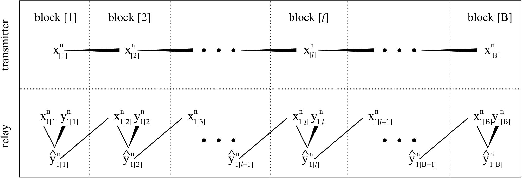
Random codebook generation: Let (x[l−1]n​(m[l−1]),x1​[l−1]n,y1​[l−1]n,y[l−1]n)(x_{[l-1]}^{n}(m_{[l-1]}),x_{1[l-1]}^{n},y_{1[l-1]}^{n},y_{[l-1]}^{n}) denote the transmitted and the received signals in the (l−1)(l-1)st block, where m[l−1]m_{[l-1]} is the message sent by the transmitter in the (l−1)(l-1)st block. An illustration of the codebook structure is shown in Figure 1.

  1. 1.

    For each x[l−1]n​(m[l−1])x_{[l-1]}^{n}(m_{[l-1]}) sequence, generate MM sequences, where x[l]n​(m[l])x^{n}_{[l]}(m_{[l]}), the m[l]m_{[l]}th sequence, is generated independently according to ∏i=1np⁡(xi⁡[l]|xi⁡[l−1])\prod_{i=1}^{n}p(x_{i[l]}|x_{i[l-1]}). Here, every codeword in the (l−1)(l-1)st block expands into a codebook in the llth block. This expansion is indicated by a directed cone from x[l−1]nx_{[l-1]}^{n} to x[l]nx_{[l]}^{n} in Figure 1.

  2. 2.

    For each x1​[l−1]nx_{1[l-1]}^{n} sequence, generate LL Y^1​[l−1]n\hat{Y}_{1[l-1]}^{n} sequences independently uniformly distributed in the conditional strong typical set11 1 Strong typical set and conditional strong typical set are defined in [6, Definition 1.2.8, 1.2.9]. For the sake of simplicity, we omit the subscript which is used to indicate the underlying distribution in [6]. 𝒯δ​(x1​[l−1]n)\mathcal{T}_{\delta}(x_{1[l-1]}^{n}) with respect to the distribution p⁡(y^1​[l−1]|x1​[l−1])p(\hat{y}_{1[l-1]}|x_{1[l-1]}). If 1n​ln⁡L>I⁡(Y1​[l−1];Y^1​[l−1]|X1​[l−1])\frac{1}{n}\ln L>I(Y_{1[l-1]};\hat{Y}_{1[l-1]}|X_{1[l-1]}), for any given y1​[l−1]ny_{1[l-1]}^{n} sequence, there exists one y^1​[l−1]n\hat{y}_{1[l-1]}^{n} sequence with high probability when nn is sufficiently large such that (y1​[l−1]n,y^1​[l−1]n,x1​[l−1]n)(y_{1[l-1]}^{n},\hat{y}_{1[l-1]}^{n},x_{1[l-1]}^{n}) are jointly typical according to the probability distribution p⁡(y1​[l−1],y^1​[l−1],x1​[l−1])p(y_{1[l-1]},\hat{y}_{1[l-1]},x_{1[l-1]}). Denote this y^1​[l−1]n\hat{y}_{1[l-1]}^{n} as y^1​[l−1]n​(y1​[l−1]n,x1​[l−1]n)\hat{y}_{1[l-1]}^{n}(y_{1[l-1]}^{n},x_{1[l-1]}^{n}). Here, the quantization from y1​[l−1]ny_{1[l-1]}^{n} to y^1​[l−1]n\hat{y}_{1[l-1]}^{n}, parameterized by x1​[l−1]nx_{1[l-1]}^{n}, is indicated in Figure 1 by a directed cone from y1​[l−1]ny_{1[l-1]}^{n} to y^1​[l−1]n\hat{y}_{1[l-1]}^{n}, with a straight line from x1​[l−1]nx_{1[l-1]}^{n} for the parameterization.

  3. 3.

    For each y^1​[l−1]n\hat{y}_{1[l-1]}^{n}, generate one x1​[l]nx_{1[l]}^{n} sequence according to ∏i=1np⁡(x1​i​[l]|y^1​i​[l−1])\prod_{i=1}^{n}p(x_{1i[l]}|\hat{y}_{1i[l-1]}). This one-to-one mapping is indicated by a straight line between y^1​[l−1]n\hat{y}_{1[l-1]}^{n} and x1​[l]nx_{1[l]}^{n} in Figure 1.

Refer to caption
Figure 1: Codebook structure.

Encoding: Let m[l]m_{[l]} be the message to be sent in this block. If (x[l−1]n​(m[l−1]),x1​[l−1]n)(x_{[l-1]}^{n}(m_{[l-1]}),x_{1[l-1]}^{n}) are sent and y1​[l−1]ny_{1[l-1]}^{n} is received in the previous block, we choose (x[l]n​(m[l]),y^1​[l−1]n​(y1​[l−1]n,x1​[l−1]n),x1​[l]n)(x^{n}_{[l]}(m_{[l]}),\hat{y}_{1[l-1]}^{n}(y_{1[l-1]}^{n},x_{1[l-1]}^{n}),x_{1[l]}^{n}) according to the code generation method described above and transmit (x[l]n​(m[l]),x1​[l]n)(x^{n}_{[l]}(m_{[l]}),x_{1[l]}^{n}). In the first block, we assume a virtual 00th block, where (x[0]n,x1​[0]n,y^1​[0]n)(x^{n}_{[0]},x^{n}_{1[0]},\hat{y}^{n}_{1[0]}), as well as x1​[1]nx^{n}_{1[1]}, are known by the transmitter, the relay and the receiver. In the BBth block, the transmitter randomly generates one x[B]nx_{[B]}^{n} sequence according to ∏i=1np⁡(xi⁡[B]|xi⁡[B−1])\prod_{i=1}^{n}p(x_{i[B]}|x_{i[B-1]}) and sends it into the channel. The relay, after receiving y1​[B]ny_{1[B]}^{n}, randomly generates one y^1​[B]n\hat{y}_{1[B]}^{n} sequence according to ∏i=1np⁡(y^1​i​[B]|y1​i​[B],x1​i​[B])\prod_{i=1}^{n}p(\hat{y}_{1i[B]}|y_{1i[B]},x_{1i[B]}). We assume that the transmitter and the relay reliably transmit x[B]nx_{[B]}^{n} and y^1​[B]n\hat{y}_{1[B]}^{n} to the receiver using the next bb blocks, where bb is some finite positive integer. We note that B+bB+b blocks are used in our scheme, while only the first B−1B-1 blocks carry the message. Thus, the final achievable rate is B−1B+b​1n​ln⁡M\frac{B-1}{B+b}\frac{1}{n}\ln M which converges to 1n​ln⁡M\frac{1}{n}\ln M for sufficiently large BB since bb is finite.

Decoding: After receiving BB blocks of yny^{n} sequences, i.e., y[1]n,…,y[B]ny^{n}_{[1]},\dots,y^{n}_{[B]}, and assuming x1​[1]nx^{n}_{1[1]}, x[B]nx^{n}_{[B]} and y^1​[B]n\hat{y}_{1[B]}^{n} are known at the receiver, we seek x[1]n,…,x[B−1]nx^{n}_{[1]},\dots,x^{n}_{[B-1]}, y^1​[1]n,…,y^1​[B−1]n,x1​[2]n,…,x1​[B]n\hat{y}^{n}_{1[1]},\dots,\hat{y}^{n}_{1[B-1]},x^{n}_{1[2]},\dots,x^{n}_{1[B]}, such that

(x[1]n,…,x[B]n,y^1​[1]n,…,y^1​[B]n,x1​[1]n,…,x1​[B]n,y[1]n,…,y[B]n)∈𝒯δ\left(x^{n}_{[1]},\dots,x^{n}_{[B]},\hat{y}^{n}_{1[1]},\dots,\hat{y}^{n}_{1[B]},x^{n}_{1[1]},\dots,x^{n}_{1[B]},y^{n}_{[1]},\dots,y^{n}_{[B]}\right)\in\mathcal{T}_{\delta}

according to the stationary distribution of the Markov process G[l]G_{[l]} in (3).

The differences between our scheme and the CAF scheme are as follows. At the transmitter side, in our scheme, the fresh message m[l]m_{[l]} is mapped into the codeword x[l]nx_{[l]}^{n} conditioned on the codeword of the previous block x[l−1]nx_{[l-1]}^{n}, while in the CAF scheme, m[l]m_{[l]} is mapped into x[l]nx_{[l]}^{n}, which is generated independent of x[l−1]nx_{[l-1]}^{n}. At the relay side, in our scheme, the compressed received signal y^1​[l−1]n\hat{y}_{1[l-1]}^{n} is mapped into the codeword x1​[l]nx_{1[l]}^{n}, which is generated according to p⁡(x1​[l]|y^1​[l−1])p(x_{1[l]}|\hat{y}_{1[l-1]}), while in the CAF scheme, x1​[l]nx_{1[l]}^{n} is generated independent of y^1​[l−1]n\hat{y}_{1[l-1]}^{n}. The aim of our design is to preserve the correlation built in the (l−1)(l-1)st block in the channel inputs of the llth block. At the decoding stage, we perform joint decoding for the entire BB blocks after all of the BB blocks have been received, while in the CAF scheme, the decoding of the message of the (l−1)(l-1)st block is performed at the end of the llth block.

Probability of error: When nn is sufficiently large, the probability of error can be made arbitrarily small when the following conditions are satisfied.

  1. 1.

    For all jj such that 1≤j≤B−11\leq j\leq B-1,

    1n​(B−j)​ln⁡M+(B−j)\displaystyle\frac{1}{n}(B-j)\ln M+(B-j) I(Y^1​[l];Y1​[l]|X1​[l],X[l])\displaystyle I(\hat{Y}_{1[l]};Y_{1[l]}|X_{1[l]},X_{[l]})
    <I(X[j][B−1],Y^1​[j][B−1],X1​[j+1][B];Y[j][B],Y^1​[B],X[B]|X[j−1],X1​[j])\displaystyle<I(X_{[j]}^{[B-1]},\hat{Y}_{1[j]}^{[B-1]},X_{1[j+1]}^{[B]};Y_{[j]}^{[B]},\hat{Y}_{1[B]},X_{[B]}|X_{[j-1]},X_{1[j]}) (3)
  2. 2.

    For all j,kj,k such that 1≤j<k≤B−11\leq j<k\leq B-1,

    1n​(B−j)\displaystyle\frac{1}{n}(B-j) lnM+(B−k)I(Y^1​[l];Y1​[l]|X1​[l],X[l])\displaystyle\ln M+(B-k)I(\hat{Y}_{1[l]};Y_{1[l]}|X_{1[l]},X_{[l]})
    <I(X[j][B−1],Y^1​[k][B−1],X1​[k+1][B];Y[j][B],Y^1​[B],X1​[B],Y^1​[j][k−1],X1​[j+1][k]|X[j−1],X[j])\displaystyle<I(X_{[j]}^{[B-1]},\hat{Y}_{1[k]}^{[B-1]},X_{1[k+1]}^{[B]};Y_{[j]}^{[B]},\hat{Y}_{1[B]},X_{1[B]},\hat{Y}_{1[j]}^{[k-1]},X_{1[j+1]}^{[k]}|X_{[j-1]},X_{[j]}) (4)
  3. 3.

    For all j,kj,k such that 1≤k<j≤B−11\leq k<j\leq B-1,

    (j−k)​I​(Y^1​[l];Y1​[l]|X1​[l]CLOSE\displaystyle(j-k)I(\hat{Y}_{1[l]};Y_{1[l]}|X_{1[l]} ,X[l])+1n(B−j)lnM+(B−j)I(Y^1​[l];Y1​[l]|X1​[l],X[l])\displaystyle,X_{[l]})+\frac{1}{n}(B-j)\ln M+(B-j)I(\hat{Y}_{1[l]};Y_{1[l]}|X_{1[l]},X_{[l]})
    <I(X[j][B−1],Y^1​[k][B−1],X1​[k+1][B];Y[k][B],Y^1​[B],X[B]|X[k][j−1],X1​[k])\displaystyle<I(X_{[j]}^{[B-1]},\hat{Y}_{1[k]}^{[B-1]},X_{1[k+1]}^{[B]};Y_{[k]}^{[B]},\hat{Y}_{1[B]},X_{[B]}|X_{[k]}^{[j-1]},X_{1[k]}) (5)

where the subscript [l][l] on the left hand sides of (3), (4) and (5) indicates that the corresponding random variables belong to a generic sample g[l]g_{[l]} of the underlying random process in (3). The details of the calculation of the probability of error where these conditions are obtained can be found in Appendix A.1. The derivation uses standard techniques from information theory, such as counting error events, etc.

In the above conditions, we used the notation A[j][B]A_{[j]}^{[B]} as a shorthand to denote the sequence of random variables A[j],A[j+1],…,A[B]A_{[j]},A_{[j+1]},\dots,A_{[B]}. Consequently, we note that the mutual informations on the right hand sides of (3), (4) and (5) contain vectors of random variables whose lengths go up to BB, where BB is very large. In order to simplify the conditions in (3), (4) and (5), we lower bound the mutual information expressions on the right hand sides of (3), (4) and (5) by those that involve random variables that belong to up to three blocks. The detailed derivation of the following lower bounding operation can be found in Appendix A.2. The derivation uses standard techniques from information theory, such as the chain rule of mutual information, and exploiting the Markov structure of the involved random variables.

  1. 1.

    For all jj such that 1≤j≤B−11\leq j\leq B-1,

    (B−j)(1nlnM+I(Y^1​[l];Y1​[l]|X1​[l],X[l]))\displaystyle(B-j)\left(\frac{1}{n}\ln M+I(\hat{Y}_{1[l]};Y_{1[l]}|X_{1[l]},X_{[l]})\right)
    <(B−j)​I​(Y[l]CLOSE\displaystyle<(B-j)I(Y_{[l]} ;X[l],Y^1​[l],X1​[l]|X[l−2],X1​[l−1],Y[l−1])\displaystyle;X_{[l]},\hat{Y}_{1[l]},X_{1[l]}|X_{[l-2]},X_{1[l-1]},Y_{[l-1]}) (6)
  2. 2.

    For all j,kj,k such that 1≤j<k≤B−11\leq j<k\leq B-1,

    (k−j)​1n​ln⁡M+(B−k)\displaystyle(k-j)\frac{1}{n}\ln M+(B-k) (1nlnM+I(Y^1​[l];Y1​[l]|X1​[l],X[l]))\displaystyle\left(\frac{1}{n}\ln M+I(\hat{Y}_{1[l]};Y_{1[l]}|X_{1[l]},X_{[l]})\right)
    <(k−j)I(X[l];Y[l],Y^1​[l]|X1​[l],Y[l−1],Y^1​[l−1],X1​[l−1],X[l−2])\displaystyle<(k-j)I(X_{[l]};Y_{[l]},\hat{Y}_{1[l]}|X_{1[l]},Y_{[l-1]},\hat{Y}_{1[l-1]},X_{1[l-1]},X_{[l-2]})
    +(B−k)I(Y[l];X[l],Y^1​[l],X1​[l]|X[l−2],X1​[l−1],Y[l−1])\displaystyle\quad+(B-k)I(Y_{[l]};X_{[l]},\hat{Y}_{1[l]},X_{1[l]}|X_{[l-2]},X_{1[l-1]},Y_{[l-1]}) (7)
  3. 3.

    For all j,kj,k such that 1≤k<j≤B−11\leq k<j\leq B-1,

    (j−k)​I​(Y^1​[l]CLOSE;\displaystyle(j-k)I(\hat{Y}_{1[l]}; Y1​[l]|X1​[l],X[l])+(B−j)(1nlnM+I(Y^1​[l];Y1​[l]|X1​[l],X[l]))\displaystyle Y_{1[l]}|X_{1[l]},X_{[l]})+(B-j)\left(\frac{1}{n}\ln M+I(\hat{Y}_{1[l]};Y_{1[l]}|X_{1[l]},X_{[l]})\right)
    <(j−k)I(Y[l];Y^1​[l],X1​[l]|X[l],X[l−1],X1​[l−1],Y[l−1])\displaystyle<(j-k)I(Y_{[l]};\hat{Y}_{1[l]},X_{1[l]}|X_{[l]},X_{[l-1]},X_{1[l-1]},Y_{[l-1]})
    +(B−j)I(Y[l];X[l],Y^1​[l],X1​[l]|X[l−2],X1​[l−1],Y[l−1])\displaystyle\quad+(B-j)I(Y_{[l]};X_{[l]},\hat{Y}_{1[l]},X_{1[l]}|X_{[l-2]},X_{1[l-1]},Y_{[l-1]}) (8)

We can further derive sufficient conditions for the above three conditions in (6), (7) and (8) as follows. We define the following quantities:

C1\displaystyle C_{1} ≜1nlnM+I(Y^1​[l];Y1​[l]|X1​[l],X[l])\displaystyle\triangleq\frac{1}{n}\ln M+I(\hat{Y}_{1[l]};Y_{1[l]}|X_{1[l]},X_{[l]}) (9)
C2\displaystyle C_{2} ≜1n​ln⁡M\displaystyle\triangleq\frac{1}{n}\ln M (10)
C3\displaystyle C_{3} ≜I(Y^1​[l];Y1​[l]|X1​[l],X[l])\displaystyle\triangleq I(\hat{Y}_{1[l]};Y_{1[l]}|X_{1[l]},X_{[l]}) (11)
D1\displaystyle D_{1} ≜I(Y[l];X[l],Y^1​[l],X1​[l]|X[l−2],X1​[l−1],Y[l−1])\displaystyle\triangleq I(Y_{[l]};X_{[l]},\hat{Y}_{1[l]},X_{1[l]}|X_{[l-2]},X_{1[l-1]},Y_{[l-1]}) (12)
D2\displaystyle D_{2} ≜I(X[l];Y[l],Y^1​[l]|X1​[l],Y[l−1],Y^1​[l−1],X1​[l−1],X[l−2])\displaystyle\triangleq I(X_{[l]};Y_{[l]},\hat{Y}_{1[l]}|X_{1[l]},Y_{[l-1]},\hat{Y}_{1[l-1]},X_{1[l-1]},X_{[l-2]}) (13)
D3\displaystyle D_{3} ≜I(Y[l];Y^1​[l],X1​[l]|X[l],X[l−1],X1​[l−1],Y[l−1])\displaystyle\triangleq I(Y_{[l]};\hat{Y}_{1[l]},X_{1[l]}|X_{[l]},X_{[l-1]},X_{1[l-1]},Y_{[l-1]}) (14)

Then, the sufficient conditions in (6), (7) and (8) can also be written as,

  1. 1.

    For all jj such that 1≤j≤B−11\leq j\leq B-1,

    (B−j)​C1<(B−j)​D1\displaystyle(B-j)C_{1}<(B-j)D_{1} (15)
  2. 2.

    For all j,kj,k such that 1≤j<k≤B−11\leq j<k\leq B-1,

    (k−j)​C2+(B−k)​C1<(k−j)​D2+(B−k)​D1\displaystyle(k-j)C_{2}+(B-k)C_{1}<(k-j)D_{2}+(B-k)D_{1} (16)
  3. 3.

    For all j,kj,k such that 1≤k<j≤B−11\leq k<j\leq B-1,

    (j−k)​C3+(B−j)​C1<(j−k)​D3+(B−j)​D1\displaystyle(j-k)C_{3}+(B-j)C_{1}<(j-k)D_{3}+(B-j)D_{1} (17)

We note that the above conditions are implied by the following three conditions,

C1\displaystyle C_{1} <D1\displaystyle<D_{1} (18)
C2\displaystyle C_{2} <D2\displaystyle<D_{2} (19)
C3\displaystyle C_{3} <D3\displaystyle<D_{3} (20)

or in other words, by,

R−η≤1n​ln⁡M\displaystyle R-\eta\leq\frac{1}{n}\ln M <I(X[l];Y[l],Y^1​[l]|X1​[l],Y[l−1],Y^1​[l−1],X1​[l−1],X[l−2])\displaystyle<I(X_{[l]};Y_{[l]},\hat{Y}_{1[l]}|X_{1[l]},Y_{[l-1]},\hat{Y}_{1[l-1]},X_{1[l-1]},X_{[l-2]}) (21)
I(Y^1​[l];Y1​[l]|X1​[l],X[l])\displaystyle I(\hat{Y}_{1[l]};Y_{1[l]}|X_{1[l]},X_{[l]}) <I(Y[l];Y^1​[l],X1​[l]|X[l],X[l−1],X1​[l−1],Y[l−1])\displaystyle<I(Y_{[l]};\hat{Y}_{1[l]},X_{1[l]}|X_{[l]},X_{[l-1]},X_{1[l-1]},Y_{[l-1]}) (22)
R−η+I(Y^1​[l];Y1​[l]|X1​[l],X[l])\displaystyle R-\eta+I(\hat{Y}_{1[l]};Y_{1[l]}|X_{1[l]},X_{[l]}) <I(Y[l];X[l],Y^1​[l],X1​[l]|X[l−2],X1​[l−1],Y[l−1])\displaystyle<I(Y_{[l]};X_{[l]},\hat{Y}_{1[l]},X_{1[l]}|X_{[l-2]},X_{1[l-1]},Y_{[l-1]}) (23)

The expressions in (21), (22) and (23) give sufficient conditions to be satisfied by the rate in order for the probability of error to become arbitrarily close to zero. We note that these conditions depend on variables used in three consecutive blocks, ll, l−1l-1 and l−2l-2. With this development, we obtain the main result of our paper which is stated in the following theorem.

Theorem 1

The rate RR is achievable for the relay channel, if the following conditions are satisfied

R≤\displaystyle R\leq I(Y,Y^1;X|X1,Y^~1,Y~,X~1,X~~)\displaystyle I(Y,\hat{Y}_{1};X|X_{1},\tilde{\hat{Y}}_{1},\tilde{Y},\tilde{X}_{1},\tilde{\tilde{X}}) (24)
I(Y^1;Y1|X1,X)<\displaystyle I(\hat{Y}_{1};Y_{1}|X_{1},X)< I(Y;Y^1,X1|X,Y~,X~,X~1)\displaystyle I(Y;\hat{Y}_{1},X_{1}|X,\tilde{Y},\tilde{X},\tilde{X}_{1}) (25)
R+I(Y^1;Y1|X1,X)≤\displaystyle R+I(\hat{Y}_{1};Y_{1}|X_{1},X)\leq I(Y;Y^1,X1,X|Y~,X~1,X~~)\displaystyle I(Y;\hat{Y}_{1},X_{1},X|\tilde{Y},\tilde{X}_{1},\tilde{\tilde{X}}) (26)

where

X~~⟶(X~,Y^~1CLOSE,\displaystyle\tilde{\tilde{X}}\longrightarrow(\tilde{X},\tilde{\hat{Y}}_{1}, OPENX~1,Y~,Y~1)⟶(X,Y^1,X1,Y,Y1)\displaystyle\tilde{X}_{1},\tilde{Y},\tilde{Y}_{1})\longrightarrow(X,\hat{Y}_{1},X_{1},Y,Y_{1}) (27)
p⁡(x,y^1,x1,y,y1,x~)\displaystyle p(x,\hat{y}_{1},x_{1},y,y_{1},\tilde{x}) =p⁡(x~,y^~1,x~1,y~,y~1,x~~)\displaystyle=p(\tilde{x},\tilde{\hat{y}}_{1},\tilde{x}_{1},\tilde{y},\tilde{y}_{1},\tilde{\tilde{x}}) (28)
p(x,y^1,x1,y,y1|x~,y^~1,x~1,y~,y~1)\displaystyle p(x,\hat{y}_{1},x_{1},y,y_{1}|\tilde{x},\tilde{\hat{y}}_{1},\tilde{x}_{1},\tilde{y},\tilde{y}_{1}) =p(x|x~)p(x1|y^~1)p(y1,y|x,x1)p(y^1|y1,x1)\displaystyle=p(x|\tilde{x})p(x_{1}|\tilde{\hat{y}}_{1})p(y_{1},y|x,x_{1})p(\hat{y}_{1}|y_{1},x_{1}) (29)

In the above theorem, the notations ~\tilde{} and ~~\tilde{\tilde{}} are used to denote the signals belonging to the previous block and the block before the previous block, respectively, with respect to a reference block. Therefore, we see that the achievable rate in the relay channel, using our proposed coding scheme, needs to satisfy three conditions that involve mutual information expressions calculated using eleven variables which satisfy the Markov chain constraint in (27), the marginal distribution constraint in (28), and the additional inter-block probability distribution constraint in (29).

In the next section, we will revisit the well-known CAF scheme proposed in [2]. First, we will develop an equivalent representation for the well-known representation of the achievable rate in the CAF scheme. We will then show that the rates achievable by the CAF scheme can be achieved with our proposed scheme by choosing a certain special structure for the joint probability distribution of the eleven random variables in Theorem 1 while still satisfying the three conditions in (27), (28) and (29).

4 Revisiting the Compress-And-Forward (CAF) Scheme

In [2], the achievable rates for the CAF are characterized as in the following theorem.

Theorem 2 ([2])

The rate RR is achievable for the relay channel, if the following conditions are satisfied

R\displaystyle R ≤I⁡(X;Y,Y^1|X1)\displaystyle\leq I(X;Y,\hat{Y}_{1}|X_{1}) (30)
I(Y1;Y^1|X1,Y)\displaystyle I(Y_{1};\hat{Y}_{1}|X_{1},Y) <I⁡(X1,Y)\displaystyle<I(X_{1};Y) (31)

where

p(x,x1,y,y1,y^1)=p(x)p(x1)p(y,y1|x,x1)p(y^1|y1,x1)p(x,x_{1},y,y_{1},\hat{y}_{1})=p(x)p(x_{1})p(y,y_{1}|x,x_{1})p(\hat{y}_{1}|y_{1},x_{1}) (32)

In the following theorem, we present three equivalent forms for the rate achievable by the CAF scheme.

Theorem 3

The following three conditions are equivalent.

  1. 1.

    For some p(x,x1,y,y1,y^1)=p(x)p(x1)p(y,y1|x,x1)p(y^1|y1,x1)p(x,x_{1},y,y_{1},\hat{y}_{1})=p(x)p(x_{1})p(y,y_{1}|x,x_{1})p(\hat{y}_{1}|y_{1},x_{1})

    R−I⁡(X;Y^1|X1)\displaystyle R-I(X;\hat{Y}_{1}|X_{1}) ≤I(X;Y|Y^1,X1)\displaystyle\leq I(X;Y|\hat{Y}_{1},X_{1}) (33)
    I⁡(Y1;Y^1|X1)\displaystyle I(Y_{1};\hat{Y}_{1}|X_{1}) <I⁡(Y^1;Y|X1)+I⁡(X1,Y)\displaystyle<I(\hat{Y}_{1};Y|X_{1})+I(X_{1};Y) (34)
  2. 2.

    For some p(x,x1,y,y1,y^1)=p(x)p(x1)p(y,y1|x,x1)p(y^1|y1,x1)p(x,x_{1},y,y_{1},\hat{y}_{1})=p(x)p(x_{1})p(y,y_{1}|x,x_{1})p(\hat{y}_{1}|y_{1},x_{1})

    R−I⁡(X;Y^1|X1)\displaystyle R-I(X;\hat{Y}_{1}|X_{1}) ≤I(X;Y|Y^1,X1)\displaystyle\leq I(X;Y|\hat{Y}_{1},X_{1}) (35)
    R−I⁡(X;Y^1|X1)+I⁡(Y1;Y^1|X1)\displaystyle R-I(X;\hat{Y}_{1}|X_{1})+I(Y_{1};\hat{Y}_{1}|X_{1}) ≤I⁡(X,Y^1;Y|X1)+I⁡(X1,Y)\displaystyle\leq I(X,\hat{Y}_{1};Y|X_{1})+I(X_{1};Y) (36)
  3. 3.

    For some p(x,x1,y,y1,y^1)=p(x)p(x1)p(y,y1|x,x1)p(y^1|y1,x1)p(x,x_{1},y,y_{1},\hat{y}_{1})=p(x)p(x_{1})p(y,y_{1}|x,x_{1})p(\hat{y}_{1}|y_{1},x_{1})

    R−I⁡(X;Y^1|X1)\displaystyle R-I(X;\hat{Y}_{1}|X_{1}) ≤I(X;Y|Y^1,X1)\displaystyle\leq I(X;Y|\hat{Y}_{1},X_{1}) (37)
    I(Y^1;Y1|X1,X)\displaystyle I(\hat{Y}_{1};Y_{1}|X_{1},X) <I(Y^1;Y|X1,X)+I(X1;Y|X)\displaystyle<I(\hat{Y}_{1};Y|X_{1},X)+I(X_{1};Y|X) (38)
    R−I⁡(X;Y^1|X1)+I⁡(Y1;Y^1|X1)\displaystyle R-I(X;\hat{Y}_{1}|X_{1})+I(Y_{1};\hat{Y}_{1}|X_{1}) ≤I⁡(X,Y^1;Y|X1)+I⁡(X1,Y)\displaystyle\leq I(X,\hat{Y}_{1};Y|X_{1})+I(X_{1};Y) (39)

The proof of the above theorem is given in Appendix A.3.

We rewrite the final equivalent representation in (37), (38) and (39) in the following more compact form in order to compare the rates achievable with our proposed scheme and the rates achievable with the CAF scheme in the next section.

R\displaystyle R ≤I⁡(X;Y,Y^1|X1)\displaystyle\leq I(X;Y,\hat{Y}_{1}|X_{1}) (40)
I(Y^1;Y1|X1,X)\displaystyle I(\hat{Y}_{1};Y_{1}|X_{1},X) <I⁡(Y^1,X1;Y|X)\displaystyle<I(\hat{Y}_{1},X_{1};Y|X) (41)
R+I(Y1;Y^1|X1,X)\displaystyle R+I(Y_{1};\hat{Y}_{1}|X_{1},X) ≤I⁡(X,Y^1,X1,Y)\displaystyle\leq I(X,\hat{Y}_{1},X_{1};Y) (42)

5 Comparison of the Achievable Rates with Our Scheme and with the CAF Scheme

We note that the conditions on the achievable rates with our scheme given in Theorem 1, i.e., (24), (25), (26), are very similar to the final equivalent form for the conditions on the achievable rates with the CAF scheme, i.e., (40), (41), (42), except for two differences. First, the channel inputs of the transmitter and the relay, i.e., XX and X1X_{1}, in our proposed scheme can be correlated, while in the CAF scheme they are independent, and second, in our scheme there are some extra random variables, which mutual information expressions are conditioned on, e.g., X~,X~1,Y~,Y^~1,X~~\tilde{X},\tilde{X}_{1},\tilde{Y},\tilde{\hat{Y}}_{1},\tilde{\tilde{X}}. These two differences come from our coding scheme where we introduced correlation between the channel inputs of the transmitter and the relay in a block, and between the variables across the blocks. The correlation between the channel inputs from the transmitter and the relay in any block is an advantage, as for channels which favor correlation, this translates into higher rates. However, the correlation across the blocks is a disadvantage as it decreases the efficiency of transmission, and therefore the achievable rates. In fact, the price we pay for the correlation between the channel inputs in any given block is precisely the correlation we have created across the blocks. For a given correlation structure, it is not clear which of these two opposite effects will overcome the other. That is, the rate of our scheme for a certain correlated distribution may be lower or higher than the rate of the CAF scheme. However, we note that the CAF scheme can be viewed as a special case of our proposed scheme by choosing an independent distribution, i.e., by choosing the following conditional distribution in (29)

p(x,y^1,x1,y,y1|x~,y^~1,x~1,y~,y~1)=p(x)p(x1)p(y1,y|x,x1)p(y^1|x1,y1)p(x,\hat{y}_{1},x_{1},y,y_{1}|\tilde{x},\tilde{\hat{y}}_{1},\tilde{x}_{1},\tilde{y},\tilde{y}_{1})=p(x)p(x_{1})p(y_{1},y|x,x_{1})p(\hat{y}_{1}|x_{1},y_{1}) (43)

In this case, the expressions in Theorem 1, i.e., (24), (25), (26), degenerate into the third equivalent form for the CAF scheme in Theorem 3, i.e., (40), (41), (42). The above observation implies that the maximum achievable rate with our proposed scheme over all possible distributions is not less than the achievable rate of the CAF scheme. Thus, we can claim that this paper offers more choices in the achievability scheme than the CAF scheme, and that these choices may potentially yield larger achievable rates than those offered by the CAF scheme.

Appendix A Appendix

A.1 Probability of Error Calculation

The average probability of decoding error can be expressed as follows,

Pe=P​r​(E1∪E2)=P​r​(E1)+P​r​(E2∩E1c)P_{e}=Pr(E_{1}\cup E_{2})=Pr(E_{1})+Pr(E_{2}\cap E_{1}^{c}) (44)

where

E1\displaystyle E_{1} ≜(x[1,…,B]n,y^1​[1,…,B]n,x1​[1,…,B]n,y[1,…,B]n)∉𝒯δ\displaystyle\triangleq\left(x^{n}_{[1,\dots,B]},\hat{y}^{n}_{1[1,\dots,B]},x^{n}_{1[1,\dots,B]},y^{n}_{[1,\dots,B]}\right)\notin\mathcal{T}_{\delta} (45)
E2\displaystyle E_{2} ≜⋃(x¯[1,…,B]n,y^¯1​[1,…,B−1]n)≠(x[1,…,B]n,y^1​[1,…,B−1]n)(x¯[1,…,B]n,y^¯1​[1,…,B]n,x¯1​[1,…,B]n,y[1,…,B]n)∈𝒯δ\displaystyle\triangleq\bigcup_{\left(\bar{x}^{n}_{[1,\dots,B]},\bar{\hat{y}}^{n}_{1[1,\dots,B-1]}\right)\neq\left(x^{n}_{[1,\dots,B]},\hat{y}^{n}_{1[1,\dots,B-1]}\right)}\left(\bar{x}^{n}_{[1,\dots,B]},\bar{\hat{y}}^{n}_{1[1,\dots,B]},\bar{x}^{n}_{1[1,\dots,B]},y^{n}_{[1,\dots,B]}\right)\in\mathcal{T}_{\delta} (46)

where (x¯[1,…,B]n,y^¯1​[1,…,B−1]n,x¯1​[2,…,B]n)(\bar{x}^{n}_{[1,\dots,B]},\bar{\hat{y}}^{n}_{1[1,\dots,B-1]},\bar{x}^{n}_{1[2,\dots,B]}) is another codeword that is generated according to the rules of our scheme.

From (3), we note the following Markov properties:

  1. 1.

    conditioned on (Y^1​[l],X[l],X1​[l])(\hat{Y}_{1[l]},X_{[l]},X_{1[l]}), Y[l]Y_{[l]} is independent of G[…,l−1]G_{[\dots,l-1]} and G[l,…]G_{[l,\dots]};

  2. 2.

    conditioned on (X[l−1],Y^1​[l−1])(X_{[l-1]},\hat{Y}_{1[l-1]}), G[l,…]G_{[l,\dots]} is independent of G[…,l−1]G_{[\dots,l-1]}.

Here, and in the sequel, subscript [l][l] refers to a generic block within overall BB blocks.

P​r​(E1)Pr(E_{1}) can be upper bounded as follows:

P​r​(E1)≤\displaystyle Pr(E_{1})\leq ∑l=1B(P​r​((x[l]n,x1​[l]n,y[l]n,y1​[l]n,g[…,l−1]n)∉𝒯δ|g[…,l−1]n∈𝒯δ)CLOSE\displaystyle\sum_{l=1}^{B}\left(Pr\left((x^{n}_{[l]},x^{n}_{1[l]},y^{n}_{[l]},y_{1[l]}^{n},g^{n}_{[\dots,l-1]})\notin\mathcal{T}_{\delta}|g^{n}_{[\dots,l-1]}\in\mathcal{T}_{\delta}\right)\right.
OPEN+P​r​((y^1​[l]n,x[l]n,x1​[l]n,y[l]n,y1​[l]n,g[…,l−1]n)∉𝒯δ|(x[l]n,x1​[l]n,y[l]n,y1​[l]n,g[…,l−1]n)∈𝒯δ))\displaystyle+\left.Pr\left((\hat{y}_{1[l]}^{n},x^{n}_{[l]},x^{n}_{1[l]},y^{n}_{[l]},y_{1[l]}^{n},g^{n}_{[\dots,l-1]})\notin\mathcal{T}_{\delta}|(x^{n}_{[l]},x^{n}_{1[l]},y^{n}_{[l]},y_{1[l]}^{n},g^{n}_{[\dots,l-1]})\in\mathcal{T}_{\delta}\right)\right) (47)

From the way the code is generated, we have

P​r​((x[l]n,x1​[l]n,y[l]n,y1​[l]n,g[…,l−1]n)∉𝒯δ|g[…,l−1]n∈𝒯δ)≤ϵPr\left((x^{n}_{[l]},x^{n}_{1[l]},y^{n}_{[l]},y_{1[l]}^{n},g^{n}_{[\dots,l-1]})\notin\mathcal{T}_{\delta}|g^{n}_{[\dots,l-1]}\in\mathcal{T}_{\delta}\right)\leq\epsilon (48)

The compression from y1​[l]ny_{1[l]}^{n} to y^1​[l]n\hat{y}_{1[l]}^{n} is a conditional version of a rate-distortion code. If R′>I⁡(Y1;Y^1|X1)R^{\prime}>I(Y_{1};\hat{Y}_{1}|X_{1}), then, when nn is sufficiently large, we have

P​r​((y^1​[l]n,x[l]n,x1​[l]n,y[l]n,y1​[l]n,g[…,l−1]n)∉𝒯δ|(x[l]n,x1​[l]n,y[l]n,y1​[l]n,g[…,l−1]n)∈𝒯δ)≤ϵPr\left((\hat{y}_{1[l]}^{n},x^{n}_{[l]},x^{n}_{1[l]},y^{n}_{[l]},y_{1[l]}^{n},g^{n}_{[\dots,l-1]})\notin\mathcal{T}_{\delta}|(x^{n}_{[l]},x^{n}_{1[l]},y^{n}_{[l]},y_{1[l]}^{n},g^{n}_{[\dots,l-1]})\in\mathcal{T}_{\delta}\right)\leq\epsilon (49)

Thus,

P​r​(E1)≤2​B​ϵPr(E_{1})\leq 2B\epsilon (50)

Now we switch to the error event E2E_{2}.

P​r\displaystyle Pr (E2∩E1c)\displaystyle(E_{2}\cap E_{1}^{c})
=\displaystyle= ∑(x[1,…,B]n,y^1​[1,…,B]n,x1​[1,…,B]n,y[1,…,B]n)∈𝒯δp⁡(x[1,…,B]n,y^1​[1,…,B]n,x1​[1,…,B]n,y[1,…,B]n)\displaystyle\sum_{\left(x^{n}_{[1,\dots,B]},\hat{y}^{n}_{1[1,\dots,B]},x^{n}_{1[1,\dots,B]},y^{n}_{[1,\dots,B]}\right)\in\mathcal{T}_{\delta}}p(x^{n}_{[1,\dots,B]},\hat{y}^{n}_{1[1,\dots,B]},x^{n}_{1[1,\dots,B]},y^{n}_{[1,\dots,B]})
×P​r​(E2|(x[1,…,B]n,y^1​[1,…,B]n,x1​[1,…,B]n,y[1,…,B]n)​ sent)\displaystyle\qquad\qquad\qquad\qquad\qquad\qquad\qquad\times Pr\left(E_{2}|(x^{n}_{[1,\dots,B]},\hat{y}^{n}_{1[1,\dots,B]},x^{n}_{1[1,\dots,B]},y^{n}_{[1,\dots,B]})\text{ sent}\right)
≤\displaystyle\leq max(x[1,…,B]n,y^1​[1,…,B]n,x1​[1,…,B]n,y[1,…,B]n)∈𝒯δ⁡P​r​(E2|(x[1,…,B]n,y^1​[1,…,B]n,x1​[1,…,B]n,y[1,…,B]n)​ sent)\displaystyle\max_{\left(x^{n}_{[1,\dots,B]},\hat{y}^{n}_{1[1,\dots,B]},x^{n}_{1[1,\dots,B]},y^{n}_{[1,\dots,B]}\right)\in\mathcal{T}_{\delta}}Pr\left(E_{2}|(x^{n}_{[1,\dots,B]},\hat{y}^{n}_{1[1,\dots,B]},x^{n}_{1[1,\dots,B]},y^{n}_{[1,\dots,B]})\text{ sent}\right) (51)

From our proposed coding scheme, we note that the codebooks at both transmitter and relay have tree structures with B−1B-1 stages. A correct codeword x[1,…,B−1]nx^{n}_{[1,\dots,B-1]} can be viewed as a path in the tree-structured codebook at the transmitter. Similarly, for the codeword y^1​[1,…,B−1]n\hat{y}^{n}_{1[1,\dots,B-1]} at the relay. An error occurs when we diverge from the correct path at a certain stage in the tree. Thus, the error event E2E_{2} can be decomposed as

E2=⋃   j=2,…,B−1  k=2,…,B−1  ⋃   (x¯[1]n,…,x¯[j−1]n,y^¯1​[1]n,…,y^¯1​[k−1]n)=(x[1]n,…,x[j−1]n,y^1​[1]n,…,y^1​[k−1]n)  (x¯[j]n,y^¯1​[k]n)≠(x[j]n,y^1​[k]n)  \displaystyle E_{2}=\bigcup_{\shortstack{${\scriptscriptstyle j=2,\dots,B-1}$\\ ${\scriptscriptstyle k=2,\dots,B-1}$}}\quad\bigcup_{\shortstack{${\scriptscriptstyle\left(\bar{x}^{n}_{[1]},\dots,\bar{x}^{n}_{[j-1]},\bar{\hat{y}}^{n}_{1[1]},\dots,\bar{\hat{y}}^{n}_{1[k-1]}\right)=\left(x^{n}_{[1]},\dots,x^{n}_{[j-1]},\hat{y}^{n}_{1[1]},\dots,\hat{y}^{n}_{1[k-1]}\right)}$\\ ${\scriptscriptstyle\left(\bar{x}^{n}_{[j]},\bar{\hat{y}}^{n}_{1[k]}\right)\neq\left(x^{n}_{[j]},\hat{y}^{n}_{1[k]}\right)}$}}
(x¯[1]n,…,x¯[B]n,y^¯1​[1]n,…,y^¯1​[B]n,x¯1​[1]n,…,x¯1​[B]n,y[1]n,…,y[B]n)∈𝒯δ\displaystyle\qquad\qquad\qquad\qquad\left(\bar{x}^{n}_{[1]},\dots,\bar{x}^{n}_{[B]},\bar{\hat{y}}^{n}_{1[1]},\dots,\bar{\hat{y}}^{n}_{1[B]},\bar{x}^{n}_{1[1]},\dots,\bar{x}^{n}_{1[B]},y^{n}_{[1]},\dots,y^{n}_{[B]}\right)\in\mathcal{T}_{\delta} (52)

where each term in the union in the above equation represents the error event that results when we diverge from the correct paths at the jjth stage at the transmitter and at the kkth stage at the relay.

Let us define ℱ1\mathcal{F}_{1} to be the set consisting of all feasible codeword pairs (x[j]n,y^1​[j]n)(x_{[j]}^{n},\hat{y}_{1[j]}^{n}) for the jjth block for a given x[j−1]nx_{[j-1]}^{n} and x1​[j]nx_{1[j]}^{n}. Then, we have

F1≜|ℱ1|\displaystyle F_{1}\triangleq|\mathcal{F}_{1}| ≤M​exp⁡(n⁡(H⁡(Y^1​[j]|X[j],X1​[j])+2​ϵ))​L(1−ϵ)​exp⁡(n⁡(H⁡(Y^1​[j]|X1​[j])−2​ϵ))\displaystyle\leq M\exp(n(H(\hat{Y}_{1[j]}|X_{[j]},X_{1[j]})+2\epsilon))\frac{L}{(1-\epsilon)\exp(n(H(\hat{Y}_{1[j]}|X_{1[j]})-2\epsilon))}
≤M​exp⁡(n⁡(H⁡(Y^1​[j]|X[j],X1​[j])+2​ϵ))​exp⁡(n⁡(I⁡(Y^1​[j];Y1​[j]|X1​[j])+ϵ))(1−ϵ)​exp⁡(n⁡(H⁡(Y^1​[j]|X1​[j])−2​ϵ))\displaystyle\leq M\exp(n(H(\hat{Y}_{1[j]}|X_{[j]},X_{1[j]})+2\epsilon))\frac{\exp(n(I(\hat{Y}_{1[j]};Y_{1[j]}|X_{1[j]})+\epsilon))}{(1-\epsilon)\exp(n(H(\hat{Y}_{1[j]}|X_{1[j]})-2\epsilon))}
≤Mexp(n(I(Y^1​[j];Y1​[j]|X1​[j],X[j])+6ϵ))\displaystyle\leq M\exp(n(I(\hat{Y}_{1[j]};Y_{1[j]}|X_{1[j]},X_{[j]})+6\epsilon)) (53)

We also define ℱ2\mathcal{F}_{2} to be the set consisting of all feasible codewords x[j]nx_{[j]}^{n} for the jjth block for a given x[j−1]nx_{[j-1]}^{n}. Then,

F2≜|ℱ2|\displaystyle F_{2}\triangleq|\mathcal{F}_{2}| =M\displaystyle=M (54)

Similarly, we define ℱ3\mathcal{F}_{3} to be the set consisting of all feasible codewords y^1​[j]n\hat{y}_{1[j]}^{n} for the jjth block for a given x[j]nx_{[j]}^{n} and x1​[j]nx_{1[j]}^{n}. Then,

F3≜|ℱ3|\displaystyle F_{3}\triangleq|\mathcal{F}_{3}| ≤L​exp⁡(n⁡(H⁡(Y^1​[j]|X1​[j],X[j])+2​ϵ))(1−ϵ)​exp⁡(n⁡(H⁡(Y^1​[j]|X1​[j])−2​ϵ))\displaystyle\leq L\frac{\exp(n(H(\hat{Y}_{1[j]}|X_{1[j]},X_{[j]})+2\epsilon))}{(1-\epsilon)\exp(n(H(\hat{Y}_{1[j]}|X_{1[j]})-2\epsilon))}
≤exp(n(I(Y^1​[j];Y1​[j]|X1​[j],X[j])+6ϵ))\displaystyle\leq\exp(n(I(\hat{Y}_{1[j]};Y_{1[j]}|X_{1[j]},X_{[j]})+6\epsilon)) (55)

We define the error event E2​j​kE_{2jk}

E2​j​k\displaystyle E_{2jk} ≜⋃   (x¯[1]n,…,x¯[j−1]n,y^¯1​[1]n,…,y^¯1​[k−1]n)=(x[1]n,…,x[j−1]n,y^1​[1]n,…,y^1​[k−1]n)  (x¯[j]n,y^¯1​[k]n)≠(x[j]n,y^1​[k]n)  \displaystyle\triangleq\bigcup_{\shortstack{${\scriptscriptstyle\left(\bar{x}^{n}_{[1]},\dots,\bar{x}^{n}_{[j-1]},\bar{\hat{y}}^{n}_{1[1]},\dots,\bar{\hat{y}}^{n}_{1[k-1]}\right)=\left(x^{n}_{[1]},\dots,x^{n}_{[j-1]},\hat{y}^{n}_{1[1]},\dots,\hat{y}^{n}_{1[k-1]}\right)}$\\ ${\scriptscriptstyle\left(\bar{x}^{n}_{[j]},\bar{\hat{y}}^{n}_{1[k]}\right)\neq\left(x^{n}_{[j]},\hat{y}^{n}_{1[k]}\right)}$}}
(x¯[1]n,…,x¯[B]n,y^¯1​[1]n,…,y^¯1​[B]n,x¯1​[1]n,…,x¯1​[B]n,y[1]n,…,y[B]n)∈𝒯δ\displaystyle\qquad\qquad\qquad\qquad\left(\bar{x}^{n}_{[1]},\dots,\bar{x}^{n}_{[B]},\bar{\hat{y}}^{n}_{1[1]},\dots,\bar{\hat{y}}^{n}_{1[B]},\bar{x}^{n}_{1[1]},\dots,\bar{x}^{n}_{1[B]},y^{n}_{[1]},\dots,y^{n}_{[B]}\right)\in\mathcal{T}_{\delta} (56)

Then, we have

P​r​(E2∩E1c)≤∑j=2B−1∑k=2B−1P​r​(E2​j​k∩E1c)Pr(E_{2}\cap E_{1}^{c})\leq\sum_{j=2}^{B-1}\sum_{k=2}^{B-1}Pr(E_{2jk}\cap E_{1}^{c}) (57)

and

P​r​(E2​j​k∩E1c)≤|𝒜j​k|​max(x¯[1]n,…,x¯[B−1]n,y^¯1​[1]n,…,y^¯1​[B−1]n)∈𝒜j​k​P1​(x¯[1]n,…,x¯[B−1]n,y^¯1​[1]n,…,y^¯1​[B−1]n)Pr(E_{2jk}\cap E_{1}^{c})\leq|\mathcal{A}_{jk}|\max_{(\bar{x}^{n}_{[1]},\dots,\bar{x}^{n}_{[B-1]},\bar{\hat{y}}^{n}_{1[1]},\dots,\bar{\hat{y}}^{n}_{1[B-1]})\in\mathcal{A}_{jk}}P_{1}(\bar{x}^{n}_{[1]},\dots,\bar{x}^{n}_{[B-1]},\bar{\hat{y}}^{n}_{1[1]},\dots,\bar{\hat{y}}^{n}_{1[B-1]}) (58)

where

𝒜j​k≜\displaystyle\mathcal{A}_{jk}\triangleq
{codeword ​(x¯[1]n,…,x¯[B−1]n,y^¯1​[1]n,…,y^¯1​[B−1]n):(x¯[1]n,…,x¯[j−1]n,y^¯1​[1]n,…,y^¯1​[k−1]n)=(x[1]n,…,x[j−1]n,y^1​[1]n,…,y^1​[k−1]n)(x¯[j]n,y^¯1​[k]n)≠(x[j]n,y^1​[k]n)}\displaystyle\left\{\begin{array}[]{rcl}\text{codeword }(\bar{x}^{n}_{[1]},\dots,\bar{x}^{n}_{[B-1]},\bar{\hat{y}}^{n}_{1[1]},\dots,\bar{\hat{y}}^{n}_{1[B-1]}):&&\\ \left(\bar{x}^{n}_{[1]},\dots,\bar{x}^{n}_{[j-1]},\bar{\hat{y}}^{n}_{1[1]},\dots,\bar{\hat{y}}^{n}_{1[k-1]}\right)&=&\left(x^{n}_{[1]},\dots,x^{n}_{[j-1]},\hat{y}^{n}_{1[1]},\dots,\hat{y}^{n}_{1[k-1]}\right)\\ \left(\bar{x}^{n}_{[j]},\bar{\hat{y}}^{n}_{1[k]}\right)&\neq&\left(x^{n}_{[j]},\hat{y}^{n}_{1[k]}\right)\end{array}\right\}
P1\displaystyle P_{1} (x¯[1]n,…,x¯[B−1]n,y^¯1​[1]n,…,y^¯1​[B−1]n)\displaystyle(\bar{x}^{n}_{[1]},\dots,\bar{x}^{n}_{[B-1]},\bar{\hat{y}}^{n}_{1[1]},\dots,\bar{\hat{y}}^{n}_{1[B-1]})
≜P​r​((x¯[1]n,…,x¯[B]n,y^¯1​[1]n,…,y^¯1​[B]n,x¯1​[1]n,…,x¯1​[B]n,y[1]n,…,y[B]n)∈𝒯δ)\displaystyle\triangleq Pr((\bar{x}^{n}_{[1]},\dots,\bar{x}^{n}_{[B]},\bar{\hat{y}}^{n}_{1[1]},\dots,\bar{\hat{y}}^{n}_{1[B]},\bar{x}^{n}_{1[1]},\dots,\bar{x}^{n}_{1[B]},y^{n}_{[1]},\dots,y^{n}_{[B]})\in\mathcal{T}_{\delta}) (62)

given (x[1]n,…,x[B]n,y^1​[1]n,…,y^1​[B]n,x1​[1]n,…,x1​[B]n,y[1]n,…,y[B]n)∈𝒯δ\left(x^{n}_{[1]},\dots,x^{n}_{[B]},\hat{y}^{n}_{1[1]},\dots,\hat{y}^{n}_{1[B]},x^{n}_{1[1]},\dots,x^{n}_{1[B]},y^{n}_{[1]},\dots,y^{n}_{[B]}\right)\in\mathcal{T}_{\delta}.

In order to have the probability of such error events go to zero, we need the following conditions to hold.

When j=kj=k, from the structure of the block Markov code and (53), we have

|𝒜j​k|=F1B−j≤MB−jexp(n(B−j)(I(Y^1​[l];Y1​[l]|X1​[l],X[l])+6ϵ))|\mathcal{A}_{jk}|=F_{1}^{B-j}\leq M^{B-j}\exp(n(B-j)(I(\hat{Y}_{1[l]};Y_{1[l]}|X_{1[l]},X_{[l]})+6\epsilon)) (63)

and

P1​(x¯[1]n,…CLOSE,\displaystyle P_{1}(\bar{x}^{n}_{[1]},\dots, OPENx¯[B−1]n,y^¯1​[1]n,…,y^¯1​[B−1]n)\displaystyle\bar{x}^{n}_{[B-1]},\bar{\hat{y}}^{n}_{1[1]},\dots,\bar{\hat{y}}^{n}_{1[B-1]})
≤exp(n(H(X[j][B−1],Y^1​[j][B−1],X1​[j+1][B]|Y[j][B],Y^1​[B],X[B],X[j−1],X1​[j])+2ϵ))\displaystyle\leq\exp(n(H(X_{[j]}^{[B-1]},\hat{Y}_{1[j]}^{[B-1]},X_{1[j+1]}^{[B]}|Y_{[j]}^{[B]},\hat{Y}_{1[B]},X_{[B]},X_{[j-1]},X_{1[j]})+2\epsilon))
×exp(−n(H(X[j][B−1],Y^1​[j][B−1],X1​[j+1][B]|X[j−1],X1​[j])−2ϵ))\displaystyle\quad\times\exp(-n(H(X_{[j]}^{[B-1]},\hat{Y}_{1[j]}^{[B-1]},X_{1[j+1]}^{[B]}|X_{[j-1]},X_{1[j]})-2\epsilon))
=exp(n(−I(X[j][B−1],Y^1​[j][B−1],X1​[j+1][B];Y[j][B],Y^1​[B],X[B]|X[j−1],X1​[j])+4ϵ))\displaystyle=\exp(n(-I(X_{[j]}^{[B-1]},\hat{Y}_{1[j]}^{[B-1]},X_{1[j+1]}^{[B]};Y_{[j]}^{[B]},\hat{Y}_{1[B]},X_{[B]}|X_{[j-1]},X_{1[j]})+4\epsilon)) (64)

When j<kj<k, we have

|𝒜j​k|\displaystyle|\mathcal{A}_{jk}| =F2k−jF1B−k≤MB−jexp(n(B−k)(I(Y^1​[l];Y1​[l]|X1​[l],X[l])+6ϵ))\displaystyle=F_{2}^{k-j}F_{1}^{B-k}\leq M^{B-j}\exp(n(B-k)(I(\hat{Y}_{1[l]};Y_{1[l]}|X_{1[l]},X_{[l]})+6\epsilon)) (65)

and

P1\displaystyle P_{1} (x¯[1]n,…,x¯[B−1]n,y^¯1​[1]n,…,y^¯1​[B−1]n)\displaystyle(\bar{x}^{n}_{[1]},\dots,\bar{x}^{n}_{[B-1]},\bar{\hat{y}}^{n}_{1[1]},\dots,\bar{\hat{y}}^{n}_{1[B-1]})
≤exp(n(H(X[j][B−1],Y^1​[k][B−1],X1​[k+1][B]|Y[j][B],Y^1​[B],X[B],Y^1​[j][k−1],X[j−1],X1​[j][k])+2ϵ))\displaystyle\leq\exp(n(H(X_{[j]}^{[B-1]},\hat{Y}_{1[k]}^{[B-1]},X_{1[k+1]}^{[B]}|Y_{[j]}^{[B]},\hat{Y}_{1[B]},X_{[B]},\hat{Y}_{1[j]}^{[k-1]},X_{[j-1]},X_{1[j]}^{[k]})+2\epsilon))
×exp(−n(H(X[j][B−1],Y^1​[k][B−1],X1​[k+1][B]|X[j−1],X1​[j])−2ϵ))\displaystyle\quad\times\exp(-n(H(X_{[j]}^{[B-1]},\hat{Y}_{1[k]}^{[B-1]},X_{1[k+1]}^{[B]}|X_{[j-1]},X_{1[j]})-2\epsilon))
=exp(n(−I(X[j][B−1],Y^1​[k][B−1],X1​[k+1][B];Y[j][B],Y^1​[B],X[B],Y^1​[j][k−1],X1​[j+1][k]|X[j−1],X1​[j])+4ϵ))\displaystyle=\exp(n(-I(X_{[j]}^{[B-1]},\hat{Y}_{1[k]}^{[B-1]},X_{1[k+1]}^{[B]};Y_{[j]}^{[B]},\hat{Y}_{1[B]},X_{[B]},\hat{Y}_{1[j]}^{[k-1]},X_{1[j+1]}^{[k]}|X_{[j-1]},X_{1[j]})+4\epsilon)) (66)

When j>kj>k, we have

|𝒜j​k|=F3j−k​F1B−j\displaystyle|\mathcal{A}_{jk}|=F_{3}^{j-k}F_{1}^{B-j} ≤exp(n(j−k)(I(Y^1​[j];Y1​[j]|X1​[j],X[j])+6ϵ))\displaystyle\leq\exp(n(j-k)(I(\hat{Y}_{1[j]};Y_{1[j]}|X_{1[j]},X_{[j]})+6\epsilon))
×MlB−kexp(n(B−k)(I(Y^1​[l];Y1​[l]|X1​[l],X[l])+6ϵ))\displaystyle\quad\times M_{l}^{B-k}\exp(n(B-k)(I(\hat{Y}_{1[l]};Y_{1[l]}|X_{1[l]},X_{[l]})+6\epsilon)) (67)

and

P1​(x¯[1]n,…CLOSE,\displaystyle P_{1}(\bar{x}^{n}_{[1]},\dots, OPENx¯[B−1]n,y^¯1​[1]n,…,y^¯1​[B−1]n)\displaystyle\bar{x}^{n}_{[B-1]},\bar{\hat{y}}^{n}_{1[1]},\dots,\bar{\hat{y}}^{n}_{1[B-1]})
≤exp(n(H(X[j][B−1],Y^1​[k][B−1],X1​[k+1][B]|Y[k][B],Y^1​[B],X[B],Xk][j−1,X1​[k])+2ϵ))\displaystyle\leq\exp(n(H(X_{[j]}^{[B-1]},\hat{Y}_{1[k]}^{[B-1]},X_{1[k+1]}^{[B]}|Y_{[k]}^{[B]},\hat{Y}_{1[B]},X_{[B]},X_{k]}^{[j-1},X_{1[k]})+2\epsilon))
×exp(−n(H(X[j][B−1],Y^1​[k][B−1],X1​[k+1][B]|X[k][j−1],X1​[k])−2ϵ))\displaystyle\quad\times\exp(-n(H(X_{[j]}^{[B-1]},\hat{Y}_{1[k]}^{[B-1]},X_{1[k+1]}^{[B]}|X_{[k]}^{[j-1]},X_{1[k]})-2\epsilon))
=exp(n(−I(X[j][B−1],Y^1​[k][B−1],X1​[k+1][B];Y[k][B],Y^1​[B],X[B]|X[k][j−1],X1​[k])+4ϵ))\displaystyle=\exp(n(-I(X_{[j]}^{[B-1]},\hat{Y}_{1[k]}^{[B-1]},X_{1[k+1]}^{[B]};Y_{[k]}^{[B]},\hat{Y}_{1[B]},X_{[B]}|X_{[k]}^{[j-1]},X_{1[k]})+4\epsilon)) (68)

Thus, when nn is sufficiently large, using (58) and (63) through (68), we have

P​r​(E2​j​k∩E1c)≤ϵ,j,k=2,…,B−1Pr(E_{2jk}\cap E_{1}^{c})\leq\epsilon,\qquad j,k=2,\dots,B-1 (69)

if the following conditions are satisfied:

  1. 1.

    For all jj such that 1≤j≤B−11\leq j\leq B-1,

    1n​(B−j)​ln⁡M+(B−j)\displaystyle\frac{1}{n}(B-j)\ln M+(B-j) I(Y^1​[l];Y1​[l]|X1​[l],X[l])\displaystyle I(\hat{Y}_{1[l]};Y_{1[l]}|X_{1[l]},X_{[l]})
    <I(X[j][B−1],Y^1​[j][B−1],X1​[j+1][B];Y[j][B],Y^1​[B],X[B]|X[j−1],X1​[j])\displaystyle<I(X_{[j]}^{[B-1]},\hat{Y}_{1[j]}^{[B-1]},X_{1[j+1]}^{[B]};Y_{[j]}^{[B]},\hat{Y}_{1[B]},X_{[B]}|X_{[j-1]},X_{1[j]}) (70)
  2. 2.

    For all j,kj,k such that 1≤j<k≤B−11\leq j<k\leq B-1,

    1n​(B−j)\displaystyle\frac{1}{n}(B-j) lnM+(B−k)I(Y^1​[l];Y1​[l]|X1​[l],X[l])\displaystyle\ln M+(B-k)I(\hat{Y}_{1[l]};Y_{1[l]}|X_{1[l]},X_{[l]})
    <I(X[j][B−1],Y^1​[k][B−1],X1​[k+1][B];Y[j][B],Y^1​[B],X1​[B],Y^1​[j][k−1],X1​[j+1][k]|X[j−1],X[j])\displaystyle<I(X_{[j]}^{[B-1]},\hat{Y}_{1[k]}^{[B-1]},X_{1[k+1]}^{[B]};Y_{[j]}^{[B]},\hat{Y}_{1[B]},X_{1[B]},\hat{Y}_{1[j]}^{[k-1]},X_{1[j+1]}^{[k]}|X_{[j-1]},X_{[j]}) (71)
  3. 3.

    For all j,kj,k such that 1≤k<j≤B−11\leq k<j\leq B-1,

    (j−k)​I​(Y^1​[l];Y1​[l]|X1​[l]CLOSE\displaystyle(j-k)I(\hat{Y}_{1[l]};Y_{1[l]}|X_{1[l]} ,X[l])+1n(B−j)lnM+(B−j)I(Y^1​[l];Y1​[l]|X1​[l],X[l])\displaystyle,X_{[l]})+\frac{1}{n}(B-j)\ln M+(B-j)I(\hat{Y}_{1[l]};Y_{1[l]}|X_{1[l]},X_{[l]})
    <I(X[j][B−1],Y^1​[k][B−1],X1​[k+1][B];Y[k][B],Y^1​[B],X[B]|X[k][j−1],X1​[k])\displaystyle<I(X_{[j]}^{[B-1]},\hat{Y}_{1[k]}^{[B-1]},X_{1[k+1]}^{[B]};Y_{[k]}^{[B]},\hat{Y}_{1[B]},X_{[B]}|X_{[k]}^{[j-1]},X_{1[k]}) (72)

Therefore, we have

Pe=P​r​(E1)+P​r​(E2∩E1c)≤(2​B+B2)​ϵP_{e}=Pr(E_{1})+Pr(E_{2}\cap E_{1}^{c})\leq(2B+B^{2})\epsilon (73)

When nn is sufficiently large, (2​B+B2)​ϵ(2B+B^{2})\epsilon can be made arbitrarily small.

A.2 Lower Bounding the Mutual Informations in (3), (4), (5)

For the right hand side of (3), we have

I⁡(CLOSE\displaystyle I( X[j][B−1],Y^1​[j][B−1],X1​[j+1][B];Y[j][B],Y^1​[B],X[B]|X[j−1],X1​[j])\displaystyle X_{[j]}^{[B-1]},\hat{Y}_{1[j]}^{[B-1]},X_{1[j+1]}^{[B]};Y_{[j]}^{[B]},\hat{Y}_{1[B]},X_{[B]}|X_{[j-1]},X_{1[j]})
=1∑l=jB−1I(X[j][B−1],Y^1​[j][B−1],X1​[j+1][B];Y[l]|X[j−1],X1​[j],Y[j][l−1])\displaystyle\overset{\ref{reason11}}{=}\sum_{l=j}^{B-1}I(X_{[j]}^{[B-1]},\hat{Y}_{1[j]}^{[B-1]},X_{1[j+1]}^{[B]};Y_{[l]}|X_{[j-1]},X_{1[j]},Y_{[j]}^{[l-1]})
+I(X[j][B−1],Y^1​[j][B−1],X1​[j+1][B];Y[B],Y^1​[B],X[B]|X[j−1],X1​[j],Y[j][B−1])\displaystyle\quad+I(X_{[j]}^{[B-1]},\hat{Y}_{1[j]}^{[B-1]},X_{1[j+1]}^{[B]};Y_{[B]},\hat{Y}_{1[B]},X_{[B]}|X_{[j-1]},X_{1[j]},Y_{[j]}^{[B-1]})
=2I(Y[j];X[j],Y^1​[j]|X1​[j],X[j−1])+∑l=j+1B−1I(Y[l];X[l],Y^1​[l],X1​[l]|X[j−1],X1​[j],Y[j][l−1])\displaystyle\overset{\ref{reason12}}{=}I(Y_{[j]};X_{[j]},\hat{Y}_{1[j]}|X_{1[j]},X_{[j-1]})+\sum_{l=j+1}^{B-1}I(Y_{[l]};X_{[l]},\hat{Y}_{1[l]},X_{1[l]}|X_{[j-1]},X_{1[j]},Y_{[j]}^{[l-1]})
+I(Y[B],Y^1​[B],X[B];X1​[B],X[B−1]|X[j−1],X1​[j],Y[j][B−1])\displaystyle\quad+I(Y_{[B]},\hat{Y}_{1[B]},X_{[B]};X_{1[B]},X_{[B-1]}|X_{[j-1]},X_{1[j]},Y_{[j]}^{[B-1]})
=3∑l=j+1B−1I(Y[l];X[l],Y^1​[l],X1​[l]|X[j−1],X1​[j],Y[j][l−1])+I(Y[B];X[B],Y^1​[B]|X1​[B],X[B−1])\displaystyle\overset{\ref{reason13}}{=}\sum_{l=j+1}^{B-1}I(Y_{[l]};X_{[l]},\hat{Y}_{1[l]},X_{1[l]}|X_{[j-1]},X_{1[j]},Y_{[j]}^{[l-1]})+I(Y_{[B]};X_{[B]},\hat{Y}_{1[B]}|X_{1[B]},X_{[B-1]})
+I(Y[B],Y^1​[B],X[B];X1​[B],X[B−1]|X[j−1],X1​[j],Y[j][B−1])\displaystyle\quad+I(Y_{[B]},\hat{Y}_{1[B]},X_{[B]};X_{1[B]},X_{[B-1]}|X_{[j-1]},X_{1[j]},Y_{[j]}^{[B-1]})
≥4∑l=j+1B−1I(Y[l];X[l],Y^1​[l],X1​[l]|X[j−1],X1​[j],Y[j][l−1])\displaystyle\overset{\ref{reason14}}{\geq}\sum_{l=j+1}^{B-1}I(Y_{[l]};X_{[l]},\hat{Y}_{1[l]},X_{1[l]}|X_{[j-1]},X_{1[j]},Y_{[j]}^{[l-1]})
+I(Y[B];X[B],Y^1​[B]|X1​[B],X[B−1],X[j−1],X1​[j],Y[j][B−1])\displaystyle\quad+I(Y_{[B]};X_{[B]},\hat{Y}_{1[B]}|X_{1[B]},X_{[B-1]},X_{[j-1]},X_{1[j]},Y_{[j]}^{[B-1]})
+I(Y[B];X1​[B],X[B−1]|X[j−1],X1​[j],Y[j][B−1])\displaystyle\quad+I(Y_{[B]};X_{1[B]},X_{[B-1]}|X_{[j-1]},X_{1[j]},Y_{[j]}^{[B-1]})
=∑l=j+1B−1I(Y[l];X[l],Y^1​[l],X1​[l]|X[j−1],X1​[j],Y[j][l−1])\displaystyle=\sum_{l=j+1}^{B-1}I(Y_{[l]};X_{[l]},\hat{Y}_{1[l]},X_{1[l]}|X_{[j-1]},X_{1[j]},Y_{[j]}^{[l-1]})
+I(Y[B];X[B],Y^1​[B],X1​[B],X[B−1]|X[j−1],X1​[j],Y[j][B−1])\displaystyle\quad+I(Y_{[B]};X_{[B]},\hat{Y}_{1[B]},X_{1[B]},X_{[B-1]}|X_{[j-1]},X_{1[j]},Y_{[j]}^{[B-1]})
=5∑l=j+1BI(Y[l];X[l],Y^1​[l],X1​[l]|X[j−1],X1​[j],Y[j][l−1])\displaystyle\overset{\ref{reason15}}{=}\sum_{l=j+1}^{B}I(Y_{[l]};X_{[l]},\hat{Y}_{1[l]},X_{1[l]}|X_{[j-1]},X_{1[j]},Y_{[j]}^{[l-1]})
≥6(B−j)I(Y[l];X[l],Y^1​[l],X1​[l]|X[l−2],X1​[l−1],Y[l−1])\displaystyle\overset{\ref{reason16}}{\geq}(B-j)I(Y_{[l]};X_{[l]},\hat{Y}_{1[l]},X_{1[l]}|X_{[l-2]},X_{1[l-1]},Y_{[l-1]}) (74)

where

  1. 1.

    follows from the chain rule;

  2. 2.

    because of Markov properties 11 and 22;

  3. 3.

    because of the stationarity of the random process and the property that conditioning reduces entropy;

  4. 4.

    because of Markov property 22;

  5. 5.

    because of Markov property 11;

  6. 6.

    because of Markov property 22 and the stationarity of the random process.

For the right hand side of (4), we have

I⁡(CLOSE\displaystyle I( X[j][B−1],Y^1​[k][B−1],X1​[k+1][B];Y[j][B],Y^1​[B],X[B],Y^1​[j][k−1],X1​[j+1][k]|X[j−1],X1​[j])\displaystyle X_{[j]}^{[B-1]},\hat{Y}_{1[k]}^{[B-1]},X_{1[k+1]}^{[B]};Y_{[j]}^{[B]},\hat{Y}_{1[B]},X_{[B]},\hat{Y}_{1[j]}^{[k-1]},X_{1[j+1]}^{[k]}|X_{[j-1]},X_{1[j]})
=1I(X[j][B−1],Y^1​[k][B−1],X1​[k+1][B];Y[j],Y^1​[j]|X[j−1],X1​[j])\displaystyle\overset{\ref{reason21}}{=}I(X_{[j]}^{[B-1]},\hat{Y}_{1[k]}^{[B-1]},X_{1[k+1]}^{[B]};Y_{[j]},\hat{Y}_{1[j]}|X_{[j-1]},X_{1[j]})
+∑l=j+1k−1I(X[j][B−1],Y^1​[k][B−1],X1​[k+1][B];Y[l],Y^1​[l],X1​[l]|X[j−1],Y[j][l−1],Y^1​[j][l−1],X1​[j][l−1])\displaystyle\quad+\sum_{l=j+1}^{k-1}I(X_{[j]}^{[B-1]},\hat{Y}_{1[k]}^{[B-1]},X_{1[k+1]}^{[B]};Y_{[l]},\hat{Y}_{1[l]},X_{1[l]}|X_{[j-1]},Y_{[j]}^{[l-1]},\hat{Y}_{1[j]}^{[l-1]},X_{1[j]}^{[l-1]})
+I(X[j][B−1],Y^1​[k][B−1],X1​[k+1][B];Y[k],X1​[k]|X[j−1],Y[j][k−1],Y^1​[j][k−1],X1​[j][k−1])\displaystyle\quad+I(X_{[j]}^{[B-1]},\hat{Y}_{1[k]}^{[B-1]},X_{1[k+1]}^{[B]};Y_{[k]},X_{1[k]}|X_{[j-1]},Y_{[j]}^{[k-1]},\hat{Y}_{1[j]}^{[k-1]},X_{1[j]}^{[k-1]})
+∑l=k+1B−1I(X[j][B−1],Y^1​[k][B−1],X1​[k+1][B];Y[l]|X[j−1],Y[j][l−1],Y^1​[j][k−1],X1​[j][k])\displaystyle\quad+\sum_{l=k+1}^{B-1}I(X_{[j]}^{[B-1]},\hat{Y}_{1[k]}^{[B-1]},X_{1[k+1]}^{[B]};Y_{[l]}|X_{[j-1]},Y_{[j]}^{[l-1]},\hat{Y}_{1[j]}^{[k-1]},X_{1[j]}^{[k]})
+I(X[j][B−1],Y^1​[k][B−1],X1​[k+1][B];Y[B],Y^1​[B],X[B]|X[j−1],Y[j][B−1],Y^1​[j][k−1],X1​[j][k])\displaystyle\quad+I(X_{[j]}^{[B-1]},\hat{Y}_{1[k]}^{[B-1]},X_{1[k+1]}^{[B]};Y_{[B]},\hat{Y}_{1[B]},X_{[B]}|X_{[j-1]},Y_{[j]}^{[B-1]},\hat{Y}_{1[j]}^{[k-1]},X_{1[j]}^{[k]})
≥2I(X[j];Y[j],Y^1​[j]|X[j−1],X1​[j])+∑l=j+1k−1I(X[l];Y[l],Y^1​[l]|X[j−1],Y[j][l−1],Y^1​[j][l−1],X1​[j][l])\displaystyle\overset{\ref{reason22}}{\geq}I(X_{[j]};Y_{[j]},\hat{Y}_{1[j]}|X_{[j-1]},X_{1[j]})+\sum_{l=j+1}^{k-1}I(X_{[l]};Y_{[l]},\hat{Y}_{1[l]}|X_{[j-1]},Y_{[j]}^{[l-1]},\hat{Y}_{1[j]}^{[l-1]},X_{1[j]}^{[l]})
+I(X[k],Y^1​[k];Y[k]|X[j−1],Y[j][k−1],Y^1​[j][k−1],X1​[j][k])\displaystyle\quad+I(X_{[k]},\hat{Y}_{1[k]};Y_{[k]}|X_{[j-1]},Y_{[j]}^{[k-1]},\hat{Y}_{1[j]}^{[k-1]},X_{1[j]}^{[k]})
+∑l=k+1B−1I(X[l],Y^1​[l],X1​[l];Y[l]|X[j−1],Y[j][l−1],Y^1​[j][k−1],X1​[j][k])\displaystyle\quad+\sum_{l=k+1}^{B-1}I(X_{[l]},\hat{Y}_{1[l]},X_{1[l]};Y_{[l]}|X_{[j-1]},Y_{[j]}^{[l-1]},\hat{Y}_{1[j]}^{[k-1]},X_{1[j]}^{[k]})
+I(X[B−1],X1​[B];Y[B],Y^1​[B],X[B]|X[j−1],Y[j][B−1],Y^1​[j][k−1],X1​[j][k])\displaystyle\quad+I(X_{[B-1]},X_{1[B]};Y_{[B]},\hat{Y}_{1[B]},X_{[B]}|X_{[j-1]},Y_{[j]}^{[B-1]},\hat{Y}_{1[j]}^{[k-1]},X_{1[j]}^{[k]})
=3∑l=j+1k−1I(X[l];Y[l],Y^1​[l]|X[j−1],Y[j][l−1],Y^1​[j][l−1],X1​[j][l])\displaystyle\overset{\ref{reason23}}{=}\sum_{l=j+1}^{k-1}I(X_{[l]};Y_{[l]},\hat{Y}_{1[l]}|X_{[j-1]},Y_{[j]}^{[l-1]},\hat{Y}_{1[j]}^{[l-1]},X_{1[j]}^{[l]})
+∑l=k+1B−1I(X[l],Y^1​[l],X1​[l];Y[l]|X[j−1],Y[j][l−1],Y^1​[j][k−1],X1​[j][k])\displaystyle\quad+\sum_{l=k+1}^{B-1}I(X_{[l]},\hat{Y}_{1[l]},X_{1[l]};Y_{[l]}|X_{[j-1]},Y_{[j]}^{[l-1]},\hat{Y}_{1[j]}^{[k-1]},X_{1[j]}^{[k]})
+I(X[B];Y[B],Y^1​[B]|X[B−1],X1​[B])\displaystyle\quad+I(X_{[B]};Y_{[B]},\hat{Y}_{1[B]}|X_{[B-1]},X_{1[B]})
+I(X[B],Y^1​[B];Y[B]|X[j−1+B−k],Y[j+B−k][B−1],Y^1​[j+B−k][B−1],X1​[j+B−k][B])\displaystyle\quad+I(X_{[B]},\hat{Y}_{1[B]};Y_{[B]}|X_{[j-1+B-k]},Y_{[j+B-k]}^{[B-1]},\hat{Y}_{1[j+B-k]}^{[B-1]},X_{1[j+B-k]}^{[B]})
+I(X[B−1],X1​[B];Y[B],Y^1​[B],X[B]|X[j−1],Y[j][B−1],Y^1​[j][k−1],X1​[j][k])\displaystyle\quad+I(X_{[B-1]},X_{1[B]};Y_{[B]},\hat{Y}_{1[B]},X_{[B]}|X_{[j-1]},Y_{[j]}^{[B-1]},\hat{Y}_{1[j]}^{[k-1]},X_{1[j]}^{[k]})
≥4∑l=j+1k−1I(X[l];Y[l],Y^1​[l]|X[j−1],Y[j][l−1],Y^1​[j][l−1],X1​[j][l])\displaystyle\overset{\ref{reason24}}{\geq}\sum_{l=j+1}^{k-1}I(X_{[l]};Y_{[l]},\hat{Y}_{1[l]}|X_{[j-1]},Y_{[j]}^{[l-1]},\hat{Y}_{1[j]}^{[l-1]},X_{1[j]}^{[l]})
+∑l=k+1B−1I(X[l],Y^1​[l],X1​[l];Y[l]|X[j−1],Y[j][l−1],Y^1​[j][k−1],X1​[j][k])\displaystyle\quad+\sum_{l=k+1}^{B-1}I(X_{[l]},\hat{Y}_{1[l]},X_{1[l]};Y_{[l]}|X_{[j-1]},Y_{[j]}^{[l-1]},\hat{Y}_{1[j]}^{[k-1]},X_{1[j]}^{[k]})
+I(X[B];Y[B],Y^1​[B]|X1​[B],S)+I(X[B],Y^1​[B],X1​[B];Y[B]|S)\displaystyle\quad+I(X_{[B]};Y_{[B]},\hat{Y}_{1[B]}|X_{1[B]},S)+I(X_{[B]},\hat{Y}_{1[B]},X_{1[B]};Y_{[B]}|S)
≥5(k−j)I(X[l];Y[l],Y^1​[l]|X1​[l],Y[l−1],Y^1​[l−1],X1​[l−1],X[l−2])\displaystyle\overset{\ref{reason25}}{\geq}(k-j)I(X_{[l]};Y_{[l]},\hat{Y}_{1[l]}|X_{1[l]},Y_{[l-1]},\hat{Y}_{1[l-1]},X_{1[l-1]},X_{[l-2]})
+(B−k)I(Y[l];X[l],Y^1​[l],X1​[l]|X[l−2],X1​[l−1],Y[l−1])\displaystyle\quad+(B-k)I(Y_{[l]};X_{[l]},\hat{Y}_{1[l]},X_{1[l]}|X_{[l-2]},X_{1[l-1]},Y_{[l-1]}) (75)

where

S≜(X[j−1+B−k],Y[j+B−k][B−1],Y^1​[j+B−k][B−1],X1​[j+B−k][B−1],X[j−1],Y[j][B−1],Y^1​[j][k−1],X1​[j][k])S\triangleq(X_{[j-1+B-k]},Y_{[j+B-k]}^{[B-1]},\hat{Y}_{1[j+B-k]}^{[B-1]},X_{1[j+B-k]}^{[B-1]},X_{[j-1]},Y_{[j]}^{[B-1]},\hat{Y}_{1[j]}^{[k-1]},X_{1[j]}^{[k]}) (76)

and

  1. 1.

    follows from the chain rule;

  2. 2.

    because of Markov properties 11 and 22;

  3. 3.

    because of the stationarity of the random process;

  4. 4.

    because of the following derivation

    I⁡(CLOSE\displaystyle I( X[B];Y[B],Y^1​[B]|X[B−1],X1​[B])\displaystyle X_{[B]};Y_{[B]},\hat{Y}_{1[B]}|X_{[B-1]},X_{1[B]})
    +I(X[B],Y^1​[B];Y[B]|X[j−1+B−k],Y[j+B−k][B−1],Y^1​[j+B−k][B−1],X1​[j+B−k][B])\displaystyle\quad+I(X_{[B]},\hat{Y}_{1[B]};Y_{[B]}|X_{[j-1+B-k]},Y_{[j+B-k]}^{[B-1]},\hat{Y}_{1[j+B-k]}^{[B-1]},X_{1[j+B-k]}^{[B]})
    +I(X[B−1],X1​[B];Y[B],Y^1​[B],X[B]|X[j−1],Y[j][B−1],Y^1​[j][k−1],X1​[j][k])\displaystyle\quad+I(X_{[B-1]},X_{1[B]};Y_{[B]},\hat{Y}_{1[B]},X_{[B]}|X_{[j-1]},Y_{[j]}^{[B-1]},\hat{Y}_{1[j]}^{[k-1]},X_{1[j]}^{[k]})
    ≥I(X[B];Y[B],Y^1​[B]|X[B−1],X1​[B],S)+I(X[B],Y^1​[B];Y[B]|X1​[B],S)\displaystyle\geq I(X_{[B]};Y_{[B]},\hat{Y}_{1[B]}|X_{[B-1]},X_{1[B]},S)+I(X_{[B]},\hat{Y}_{1[B]};Y_{[B]}|X_{1[B]},S)
    +I⁡(X[B−1],X1​[B];Y[B],Y^1​[B]|S)\displaystyle\quad+I(X_{[B-1]},X_{1[B]};Y_{[B]},\hat{Y}_{1[B]}|S)
    ≥I(X[B];Y[B],Y^1​[B]|X[B−1],X1​[B],S)+I(X[B],Y^1​[B];Y[B]|X1​[B],S)\displaystyle\geq I(X_{[B]};Y_{[B]},\hat{Y}_{1[B]}|X_{[B-1]},X_{1[B]},S)+I(X_{[B]},\hat{Y}_{1[B]};Y_{[B]}|X_{1[B]},S)
    +I(X[B−1];Y[B],Y^1​[B]|X1​[B],S)+I(X1​[B];Y[B]|S)\displaystyle\quad+I(X_{[B-1]};Y_{[B]},\hat{Y}_{1[B]}|X_{1[B]},S)+I(X_{1[B]};Y_{[B]}|S)
    =I(X[B];Y[B],Y^1​[B]|X1​[B],S)+I(X[B],Y^1​[B],X1​[B];Y[B]|S)\displaystyle=I(X_{[B]};Y_{[B]},\hat{Y}_{1[B]}|X_{1[B]},S)+I(X_{[B]},\hat{Y}_{1[B]},X_{1[B]};Y_{[B]}|S) (77)
  5. 5.

    because of Markov property 11 and 22 and the stationarity of the random process.

For the right hand side of (5), we have

I⁡(CLOSE\displaystyle I( X[j][B−1],Y^1​[k][B−1],X1​[k+1][B];Y[k][B],Y^1​[B],X[B]|X[k][j−1],X1​[k])\displaystyle X_{[j]}^{[B-1]},\hat{Y}_{1[k]}^{[B-1]},X_{1[k+1]}^{[B]};Y_{[k]}^{[B]},\hat{Y}_{1[B]},X_{[B]}|X_{[k]}^{[j-1]},X_{1[k]})
=1∑l=kB−1I(X[j][B−1],Y^1​[k][B−1],X1​[k+1][B];Y[l]|X[k][j−1],X1​[k],Y[k][l−1])\displaystyle\overset{\ref{reason31}}{=}\sum_{l=k}^{B-1}I(X_{[j]}^{[B-1]},\hat{Y}_{1[k]}^{[B-1]},X_{1[k+1]}^{[B]};Y_{[l]}|X_{[k]}^{[j-1]},X_{1[k]},Y_{[k]}^{[l-1]})
+I(X[j][B−1],Y^1​[k][B−1],X1​[k+1][B];Y[B],Y^1​[B],X[B]|X[k][j−1],X1​[k],Y[k][B−1])\displaystyle\quad+I(X_{[j]}^{[B-1]},\hat{Y}_{1[k]}^{[B-1]},X_{1[k+1]}^{[B]};Y_{[B]},\hat{Y}_{1[B]},X_{[B]}|X_{[k]}^{[j-1]},X_{1[k]},Y_{[k]}^{[B-1]})
≥2I(Y[k];Y^1​[k]|X[k],X1​[k])+∑l=k+1j−1I(Y[l];Y^1​[l],X1​[l]|X[k][l],X1​[k],Y[k][l−1])\displaystyle\overset{\ref{reason32}}{\geq}I(Y_{[k]};\hat{Y}_{1[k]}|X_{[k]},X_{1[k]})+\sum_{l=k+1}^{j-1}I(Y_{[l]};\hat{Y}_{1[l]},X_{1[l]}|X_{[k]}^{[l]},X_{1[k]},Y_{[k]}^{[l-1]})
+I(Y[j];X[j],Y^1​[j],X1​[j]|X[k][j−1],X1​[k],Y[k][j−1])\displaystyle\quad+I(Y_{[j]};X_{[j]},\hat{Y}_{1[j]},X_{1[j]}|X_{[k]}^{[j-1]},X_{1[k]},Y_{[k]}^{[j-1]})
+∑l=j+1B−1I(Y[l];X[l],Y^1​[l],X1​[l]|X[k][j−1],X1​[k],Y[k][l−1])\displaystyle\quad+\sum_{l=j+1}^{B-1}I(Y_{[l]};X_{[l]},\hat{Y}_{1[l]},X_{1[l]}|X_{[k]}^{[j-1]},X_{1[k]},Y_{[k]}^{[l-1]})
+I(Y[B],Y^1​[B],X[B];X[j][B−1],X1​[B]|X[k][j−1],X1​[k],Y[k][B−1])\displaystyle\quad+I(Y_{[B]},\hat{Y}_{1[B]},X_{[B]};X_{[j]}^{[B-1]},X_{1[B]}|X_{[k]}^{[j-1]},X_{1[k]},Y_{[k]}^{[B-1]})
=3∑l=k+1j−1I(Y[l];Y^1​[l],X1​[l]|X[k][l],X1​[k],Y[k][l−1])\displaystyle\overset{\ref{reason33}}{=}\sum_{l=k+1}^{j-1}I(Y_{[l]};\hat{Y}_{1[l]},X_{1[l]}|X_{[k]}^{[l]},X_{1[k]},Y_{[k]}^{[l-1]})
+∑l=j+1B−1I(Y[l];X[l],Y^1​[l],X1​[l]|X[k][j−1],X1​[k],Y[k][l−1])+I(Y[B];Y^1​[B]|X[B],X1​[B])\displaystyle\quad+\sum_{l=j+1}^{B-1}I(Y_{[l]};X_{[l]},\hat{Y}_{1[l]},X_{1[l]}|X_{[k]}^{[j-1]},X_{1[k]},Y_{[k]}^{[l-1]})+I(Y_{[B]};\hat{Y}_{1[B]}|X_{[B]},X_{1[B]})
+I(Y[B];X[B],Y^1​[B],X1​[B]|X[k+B−j][B−1],X1​[k+B−j],Y[k+B−j][B−1])\displaystyle\quad+I(Y_{[B]};X_{[B]},\hat{Y}_{1[B]},X_{1[B]}|X_{[k+B-j]}^{[B-1]},X_{1[k+B-j]},Y_{[k+B-j]}^{[B-1]})
+I(Y[B],Y^1​[B],X[B];X[j][B−1],X1​[B]|X[k][j−1],X1​[k],Y[k][B−1])\displaystyle\quad+I(Y_{[B]},\hat{Y}_{1[B]},X_{[B]};X_{[j]}^{[B-1]},X_{1[B]}|X_{[k]}^{[j-1]},X_{1[k]},Y_{[k]}^{[B-1]})
≥4∑l=k+1j−1I(Y[l];Y^1​[l],X1​[l]|X[j][l],X1​[k],Y[k][l−1])\displaystyle\overset{\ref{reason34}}{\geq}\sum_{l=k+1}^{j-1}I(Y_{[l]};\hat{Y}_{1[l]},X_{1[l]}|X_{[j]}^{[l]},X_{1[k]},Y_{[k]}^{[l-1]})
+∑l=j+1B−1I(Y[l];X[l],Y^1​[l],X1​[l]|X[k][j−1],X1​[k],Y[k][l−1])\displaystyle\quad+\sum_{l=j+1}^{B-1}I(Y_{[l]};X_{[l]},\hat{Y}_{1[l]},X_{1[l]}|X_{[k]}^{[j-1]},X_{1[k]},Y_{[k]}^{[l-1]})
+I(Y[B];Y^1​[B],X1​[B]|X[j][B],S′)+I(Y[B];X[B],Y^1​[B],X1​[B]|S′)\displaystyle\quad+I(Y_{[B]};\hat{Y}_{1[B]},X_{1[B]}|X_{[j]}^{[B]},S^{\prime})+I(Y_{[B]};X_{[B]},\hat{Y}_{1[B]},X_{1[B]}|S^{\prime})
≥5(j−k)I(Y[l];Y^1​[l],X1​[l]|X[l],X[l−1],X1​[l−1],Y[l−1])\displaystyle\overset{\ref{reason35}}{\geq}(j-k)I(Y_{[l]};\hat{Y}_{1[l]},X_{1[l]}|X_{[l]},X_{[l-1]},X_{1[l-1]},Y_{[l-1]})
+(B−j)I(Y[l];X[l],Y^1​[l],X1​[l]|X[l−2],X1​[l−1],Y[l−1])\displaystyle\quad+(B-j)I(Y_{[l]};X_{[l]},\hat{Y}_{1[l]},X_{1[l]}|X_{[l-2]},X_{1[l-1]},Y_{[l-1]}) (78)

where

S′≜(X1​[k+B−j],Y[k][B−1],X[k][j−1],X1​[k])S^{\prime}\triangleq(X_{1[k+B-j]},Y_{[k]}^{[B-1]},X_{[k]}^{[j-1]},X_{1[k]}) (79)

and

  1. 1.

    follows from the chain rule;

  2. 2.

    because of Markov properties 11 and 22;

  3. 3.

    because of the stationarity of the random process;

  4. 4.

    because of the following derivation

    I⁡(CLOSE\displaystyle I( Y[B];Y^1​[B]|X[B],X1​[B])+I(Y[B];X[B],Y^1​[B],X1​[B]|X[k+B−j][B−1],X1​[k+B−j],Y[k+B−j][B−1])\displaystyle Y_{[B]};\hat{Y}_{1[B]}|X_{[B]},X_{1[B]})+I(Y_{[B]};X_{[B]},\hat{Y}_{1[B]},X_{1[B]}|X_{[k+B-j]}^{[B-1]},X_{1[k+B-j]},Y_{[k+B-j]}^{[B-1]})
    +I(Y[B],Y^1​[B],X[B];X[j][B−1],X1​[B]|X[k][j−1],X1​[k],Y[k][B−1])\displaystyle\quad+I(Y_{[B]},\hat{Y}_{1[B]},X_{[B]};X_{[j]}^{[B-1]},X_{1[B]}|X_{[k]}^{[j-1]},X_{1[k]},Y_{[k]}^{[B-1]})
    ≥I(Y[B];Y^1​[B]|X[B],X1​[B],S′)+I(Y[B];X[B],Y^1​[B],X1​[B]|X[j][B−1],S′)\displaystyle\geq I(Y_{[B]};\hat{Y}_{1[B]}|X_{[B]},X_{1[B]},S^{\prime})+I(Y_{[B]};X_{[B]},\hat{Y}_{1[B]},X_{1[B]}|X_{[j]}^{[B-1]},S^{\prime})
    +I⁡(Y[B],Y^1​[B],X[B];X[j][B−1],X1​[B]|S′)\displaystyle\quad+I(Y_{[B]},\hat{Y}_{1[B]},X_{[B]};X_{[j]}^{[B-1]},X_{1[B]}|S^{\prime})
    =I(Y[B];Y^1​[B]|X[B],X1​[B],S′)+I(Y[B];X[B],Y^1​[B],X1​[B]|X[j][B−1],S′)\displaystyle=I(Y_{[B]};\hat{Y}_{1[B]}|X_{[B]},X_{1[B]},S^{\prime})+I(Y_{[B]};X_{[B]},\hat{Y}_{1[B]},X_{1[B]}|X_{[j]}^{[B-1]},S^{\prime})
    +I(Y[B],Y^1​[B],X[B];X1​[B]|X[j][B−1],S′)+I(Y[B],Y^1​[B],X[B];X[j][B−1]|S′)\displaystyle\quad+I(Y_{[B]},\hat{Y}_{1[B]},X_{[B]};X_{1[B]}|X_{[j]}^{[B-1]},S^{\prime})+I(Y_{[B]},\hat{Y}_{1[B]},X_{[B]};X_{[j]}^{[B-1]}|S^{\prime})
    ≥I(Y[B];Y^1​[B]|X[B],X1​[B],X[j][B−1],S′)+I(Y[B];X[B],Y^1​[B],X1​[B]|X[j][B−1],S′)\displaystyle\geq I(Y_{[B]};\hat{Y}_{1[B]}|X_{[B]},X_{1[B]},X_{[j]}^{[B-1]},S^{\prime})+I(Y_{[B]};X_{[B]},\hat{Y}_{1[B]},X_{1[B]}|X_{[j]}^{[B-1]},S^{\prime})
    +I(Y[B];X1​[B]|X[B],X[j][B−1],S′)+I(Y[B];X[j][B−1]|S′)\displaystyle\quad+I(Y_{[B]};X_{1[B]}|X_{[B]},X_{[j]}^{[B-1]},S^{\prime})+I(Y_{[B]};X_{[j]}^{[B-1]}|S^{\prime})
    =I(Y[B];Y^1​[B],X1​[B]|X[j][B],S′)+I(Y[B];X[B],Y^1​[B],X1​[B]|S′)\displaystyle=I(Y_{[B]};\hat{Y}_{1[B]},X_{1[B]}|X_{[j]}^{[B]},S^{\prime})+I(Y_{[B]};X_{[B]},\hat{Y}_{1[B]},X_{1[B]}|S^{\prime}) (80)
  5. 5.

    because of Markov property 11 and 22 and the stationarity of the random process.

A.3 Proof of Theorem 3

First, we note that condition 11 is equivalent to the expression in Theorem 2. We also note that condition 22 is seemingly weaker than condition 11 because (36) is implied by (33) and (34), and condition 33 is seemingly stronger than condition 22 because condition 33 consists of every element in condition 22 plus (38). Even though they seem different, these three conditions are indeed equivalent. The equivalence of conditions 22 and 33 is shown in [5]. Here, we use a similar proof technique to show the equivalence of conditions 11 and 22 as follows22 2 A similar result is given in [7] by means of time-sharing.. For a given distribution p⁡(x,x1,y,y1,y^1)p(x,x_{1},y,y_{1},\hat{y}_{1}), condition 11 is stronger than condition 22, which means that an arbitrary rate RR satisfying condition 11 will also satisfy condition 22. Conversely, for a rate RR satisfying condition 22, if (34) is satisfied, then condition 11 is satisfied. If (34) is not satisfied, i.e.,

I⁡(Y1;Y^1|X1)≥I⁡(Y^1;Y|X1)+I⁡(X1,Y)I(Y_{1};\hat{Y}_{1}|X_{1})\geq I(\hat{Y}_{1};Y|X_{1})+I(X_{1};Y) (81)

we know that R∈[0,R∗]R\in[0,R^{*}], where

R∗−I⁡(X;Y^1|X1)\displaystyle R^{*}-I(X;\hat{Y}_{1}|X_{1}) ≤I(X;Y|Y^1,X1)\displaystyle\leq I(X;Y|\hat{Y}_{1},X_{1}) (82)
R∗−I⁡(X;Y^1|X1)+I⁡(Y1;Y^1|X1)\displaystyle R^{*}-I(X;\hat{Y}_{1}|X_{1})+I(Y_{1};\hat{Y}_{1}|X_{1}) =I⁡(X,Y^1;Y|X1)+I⁡(X1,Y)\displaystyle=I(X,\hat{Y}_{1};Y|X_{1})+I(X_{1};Y) (83)

That is, R∗R^{*} is defined such that (36) is satisfied with equality. We may rewrite (82) and (83) as

R∗\displaystyle R^{*} ≤I(X;Y|X1)+I(X;Y^1|Y,X1)\displaystyle\leq I(X;Y|X_{1})+I(X;\hat{Y}_{1}|Y,X_{1}) (84)
R∗\displaystyle R^{*} =I(X,X1;Y)−I(Y1;Y^1|X,X1,Y)\displaystyle=I(X,X_{1};Y)-I(Y_{1};\hat{Y}_{1}|X,X_{1},Y) (85)

We define a new random variable Y^1′\hat{Y}_{1}^{\prime} such that Y^1′\hat{Y}_{1}^{\prime} has the same marginal distribution as Y^1\hat{Y}_{1} and Y^1′→Y^1→(Y1,X,X1,Y)\hat{Y}_{1}^{\prime}\rightarrow\hat{Y}_{1}\rightarrow(Y_{1},X,X_{1},Y). Due to the continuity of mutual information, there exists a choice of Y^1′\hat{Y}_{1}^{\prime} such that I(X;Y^1′|Y,X1)=AI(X;\hat{Y}_{1}^{\prime}|Y,X_{1})=A for any A∈[0,I(X;Y^1|Y,X1)]A\in[0,I(X;\hat{Y}_{1}|Y,X_{1})]. If R∗−I⁡(X;Y|X1)>0R^{*}-I(X;Y|X_{1})>0, we choose Y^1′\hat{Y}_{1}^{\prime} such that R∗=I(X;Y|X1)+I(X;Y^1′|Y,X1)R^{*}=I(X;Y|X_{1})+I(X;\hat{Y}_{1}^{\prime}|Y,X_{1}). We note that, in this case, I(Y1;Y^1|X,X1,Y)≥I(Y1;Y^1′|X,X1,Y)I(Y_{1};\hat{Y}_{1}|X,X_{1},Y)\geq I(Y_{1};\hat{Y}_{1}^{\prime}|X,X_{1},Y). Thus,

R∗\displaystyle R^{*} =I(X;Y|X1)+I(X;Y^1′|Y,X1)\displaystyle=I(X;Y|X_{1})+I(X;\hat{Y}_{1}^{\prime}|Y,X_{1}) (86)
R∗\displaystyle R^{*} ≤I(X,X1;Y)−I(Y1;Y^1′|X,X1,Y)\displaystyle\leq I(X,X_{1};Y)-I(Y_{1};\hat{Y}_{1}^{\prime}|X,X_{1},Y) (87)

which means that R∗R^{*} satisfies condition 11 with joint distribution p⁡(x,x1,y,y1,y^1′)p(x,x_{1},y,y_{1},\hat{y}_{1}^{\prime}) and so does any R≤R∗R\leq R^{*}. If R∗−I⁡(X;Y|X1)≤0R^{*}-I(X;Y|X_{1})\leq 0, we choose Y^1′\hat{Y}_{1}^{\prime} independent of (Y^1,X,X1,Y1,Y)(\hat{Y}_{1},X,X_{1},Y_{1},Y). In this case,

R∗\displaystyle R^{*} ≤I(X;Y|X1)+I(X;Y^1′|Y,X1)=I(X;Y|X1)\displaystyle\leq I(X;Y|X_{1})+I(X;\hat{Y}_{1}^{\prime}|Y,X_{1})=I(X;Y|X_{1}) (88)
0\displaystyle 0 =I⁡(Y1;Y^1′|X1)≤I⁡(Y^1′;Y|X1)+I⁡(X1,Y)\displaystyle=I(Y_{1};\hat{Y}_{1}^{\prime}|X_{1})\leq I(\hat{Y}_{1}^{\prime};Y|X_{1})+I(X_{1};Y) (89)

Therefore, in this case, R∗R^{*} satisfies condition 11 with joint distribution p⁡(x,x1,y,y1,y^1′)p(x,x_{1},y,y_{1},\hat{y}_{1}^{\prime}) and so does any R≤R∗R\leq R^{*}.

As we mentioned above the equivalence between condition 22 and 33 is shown in [5]. For completeness, we restate their proof here as follows. For a given distribution p⁡(x,x1,y,y1,y^1)p(x,x_{1},y,y_{1},\hat{y}_{1}), condition 33 is stronger than condition 22, which means that an arbitrary rate RR satisfying condition 33 will also satisfy condition 22. Conversely, for a rate RR satisfying condition 22, if (38) is satisfied, then condition 33 is satisfied. If (38) is not satisfied, i.e., the following inequalities are satisfied

R−I⁡(X;Y^1|X1)\displaystyle R-I(X;\hat{Y}_{1}|X_{1}) ≤I(X;Y|Y^1,X1)\displaystyle\leq I(X;Y|\hat{Y}_{1},X_{1}) (90)
I(Y^1;Y1|X1,X)\displaystyle I(\hat{Y}_{1};Y_{1}|X_{1},X) ≥I(Y^1;Y|X1,X)+I(X1;Y|X)\displaystyle\geq I(\hat{Y}_{1};Y|X_{1},X)+I(X_{1};Y|X) (91)
R−I⁡(X;Y^1|X1)+I⁡(Y1;Y^1|X1)\displaystyle R-I(X;\hat{Y}_{1}|X_{1})+I(Y_{1};\hat{Y}_{1}|X_{1}) ≤I⁡(X,Y^1;Y|X1)+I⁡(X1,Y)\displaystyle\leq I(X,\hat{Y}_{1};Y|X_{1})+I(X_{1};Y) (92)

then the following inequalities are satisfied also, since we simply drop the first inequality,

I(Y^1;Y1|X1,X)\displaystyle I(\hat{Y}_{1};Y_{1}|X_{1},X) ≥I(Y^1;Y|X1,X)+I(X1;Y|X)\displaystyle\geq I(\hat{Y}_{1};Y|X_{1},X)+I(X_{1};Y|X) (93)
R−I⁡(X;Y^1|X1)+I⁡(Y1;Y^1|X1)\displaystyle R-I(X;\hat{Y}_{1}|X_{1})+I(Y_{1};\hat{Y}_{1}|X_{1}) ≤I⁡(X,Y^1;Y|X1)+I⁡(X1,Y)\displaystyle\leq I(X,\hat{Y}_{1};Y|X_{1})+I(X_{1};Y) (94)

By combining (93) and (94), we have

R≤\displaystyle R\leq I(X;Y^1|X1)−I(Y1;Y^1|X1)+I(Y^1;Y1|X1,X)\displaystyle I(X;\hat{Y}_{1}|X_{1})-I(Y_{1};\hat{Y}_{1}|X_{1})+I(\hat{Y}_{1};Y_{1}|X_{1},X)
+I(X,Y^1;Y|X1)+I(X1;Y)−I(Y^1;Y|X1,X)−I(X1;Y|X)\displaystyle+I(X,\hat{Y}_{1};Y|X_{1})+I(X_{1};Y)-I(\hat{Y}_{1};Y|X_{1},X)-I(X_{1};Y|X)
≤\displaystyle\leq I⁡(X;Y|X1)−(I⁡(X1;Y|X)−I⁡(X1,Y))\displaystyle I(X;Y|X_{1})-(I(X_{1};Y|X)-I(X_{1};Y))
≤\displaystyle\leq I⁡(X;Y|X1)\displaystyle I(X;Y|X_{1}) (95)

which implies condition 33, i.e., (37), (38) and (39), with Y^1\hat{Y}_{1} set to be a constant.

References

  • [1] E. C. van der Meulen. Three-terminal communication channels. Adv. App. Prob., 3:120–154, 1971.
  • [2] T. M. Cover and A. El Gamal. Capacity theorems for the relay channel. IEEE Trans. Inform. Theory, 25:572–584, Sep. 1979.
  • [3] G. Kramer, M. Gastpar, and P. Gupta. Cooperative strategies and capacity theorems for relay networks. IEEE Trans. Inform. Theory, 51(9):3037–3063, September 2005.
  • [4] T. M. Cover, A. El Gamal, and M. Salehi. Multiple access channel with arbitrarily correlated sources. IEEE Trans. Inform. Theory, 26:648–657, Nov. 1980.
  • [5] R. Ahlswede and T. S. Han. On source coding with side information via a multiple-access channel and related problems in multi-user information theory. IEEE Trans. Inform. Theory, 29(3):396–412, 1983.
  • [6] I. Csiszar and J. Korner. Information Theory: Coding Theorems for Discrete Memoryless Systems. Academic Press, 1981.
  • [7] R. Dabora and S. Servetto. On the role of estimate-and-forward with time-sharing in cooperative communications. Submitted to IEEE Transactions on Information Theory, 2006, http://cn.ece.cornell.edu/publications/papers/20060529/pp.pdf.