Next-to-leading order QCD effects in associated charged Higgs and W boson production in the MSSM at the CERN Large Hadron Collider

Jun Gao Email: gaojun49@pku.edu.cn Affiliation: Department of Physics, Peking University, Beijing 100871, China Chong Sheng Li Email: csli@pku.edu.cn Affiliation: Department of Physics, Peking University, Beijing 100871, China Zhao Li Email: zhli.phy@pku.edu.cn Affiliation: Department of Physics, Peking University, Beijing 100871, China

Abstract

We present the calculations of the next-to-leading order (NLO) QCD corrections to the inclusive total cross sections for the associated production of the $W^{\pm}H^{\mp}$ through $b\bar{b}$ annihilation in the Minimal Supersymmetric Standard Model at the CERN Large Hadron Collider. The NLO QCD corrections can either enhance or reduce the total cross sections, but they generally efficiently reduce the dependence of the total cross sections on the renormalization/factorization scale. The magnitude of the NLO QCD corrections is about 10% in most of the parameter space and can reach 15% in some parameter regions. We also show the Monte Carlo simulation results for the $2j+\tau_{jet}+\not{\!p}_{T}$ signature from the $W^{\pm}$ and the $H^{\mp}$ decays including the NLO QCD effects, and find an observable signal at a $5\sigma$ level in some parameter region of the minimal supergravity model.

pacs

12.38.Bx,12.60.Jv,14.70.Fm,14.80.Cp

I INTRODUCTION

The Higgs mechanism Higgs 1964 plays a key role for the understanding of the spontaneous electroweak symmetry breaking in both the Stand Model (SM) and the Minimal Supersymmetric Stand Model (MSSM) Nilles 1984. Searching for Higgs bosons is one of the most important missions for the upcoming CERN Large Hadron Collider (LHC). The MSSM contains five physical Higgs bosons: two neutral CP-even bosons $h^{0}$ and $H^{0}$ , one neutral CP-odd boson $A^{0}$ , and the charged $H^{\pm}$ boson pair. The $h^{0}$ is the lightest and SM-like Higgs boson, while the others are non-SM-like ones whose discovery will give the direct evidence of new physics beyond the SM, especially charged Higgs boson.

At hadron colliders, the charged Higgs bosons $H^{\pm}$ could appear as the decay product of primarily produced top quarks if the mass of $H^{\pm}$ is smaller than $m_{t}-m_{b}$ . For heavier $H^{\pm}$ , single charged Higgs boson production associated with heavy quark, such as $gb\to H^{-}t$ Bawa et al. 1990, $qb\to q^{{}^{\prime}}bH^{-}$ Moretti and Odagiri 1997, and $q\bar{q},gg\to tbH^{\pm}$ Hesselbach et al. 2007, are the main channels for single charged Higgs boson production. The channels for pair production are $q\bar{q}$ annihilation and the loop-induced $gg$ fusion process Eichten et al. 1984. These processes have large production rates, but also suffer from large QCD backgrounds, especially when the $H^{\pm}$ mass is larger than $m_{t}+m_{b}$ . Another attractive channel is single charged Higgs boson production associated with W boson Dicus et al. 1989. The dominant partonic subprocesses at the LHC are $b\bar{b}\to W^{\mp}H^{\pm}$ at the tree-level and $gg\to W^{\mp}H^{\pm}$ at the one-loop level Barrientos Bendezu and Kniehl 2001. For the $b\bar{b}$ annihilation process, the supersymmetric electroweak (SUSY-EW), the $\mathcal{O}(\alpha_{s})$ pure QCD and the supersymmetric QCD (SUSY-QCD) corrections have been calculated in Ref. Yang et al. 2000 Hollik and Zhu 2002 Zhao et al. 2005, respectively. In this paper, we use the dimensional reduction (DRED) Bern et al. 2002 scheme to regularize both the ultraviolet (UV) and the infrared (IR) divergences while in Ref. Hollik and Zhu 2002 the gluon was given a finite small mass to regularize IR divergences. We will focus on the case of $\mu>0$ which is favored by the recent measurement of the anomalous magnetic moment of the muon Ellis et al. 2001, $\mu$ is the Higgs superfield mass term in the superpotential, so the SUSY-QCD corrections are relatively small and can be neglected as shown in Ref. Zhao et al. 2005. For simplicity, in our calculations, we neglect the bottom quark mass except in the Yukawa couplings. Such approximations are valid in all diagrams, in which the bottom quarks appear as initial state partons, according to the simplified Aivazis-Collins-Olness-Tung (ACOT) scheme Aivazis et al. 1994. Moreover, we only consider the process $b\bar{b}\to H^{-}W^{+}$ since the cross section for the process $b\bar{b}\to H^{+}W^{-}$ is the same if we choose all the relevant parameters to be real.

Recently, in Ref. Eriksson et al. 2006 the authors investigated the viability of observing charged Higgs bosons produced in association with W bosons at the LHC at LO level, using the leptonic decay $H^{-}\to\tau^{-}\nu_{\tau}$ and hadronic W decay. In this paper we also give the Monte Carlo simulation results of the above signal, but in the minimal supergravity (mSUGRA) Drees and Martin 1995 scenario including the NLO QCD effects.

The arrangement of this paper is as follow. In Sec. II, we show the LO explicit expressions. In Sec. III, we present the details of the calculations for both the virtual and real QCD corrections. In Sec. IV, we give some analysis on the signal and background. Sec. V are the numerical results for total and differential cross sections and the Monte Carlo simulation results. Sec. VI contains a brief conclusion. The relevant coupling constants and the lengthy analytic expressions are summarized in Appendix.

II LEADING ORDER CALCULATIONS

The tree-level Feynman diagrams for the subprocess $b(p_{1})\bar{b}(p_{2})\to H^{-}(p_{3})W^{+}(p_{4})$ are shown in Fig.1, and its LO amplitude in $n=4-2\epsilon$ dimension is

M^{B}=M^{(s)}_{h^{0}}+M^{(s)}_{H^{0}}+M^{(s)}_{A^{0}}+M^{(t)}_{0},

(1)

with

$\displaystyle M^{(s)}_{h_{0}}$	$\displaystyle=-\frac{e^{2}m_{b}s_{\alpha}c_{\beta-\alpha}}{2c_{\beta}M_{W}s^{2}_{W}(s-m^{2}_{h^{0}})}(M_{5}+M_{6}+M_{9}+M_{10}),$
$\displaystyle M^{(s)}_{H_{0}}$	$\displaystyle=-\frac{e^{2}m_{b}c_{\alpha}s_{\beta-\alpha}}{2c_{\beta}M_{W}s^{2}_{W}(s-m^{2}_{H^{0}})}(M_{5}+M_{6}+M_{9}+M_{10}),$
$\displaystyle M^{(s)}_{A_{0}}$	$\displaystyle=-\frac{e^{2}m_{b}t_{\beta}}{2M_{W}s^{2}_{W}(s-m^{2}_{A^{0}})}(M_{5}-M_{6}+M_{9}-M_{10}),$
$\displaystyle M^{(t)}_{0}$	$\displaystyle=-\frac{e^{2}}{2M_{W}s^{2}_{W}(t-m^{2}_{t})}[\frac{m^{2}_{t}}{t_{\beta}}M_{2}-m_{b}t_{\beta}(2M_{9}+M_{3})],$	(2)

where $s_{\alpha}\equiv\sin\alpha$ , $c_{\alpha}\equiv\cos\alpha$ , $s_{\beta-\alpha}\equiv\sin(\beta-\alpha)$ , $c_{\beta-\alpha}\equiv\cos(\beta-\alpha)$ , $t_{\beta}\equiv\tan\beta$ . Mandelstam variables $s,t$ , and $u$ are defined as follows:

s=(p_{1}+p_{2})^{2},\quad t=(p_{1}-p_{3})^{2},\quad u=(p_{2}-p_{3})^{2}.

(3)

$M_{i}$ ’s are reduced standard matrix elements, which are defined by
$\displaystyle{\hskip 113.81102ptM_{1(2)}=\bar{v}(p_{2})\not{\!\epsilon}(p_{4})P_{R(L)}u(p_{1}),}$
$\displaystyle{\hskip 113.81102ptM_{3(4)}=\bar{v}(p_{2})\not{\!p}_{4}\not{\!\epsilon}(p_{4})P_{R(L)}u(p_{1}),}$
$\displaystyle{\hskip 113.81102ptM_{5(6)}=\bar{v}(p_{2})P_{R(L)}u(p_{1})p_{1}\cdot\epsilon(p_{4}),}$
$\displaystyle{\hskip 113.81102ptM_{7(8)}=\bar{v}(p_{2})\not{\!p}_{4}P_{R(L)}u(p_{1})p_{1}\cdot\epsilon(p_{4}),}$
$\displaystyle{\hskip 113.81102ptM_{9(10)}=\bar{v}(p_{2})P_{R(L)}u(p_{1})p_{2}\cdot\epsilon(p_{4}),}$
and

M_{11(12)}=\bar{v}(p_{2})\not{\!p}_{4}P_{R(L)}u(p_{1})p_{2}\cdot\epsilon(p_{4}),\hskip 42.67912pt

(4)

with the projectors $P_{L,R}\equiv(1\mp\gamma_{5})/2$ .

The LO total cross section at the LHC is obtained by convoluting the partonic cross section with the parton distribution functions (PDFs) $G_{b,\bar{b}/p}$ in the proton:

\displaystyle\sigma^{B}=\int dx_{1}dx_{2}[G_{b/p}(x_{1},\mu_{f})G_{\bar{b}/p}(x_{2},\mu_{f})+(x_{1}\leftrightarrow x_{2})]\hat{\sigma}^{B},

(5)

where $\mu_{f}$ is the factorization scale and $\hat{\sigma}^{B}=\int\frac{1}{2s}\overline{\sum}|M^{B}|^{2}d\Gamma$ is the Born level cross section for $b(p_{1})\bar{b}(p_{2})\rightarrow H^{-}(p_{3})W^{+}(p_{4})$ , in which the colors and spins of the outgoing particles have been summed, and the colors and spins of the incoming ones have been averaged over.

III NEXT-TO-LEADING ORDER CALCULATIONS

The NLO QCD contributions to the associated production of $H^{-}$ and $W^{+}$ through $b\bar{b}$ annihilation process consist of the virtual corrections, generated by loop diagrams of colored particles, and the real corrections with the radiation of a real gluon or a massless (anti)bottom quark. For both virtual and real corrections, we use DRED scheme to regularize all the divergences.

III.1 Virtual corrections

The virtual corrections to $b\bar{b}\to H^{-}W^{+}$ arise from the Feynman diagrams shown in Fig.2, which consist of vertex, self-energy and box diagrams. We carried out the calculation in ’t Hooft-Feynman gauge and used the dimensional reduction in $n=4-2\epsilon$ dimensions to regularize the ultraviolet, soft and collinear divergences in the virtual loop corrections. In order to remove the UV divergences, we use the modified minimal subtraction $(\overline{\rm MS})$ scheme to renormalize the bottom quark mass and wave function, while for the top quark mass and wave function we use both the $\overline{\rm MS}$ scheme and the on-shell (OS) scheme and compare them. Denoting $m_{b0}$ , $m_{t0}$ , $\psi_{b0}$ and $\psi_{t0}$ as the bare quark masses and the bare wave functions, respectively, the relevant renormalization constants $\delta m_{b}$ , $\delta m_{t}$ , $\delta Z_{bL,R}$ and $\delta Z_{tL,R}$ are then defined as

		$\displaystyle m_{b0}=m_{b}+\delta m_{b},$
		$\displaystyle m_{t0}=m_{t}+\delta m_{t},$
		$\displaystyle\psi_{b0}=(1+\delta Z_{bL})^{1/2}\psi_{bL}+(1+\delta Z_{bR})^{1/2}\psi_{bR},$
		$\displaystyle\psi_{t0}=(1+\delta Z_{tL})^{1/2}\psi_{tL}+(1+\delta Z_{tR})^{1/2}\psi_{tR}.$		(6)

with $\psi_{(b,t)L}=P_{L}\psi_{(b,t)}$ and $\psi_{(b,t)R}=P_{R}\psi_{(b,t)}$ . After calculating the self-energy diagrams in Fig.2, we obtain the explicit expressions for all the renormalization constants as follows:

		$\displaystyle\frac{\delta m_{b}^{\overline{\rm MS}}}{m_{b}}=\frac{\delta m_{t}^{\overline{\rm MS}}}{m_{t}}=-\frac{\alpha_{s}}{4\pi}3C_{F}\Delta,$
		$\displaystyle\delta Z_{L(R)b}^{\overline{\rm MS}}=\delta Z_{L(R)t}^{\overline{\rm MS}}=-\frac{\alpha_{s}}{4\pi}C_{F}\Delta,$
		$\displaystyle\frac{\delta m_{t}^{\rm OS}}{m_{t}}=-\frac{\alpha_{s}}{4\pi}C_{F}\left(\frac{4\pi\mu^{2}}{m^{2}}\right)^{\epsilon}\Gamma(1+\epsilon)\left(\frac{3}{\epsilon}+5\right),$
		$\displaystyle\delta Z_{L(R)t}^{\rm OS}=-\frac{\alpha_{s}}{2\pi}C_{F}\left[{\rm Re}(B_{0}+B_{1})-2m_{t}^{2}{\rm Re}(B_{0}^{\prime}-B_{1}^{\prime})\right](m_{t}^{2},0,m_{t}^{2}),$		(7)

where $\displaystyle{\Delta\equiv\frac{1}{\epsilon}-\gamma_{E}+\ln(4\pi)}$ , $C_{F}=4/3$ , and $B^{\prime}=\partial B/\partial p^{2}$ , $B_{i}$ are the scalar two-point integrals Denner 1993.

The renormalized virtual amplitude can be written as

M^{V}=M^{unren}+M^{con}.

(8)

Here $M^{unren}$ contains the radiative corrections from the one-loop vertex, self-energy and box diagrams, as shown in Fig.2, and $M^{con}$ is the corresponding counterterm. Moreover, $M^{unren}$ can be separated into two parts:

M^{unren}=\sum_{\alpha=a}^{f}M^{\alpha}+M^{box},

(9)

where $\alpha$ denotes the corresponding diagram indexes in Fig.2. Using the standard matrix elements from Eq.(4) they can be further expressed as

		$\displaystyle M^{\alpha}=\sum_{l=1}^{12}f_{l}^{\alpha}M_{l},$
		$\displaystyle M^{box}=\sum_{l=1}^{12}f_{l}^{box}M_{l},$		(10)

where $f_{l}^{\alpha}$ and $f_{l}^{box}$ are the form factors, which are given explicitly in Appendix. The counterterm contribution $M^{con}$ is separated into $M^{con(s)}$ and $M^{con(t)}$ , i.e. the counterterms for s and t channels, respectively, which are given by

$\displaystyle M^{con}\quad=$	$\displaystyle M^{con(s)}+M^{con(t)},$	(11)
$\displaystyle M^{con(s)}=$	$\displaystyle(\frac{\delta m_{b}}{m_{b}}+\delta Z_{b})(M^{(s)}_{h^{0}}+M^{(s)}_{H^{0}}+M^{(s)}_{A^{0}}),$
$\displaystyle M^{con(t)}=$	$\displaystyle M^{con(t)}_{1}+M^{con(t)}_{2},$
$\displaystyle M^{con(t)}_{1}=$	$\displaystyle-\frac{e}{\sqrt{2}s_{w}(t-m^{2}_{t})^{2}}\left\{[m_{t}(t-m_{t}^{2})\delta Z_{t}-(m_{t}^{2}+t)\delta m_{t}]\right.$
	$\displaystyle{}\left.aM_{2}-b[(t-m_{t}^{2})\delta Z_{t}-2m_{t}\delta m_{t}](M_{3}+2M_{9})\right\},$
$\displaystyle M^{con(t)}_{2}=$	$\displaystyle M_{(0)}^{t}(\frac{\delta m_{b}}{m_{b}}+\delta Z_{b}+\delta Z_{t}),$

with

a=\frac{em_{t}}{\sqrt{2}M_{W}s_{W}t_{\beta}},\quad b=\frac{em_{b}t_{\beta}}{\sqrt{2}M_{W}s_{W}}.

(12)

After adding all the terms above, the renormalized amplitude $M^{V}$ is UV finite, but still contains the IR divergences, and is given by:

M^{V}|_{IR}=\frac{\alpha_{s}}{2\pi}\frac{\Gamma(1-\epsilon)}{\Gamma(1-2\epsilon)}\left(\frac{4\pi\mu_{r}^{2}}{s}\right)^{\epsilon}\left(\frac{A_{2}^{V}}{\epsilon^{2}}+\frac{A_{1}^{V}}{\epsilon}\right)M^{B},

(13)

with

A_{2}^{V}=-C_{F},\quad A_{1}^{V}=-\frac{3}{2}C_{F}.

(14)

Here the IR divergences include both the soft and the collinear divergences. The soft divergences are canceled after adding the real emission corrections, and the remaining collinear divergences can be absorbed into the redefinition of PDF Altarelli et al. 1979, which will be discussed in the following subsections.

III.2 Real gluon emission

The Feynman diagrams for the real gluon emission process $b(p_{1})\bar{b}(p_{2})\to H^{-}(p_{3})W^{+}(p_{4})+g(p_{5})$ are shown in Fig.3.

The phase space integration for the real gluon emission will produce both soft and collinear infrared singularities, which can be conveniently isolated by slicing the phase space into different regions defined by suitable cutoff parameters. In this paper, we use the two-cutoff phase space slicing method Harris and Owens 2002, which introduces two small cutoffs to decompose the three-body phase space into three regions.

First, the phase space can be separated into two regions by an arbitrary small cutoff $\delta_{s}$ , according to whether the energy $(E_{5})$ of the emitted gluon is soft, i.e. $E_{5}\leq\delta_{s}\sqrt{s}/2$ , or hard, i.e. $E_{5}>\delta_{s}\sqrt{s}/2$ . Correspondingly, the partonic real cross section can be written as

\hat{\sigma}^{R}=\hat{\sigma}^{S}+\hat{\sigma}^{H},

(15)

where $\hat{\sigma}^{S}$ and $\hat{\sigma}^{H}$ are the contributions from the soft and hard regions, respectively. $\hat{\sigma}^{S}$ contains all the soft divergences. Second, in order to isolate the remaining collinear divergences from $\hat{\sigma}^{H}$ , we should introduce another arbitrary small cutoff, called collinear cutoff $\delta_{c}$ , to further split the hard gluon phase space into two regions, according to whether the Mandelstam variables satisfy the collinear condition $-\delta_{c}s<u_{1,2}\equiv(p_{1,2}-p_{5})^{2}<0$ or not. Thus, we have

\hat{\sigma}^{H}=\hat{\sigma}^{HC}+\hat{\sigma}^{\overline{HC}},

(16)

where the hard collinear part $\hat{\sigma}^{HC}$ contains the collinear divergences, while the hard noncollinear part $\hat{\sigma}^{\overline{HC}}$ is finite and can be numerically computed using standard Monte-Carlo integration techniques and can be written as

d\hat{\sigma}^{\overline{HC}}=\frac{1}{2s}\overline{\sum}|M^{b\bar{b}}|^{2}d\bar{\Gamma}_{3}.

(17)

Here $d\bar{\Gamma}_{3}$ is the hard non-collinear region of the three-body phase space.

In the next two subsections, we will discuss in detail the soft and hard collinear gluon emission.

III.2.1 Soft gluon emission

In the soft limit, i.e. when the energy of the emitted gluon is small, with $E_{5}\leq\delta_{s}\sqrt{s}/2$ , the matrix element squared $\overline{\sum}|M^{R}|^{2}$ for the process $b(p_{1})\bar{b}(p_{2})\to H^{-}(p_{3})W^{+}(p_{4})g(p_{5})$ can be simply factorized into the Born matrix element squared times an eikonal factor $\Phi_{eik}$ :

\overline{\sum}|M^{R}(b\bar{b}\to H^{-}W^{+}+g)|^{2}\stackrel{{\scriptstyle soft}}{{\to}}(4\pi\alpha_{s}\mu^{2\epsilon}_{r})\overline{\sum}|M^{B}|^{2}\Phi_{eik},

(18)

where the eikonal factor $\Phi_{eik}$ is given by

\Phi_{eik}=C_{F}\frac{s}{(p_{1}\cdot p_{5})(p_{2}\cdot p_{5})}.

(19)

Moreover, the phase space in the soft limit can also be factorized as

d\Gamma_{3}(b\bar{b}\to H^{-}W^{+}+g)\stackrel{{\scriptstyle soft}}{{\to}}d\Gamma_{2}(b\bar{b}\to H^{-}W^{+})dS,

(20)

where $dS$ is the integration over the phase space of the soft gluon, which is given by Harris and Owens 2002

dS=\frac{1}{2(2\pi)^{3-2\epsilon}}\int_{0}^{\delta_{s}\sqrt{s}/2}dE_{5}E_{5}^{1-2\epsilon}d\Omega_{2-2\epsilon}.

(21)

Hence, the parton level cross section in the soft region can be expressed as

\hat{\sigma}^{S}=(4\pi\alpha_{s}\mu_{r}^{2\epsilon})\int d\Gamma_{2}\overline{\sum}|M^{B}|^{2}\int dS\Phi_{eik}.

(22)

Using the approach of Ref. Harris and Owens 2002, after analytically integrating over the soft gluon phase space, Eq.(22) becomes

\hat{\sigma}^{S}=\hat{\sigma}^{B}\left[\frac{\alpha_{s}}{2\pi}\frac{\Gamma(1-\epsilon)}{\Gamma(1-2\epsilon)}\left(\frac{4\pi\mu_{r}^{2}}{s}\right)^{\epsilon}\right]\left(\frac{A_{2}^{s}}{\epsilon^{2}}+\frac{A_{1}^{s}}{\epsilon}+A_{0}^{s}\right),

(23)

with

A_{2}^{s}=2C_{F},\quad A_{1}^{s}=-4C_{F}\ln\delta_{s},\quad A_{0}^{s}=4C_{F}\ln^{2}\delta_{s}.

(24)

III.2.2 Hard collinear gluon emission

In the hard collinear region, i.e. $E_{5}>\delta_{s}\sqrt{s}/2$ and $-\delta_{c}s<u_{1,2}<0$ , the emitted hard gluon is collinear to one of the incoming partons. As a consequence of the factorization theorems Collins et al. 1985, the squared matrix element for $b\bar{b}\to H^{-}W^{+}+g$ can be factorized into the product of the Born squared matrix element and the Altarelli-Parisi splitting function for $(b\bar{b})\to b(\bar{b})g$ Altarelli and Parisi 1977; Ellis et al. 1981,i.e.

\overline{\sum}|M^{R}(b\bar{b}\to H^{-}W^{+}+g)|^{2}\stackrel{{\scriptstyle collinear}}{{\to}}(4\pi\alpha_{s}\mu_{r}^{2\epsilon})\overline{\sum}|M^{B}|^{2}\left(\frac{-2P_{bb}(z)}{zu_{1}}+\frac{-2P_{\bar{b}\bar{b}}(z)}{zu_{2}}\right),

(25)

where $z$ denotes the fraction of incoming parton $b(\bar{b})$ ’s momentum carried by parton $b(\bar{b})$ with the emitted gluon taking a fraction $(1-z)$ , and $P_{ij}(z)$ are the usual Altarelli-Parisi splitting kernels Altarelli and Parisi 1977. Explicitly,

\displaystyle P_{bb}(z)=P_{\bar{b}\bar{b}}(z)=C_{F}\frac{1+z^{2}}{1-z}+C_{F}\frac{3}{2}\delta(1-z).

(26)

Moreover, the three-body phase space can also be factorized in the collinear limit, and, for example, in the limit $-\delta_{c}s<u_{1}<0$ it has the following form Harris and Owens 2002:

d\Gamma_{3}(b\bar{b}\to H^{-}W^{+}+g)\stackrel{{\scriptstyle collinear}}{{\to}}d\Gamma_{2}(b\bar{b}\to H^{-}W^{+};s^{{}^{\prime}}=zs)\frac{(4\pi)^{\epsilon}}{16\pi^{2}\Gamma(1-\epsilon)}dzdu_{1}[(z-1)u_{1}]^{-\epsilon}.

(27)

Here the two-body phase space should be evaluated at the squared parton-parton energy $zs$ . Thus, the three-body cross section in the hard collinear region is given by Harris and Owens 2002

	$\displaystyle d\sigma^{HC}=$	$\displaystyle\hat{\sigma}^{B}\left[\frac{\alpha_{s}}{2\pi}\frac{\Gamma(1-\epsilon)}{\Gamma(1-2\epsilon)}\left(\frac{4\pi\mu_{r}^{2}}{s}\right)^{\epsilon}\right]\left(-\frac{1}{\epsilon}\right)\delta_{c}^{-\epsilon}\left[P_{bb}(z)G_{b/p}(x_{1}/z)G_{\bar{b}/p}(x_{2})\right.$
		$\displaystyle\left.+P_{\bar{b}\bar{b}}(z)G_{\bar{b}/p}(x_{1}/z)G_{b/p}(x_{2})+(x_{1}\leftrightarrow x_{2})\right]\frac{dz}{z}\left(\frac{1-z}{z}\right)^{-\epsilon}dx_{1}dx_{2},$		(28)

where $G_{b(\bar{b})/p}(x)$ is the bare PDF.

III.3 Massless (anti)quark emission

In addition to the real gluon emission, a second set of real emission corrections to the inclusive production rate of $pp\to H^{-}W^{+}$ at the NLO involves the processes with an additional massless (anti)quark in the final states:

gb\to bH^{-}W^{+},\quad g\bar{b}\to\bar{b}H^{-}W^{+}.

The relevant Feynman diagrams for massless (anti)quark emission (the diagrams for the antiquark emission are similar and omitted here) are shown in Fig.4.

Since the contributions from the real massless (anti)quark emission contain the initial state collinear singularities, we also need to use the two cutoff phase space slicing method Harris and Owens 2002 to isolate those collinear divergences. Because there is no soft divergence in the splitting of $g\to b\bar{b}$ , we only need to separate the phase space into two regions: the collinear region and the hard noncollinear region. Thus, according to the approach shown in Ref. Harris and Owens 2002, the cross section for the processes with an additional massless (anti)quark in the final states can be expressed as

$\displaystyle d\sigma^{add}$	$\displaystyle=\sum_{(\alpha=g,\beta=b,\bar{b})}\hat{\sigma}^{\overline{C}}(\alpha\beta\to H^{-}W^{+}+X)[G_{\alpha/p}(x_{1})G_{\beta/p}(x_{2})+(x_{1}\leftrightarrow x_{2})]dx_{1}dx_{2}$
	$\displaystyle+\hat{\sigma}^{B}\left[\frac{\alpha_{s}}{2\pi}\frac{\Gamma(1-\epsilon)}{\Gamma(1-2\epsilon)}\left(\frac{4\pi\mu_{r}^{2}}{s}\right)^{\epsilon}\right](-\frac{1}{\epsilon})\delta_{c}^{-\epsilon}\left[P_{bg}(z)G_{g/p}(x_{1}/z)G_{\bar{b}/p}(x_{2})\right.$
	$\displaystyle\left.+G_{b/p}(x_{1})P_{\bar{b}g}(z)G_{g/p}(x_{2}/z)+(x_{1}\leftrightarrow x_{2})\right]\frac{dz}{z}\left(\frac{1-z}{z}\right)^{-\epsilon}dx_{1}dx_{2},$	(29)

where

\displaystyle P_{bg}(z)=P_{\bar{b}g}(z)=\frac{1}{2}[z^{2}+(1-z)^{2}].

(30)

The first term in Eq.(29) represents the noncollinear cross sections for the two processes, which can be written in the form:

d\hat{\sigma}^{\overline{C}}=\frac{1}{2s}\overline{\sum}|M^{\alpha\beta}|^{2}d\overline{\Gamma}_{3},

(31)

where $\alpha$ and $\beta$ denote the incoming partons in the partonic processes, and $d\overline{\Gamma}_{3}$ is the three-body phase space in the noncollinear region. The second term in Eq.(29) represents the collinear singular cross sections.

Moreover, the top momentum in Fig.4(c) and (e) (as well as in the corresponding $\bar{b}$ emission Feynman diagrams) can approach the top mass shell, which will lead to a singularity arising from the top propagator. Following the analysis shown in Ref. Beenakker et al. 1997, this problem can easily be solved by introducing the non-zero top width $\Gamma_{t}$ and regularizing in this way the higher-order amplitudes. However, these on-shell top contributions are already accounted for by the LO level $tH^{-}$ and $\bar{t}W^{+}$ productions with a subsequent decay, and thus should not be considered as a genuine high-order correction to $H^{-}W^{+}$ associated production. Therefore, to avoid double counting, these pole contributions will be subtracted in our numerical calculations below in the same way as shown in Appendix B of Ref. Beenakker et al. 1997.

III.4 Mass factorization

As mentioned above, after adding the renormalized virtual corrections and the real corrections, the partonic cross sections still contain the collinear divergences, which can be absorbed into the redefinition of the PDF at NLO, in general called mass factorization Altarelli et al. 1979. This procedure in practice means that first we convolute the partonic cross section with the bare PDF $G_{\alpha/p}(x)$ , and then rewrite $G_{\alpha/p}(x)$ in terms of the renormalized PDF $G_{\alpha/p}(x,\mu_{f})$ . In the $\overline{\rm MS}$ scheme and DRED scheme, the scale dependent PDF $G_{\alpha/p}(x,\mu_{f})$ is given by Harris and Owens 2002

	$\displaystyle G_{\alpha/p}(x,\mu_{f})=$	$\displaystyle G_{\alpha/p}(x)+\sum_{\beta}(-\frac{1}{\epsilon})\bigg[\frac{\alpha_{s}}{2\pi}\frac{\Gamma(1-\epsilon)}{\Gamma(1-2\epsilon)}\bigg(\frac{4\pi\mu_{r}^{2}}{\mu_{f}^{2}}\bigg)^{\epsilon}\bigg]\int_{x}^{1}\frac{dz}{z}P_{\alpha\beta}^{+}(z)G_{\beta/p}(x/z)$
		$\displaystyle-\frac{\alpha_{s}}{2\pi}\sum_{\beta}\int_{x}^{1}\frac{dy}{y}P^{\prime}_{\alpha\beta}(x/y)G_{\alpha/p}(x),$		(32)

where $P^{+}_{\alpha\beta}$ are the regulated splitting functions and $P^{\prime}_{ij}(z)$ are the usual Altarelli-Parisi splitting kernels Altarelli and Parisi 1977, explicitly

		$\displaystyle P_{bb}^{+}(z)=C_{F}\left[\frac{1+z^{2}}{(1-z)_{+}}+\frac{3}{2}\delta(1-z)\right],$
		$\displaystyle P_{gb}^{+}(z)=C_{F}\left[\frac{1+(1-z)^{2}}{z}\right],$
		$\displaystyle P_{bg}^{+}(z)=\frac{1}{2}[z^{2}+(1-z)^{2}],$
		$\displaystyle P^{\prime}_{bb}(z)=-C_{F}(1-z)+C_{F}\frac{1}{2}\delta(1-z),$
		$\displaystyle P^{\prime}_{bg}(z)=-z(1-z).$		(33)

After replacing the bare PDF by the renormalized $\overline{\rm MS}$ PDF and integrating out the collinear region of the phase space defined in the two-cutoff phase space slicing method Harris and Owens 2002, the resulting sum of Eq.(29) and the collinear part (the second term) of Eq. (28) yield the remaining $\mathcal{O}(\alpha_{s})$ collinear contribution as:

	$\displaystyle\sigma^{coll}=\int\hat{\sigma}^{B}\bigg[\frac{\alpha_{s}}{2\pi}\frac{\Gamma(1-\epsilon)}{\Gamma(1-2\epsilon)}\bigg(\frac{4\pi\mu^{2}_{r}}{s}\bigg)^{\epsilon}\bigg]\{\tilde{G}_{b/p}(x_{1},\mu_{f})G_{\bar{b}/p}(x_{2},\mu_{f})+G_{b/p}(x_{1},\mu_{f})\tilde{G}_{\bar{b}/p}(x_{2},\mu_{f})$
	$\displaystyle\hskip 34.14322pt+\sum_{\alpha=b,\bar{b}}\bigg[\frac{A_{1}^{sc}(\alpha\rightarrow\alpha g)}{\epsilon}+A_{0}^{sc}(\alpha\rightarrow\alpha g)\bigg]G_{b/p}(x_{1},\mu_{f})G_{\bar{b}/p}(x_{2},\mu_{f})$
	$\displaystyle\hskip 34.14322pt+(x_{1}\leftrightarrow x_{2})\}dx_{1}dx_{2}-\frac{\alpha_{s}}{2\pi}C_{F}\sigma^{B},$		(34)

where

	$\displaystyle A_{1}^{sc}(b\rightarrow bg)=A_{1}^{sc}(\bar{b}\rightarrow\bar{b}g)=C_{F}(2\ln\delta_{s}+3/2),$		(35)
	$\displaystyle A_{0}^{sc}=A_{1}^{sc}\ln(\frac{s}{\mu_{f}^{2}}),$		(36)
	$\displaystyle\tilde{G}_{\alpha(=b,\bar{b})/p}(x,\mu_{f})=\sum_{\beta=g,\alpha}\int_{x}^{1-\delta_{s}\delta_{\alpha\beta}}\frac{dy}{y}G_{\beta/p}(x/y,\mu_{f})\tilde{P}_{\alpha\beta}(y)$		(37)

with

\displaystyle\tilde{P}_{\alpha\beta}(y)=P_{\alpha\beta}(y)\ln(\delta_{c}\frac{1-y}{y}\frac{s}{\mu_{f}^{2}})-P_{\alpha\beta}^{\prime}(y).

(38)

The NLO total cross section for $pp\rightarrow H^{-}W^{+}$ in the $\overline{\rm MS}$ factorization scheme is obtained by summing up the Born, virtual, soft, collinear and hard noncollinear contributions. In terms of the above notations, we have

	$\displaystyle\sigma^{NLO}=\int dx_{1}dx_{2}\{\bigg[G_{b/p}(x_{1},\mu_{f})G_{\bar{b}/p}(x_{2},\mu_{f})+(x_{1}\leftrightarrow x_{2})\bigg](\hat{\sigma}^{B}+\hat{\sigma}^{V}+\hat{\sigma}^{S}+\hat{\sigma}^{\overline{HC}})\}+\sigma^{coll}$
	$\displaystyle\hskip 11.38092pt+\sum_{(\alpha=g,\beta=b,\bar{b})}\int dx_{1}dx_{2}\bigg[G_{\alpha/p}(x_{1},\mu_{f})G_{\beta/p}(x_{2},\mu_{f})+(x_{1}\leftrightarrow x_{2})\bigg]\hat{\sigma}^{\overline{C}}(\alpha\beta\rightarrow H^{-}W^{+}+X).$
			(39)

We note that the above expression contains no singularities, for $2A_{2}^{V}+A_{2}^{s}=0$ and $2A_{1}^{V}+A_{1}^{s}+A_{1}^{sc}(b\rightarrow bg)+A_{1}^{sc}(\bar{b}\rightarrow\bar{b}g)=0$ . Namely, all the $1/{\epsilon^{2}}$ and $1/{\epsilon}$ terms cancel in $\sigma^{NLO}$ . The apparent logarithmic $\delta_{s}$ and $\delta_{c}$ dependent terms also cancel with the the hard noncollinear cross section $\hat{\sigma}^{\overline{HC}}$ after numerically integrating over its relevant phase space volume.

IV MONTE CARLO SIMULATIONS

Based on the work of Ref. Eriksson et al. 2006, we discuss the same signal in the mSUGRA scenario including the NLO QCD effects. In the signal channel, $H^{-}$ decays leptonically, $H^{-}\to\tau^{-}\bar{\nu}_{\tau}$ and $W^{+}$ decays hadronically, $W^{+}\to q\bar{q}^{\prime}(q=u,c,q^{\prime}=d,s)$ . For simplicity, we only consider hadronic decays of the $\tau$ lepton, $\tau\to\nu_{\tau}+hadrons$ . The resulting signature is $2j+\tau_{jet}+\not{\!p}_{T}$ , where the missing transverse momentum $\not{\!p}_{T}$ is carried away by the two neutrinos, $\tau_{jet}$ comes from $\tau$ decay and $2j$ come from $W$ boson decay. The transverse mass is defined as:

m_{\bot}=\sqrt{2p_{T,\tau jet}\not{\!p}_{T}[1-\cos(\Delta\phi)]},

(40)

where $\Delta\phi$ is the azimuthal angle between $p_{T,\tau jet}$ and $\not{\!p}_{T}$ . As pointed out in Ref. Eriksson et al. 2006, the $m_{\bot}$ distribution will have a peak with the upper edge of the peak given by the mass of the charged Higgs boson. The two light jets can be distinguished by calling them hard (with momentum $p_{hj}$ ) and soft (with momentum $p_{sj}$ ) according to the larger and smaller value of their transverse momentum $p_{T}$ , respectively. Our study is performed at parton level, without considering parton showering or hadronization, and the detector effects also not be considered. Event generation is performed with help of PYTHIA v6.206 Sjostrand et al. 2001 and TAUOLA v2.7 Jadach et al. 1990; Golonka et al. 2006 is used to perform the decay of $\tau$ lepton.

The cuts we have used are shown in Table 1, which are the same as in Ref. Eriksson et al. 2006 in order to compare our results with theirs.

Basic cuts	Additional cuts [all in GeV]
$\|\eta_{\tau_{jet}}\|<2.5$	$p_{T,\tau_{jet}}>50,\not{\!p}_{T}>50$
$\|\eta_{j}\|<2.5$	$70<m_{jj}<90$
$\Delta R_{jj}>0.4$	$m_{\bot}>100$
$\Delta R_{\tau_{jet}j}>0.5$	$p_{T,hj}>50,p_{T,sj}>25$
$p_{T,jet}>20{\rm GeV}$

Table 1: Basic cuts and additional cuts used

Here the basic cuts define a signal region that corresponds to the sensitive region of a real detector and the additional cuts are used to suppress both background and detector misidentifications. The dominant irreducible SM background for our signature $2j+\tau_{jet}+\not{\!p}_{T}$ comes from $W+2j$ production with $W\to\tau\nu_{\tau}$ . We use ALPGEN Mangano et al. 2003 to repeat the background calculations of Ref.Eriksson et al. 2006, and the same results can be obtained. The $W^{+}+2j$ background mainly comes from $ug$ and $\bar{d}g$ initial states, while $W^{-}+2j$ background is mainly due to $dg$ and $\bar{u}g$ initial states. Detailed descriptions about the backgrounds and cuts can be found in Ref.Eriksson et al. 2006, and our simulation results will be discussed below.

V NUMERICAL RESULTS

The arrangement of this part is as follow. First, we present the NLO QCD calculations of both total cross sections and differential cross sections. Then we turn to the simulation results under several groups of cuts and mSUGRA parameters.

V.1 NLO cross section calculations

In the numerical calculations, we used the following set of SM parameters Yao et al. 2006:

		$\displaystyle\alpha_{ew}(m_{W})=\frac{e^{2}}{4\pi}=1/128,m_{W}=80.40{\rm GeV},m_{Z}=91.1876{\rm GeV},$
		$\displaystyle m_{t}=174.2{\rm GeV},m_{b}(m_{b})=4.2{\rm GeV},\alpha_{s}(M_{Z})=0.1176,s_{W}^{2}=0.23122.$		(41)

The running QCD coupling $\alpha_{s}(Q)$ is evaluated at the two-loop order Gorishnii et al. 1990 and the CTEQ6M PDF Pumplin et al. 2002 is used throughout this paper to calculate various cross sections, either at the LO or the NLO. As for the factorization and renormalization scales, we always choose $\mu_{f}=m_{{\rm av}}=(m_{H^{\pm}}+m_{W})/2$ and $\mu_{r}=\mu_{f}$ , unless specified otherwise. Moreover, as to the Yukawa couplings of the bottom quark and top quark, we took the running masses $m_{b}(Q)$ and $m_{t}(Q)$ evaluated by the NLO formula Carena et al. 2000:

		$\displaystyle m_{b}(Q)=U_{6}(Q,m_{t})U_{5}(m_{t},m_{b})m_{b}(m_{b}),$
		$\displaystyle m_{t}(Q)=U_{6}(Q,m_{t})m_{t}(m_{t}),$		(42)

with $m_{b}(m_{b})=4.2{\rm GeV}$ Yao et al. 2006. The evolution factor $U_{f}$ is

	$\displaystyle U_{f}(Q_{2},Q_{1})=\bigg(\frac{\alpha_{s}(Q_{2})}{\alpha_{s}(Q_{1})}\bigg)^{d^{(f)}}\bigg[1+\frac{\alpha_{s}(Q_{1})-\alpha_{s}(Q_{2})}{4\pi}J^{(f)}\bigg],$
	$\displaystyle d^{(f)}=\frac{12}{33-2f},\hskip 28.45274ptJ^{(f)}=-\frac{8982-504f+40f^{2}}{3(33-2f)^{2}}\,,$		(43)

where $f$ is the number of the active light quarks. We use both the $\overline{\rm MS}$ and the OS renormalization scheme for top quark in our calculations and find good agreement in these two schemes. We will only show the numerically results in the $\overline{\rm MS}$ scheme unless specified otherwise.

The values of the MSSM parameters taken in our numerical calculations were constrained within mSUGRA, in which there are only five free input parameters at the grand unification (GUT) scale. They are $m_{1/2}$ , $m_{0}$ , $A_{0}$ , $\tan\beta$ , and the sign of $\mu$ , where $m_{1/2}$ , $m_{0}$ , $A_{0}$ , $\mu$ are, respectively, the universal gaugino mass, scalar mass, the trilinear soft breaking parameter, and the Higgs superfield mass term in the superpotential. Given those parameters, all the MSSM parameters at the weak scale are determined in the mSUGRA scenario by using the program package SPHENO Porod 2003.

In Fig. 5, we show the dependence of the NLO QCD predictions on the two arbitrary theoretical cutoff scales $\delta_{s}$ and $\delta_{c}$ , introduced in the two-cutoff phase space slicing method, where we have set $\delta_{c}=\delta_{s}/100$ to simplify the study. The NLO total cross section can be separated into two classes of contributions. One is the $2\to 2$ rate contributed by the Born level, and the ${\cal{O}}(\alpha_{s})$ virtual, soft and hard collinear real emission corrections, denoted as $\hat{\sigma}^{B}$ , $\hat{\sigma}^{V}$ , $\hat{\sigma}^{S}$ , and $\sigma^{coll}$ in Eq.(39). Another is the $2\to 3$ rate contributed by the ${\cal{O}}(\alpha_{s})$ hard noncollinear real emission corrections, denoted as $\hat{\sigma}^{\overline{HC}}$ and $\hat{\sigma}^{\overline{C}}$ in Eq.(39). As noted in the previous section, the $2\to 2$ and $2\to 3$ rates depend individually on $\delta_{s}$ and $\delta_{c}$ , but their sum should not depend on any of the theoretical cutoff scales. This is clearly illustrated in Fig. 5, where $\sigma_{NLO}$ is almost unchanged for $\delta_{s}$ between $10^{-4}$ and $10^{-2}$ , and is about 25.6 fb. Therefore, we take $\delta_{s}=10^{-3}$ and $\delta_{c}=\delta_{s}/100$ in the numerical calculations below.

Fig. 6 shows the total cross sections for $pp\to H^{-}W^{+}$ at the LHC in both the $\overline{\rm MS}$ scheme and the OS scheme as a function of $m_{H^{-}}$ for $\tan\beta=$ 5, 20 and 40, respectively, assuming $m_{0}=150{\rm GeV}$ , and $A_{0}=300{\rm GeV}$ . The results in the two schemes are almost the same. The total cross sections decrease with the increasing $m_{H^{-}}$ . In general, the NLO QCD corrections enhance the total cross sections for small $\tan\beta$ , but reduce for large $\tan\beta$ .

In Fig. 7, the total cross sections for $pp\to H^{-}W^{+}$ at the LHC are plotted as a function of $\tan\beta$ for two representative values of $m_{1/2}$ . When $\tan\beta$ ranges between 5 and 45, $m_{H^{-}}$ varies from $290\ \rm{GeV}$ to $185\ \rm{GeV}$ , and from $595\ \rm{GeV}$ to $402\ \rm{GeV}$ for $m_{1/2}=160\ {\rm GeV}$ and $400\ \rm{GeV}$ , respectively. From Fig. 7 we can clearly see that the total cross sections increase with the increasing $\tan\beta$ and decrease with the increasing $m_{1/2}$ . For large $\tan\beta(>40)$ and $m_{1/2}=160\ {\rm GeV}$ , the LO and the NLO total cross sections can be over 100 fb.

Fig. 8 gives the dependence of the K factor (defined as the ratio of the NLO total cross sections to the LO ones in the $\overline{\rm MS}$ scheme) on $m_{H^{-}}$ for $H^{-}W^{+}$ production, based on the results in Fig. 6. It can be seen that the results in the two schemes are in good agreement. For instance, the difference of the K factors in the two schemes is within 4% for $\tan\beta=5$ and less than 2% for $\tan\beta=20$ and 40. In general, the K factor decreases with the increasing $m_{H^{-}}$ . For $\tan\beta=5$ , the K factors can increase to 1.1 when $m_{H^{-}}<400\ \rm{GeV}$ . While for $\tan\beta=20$ and 40, the K factors decrease below 0.9 when $m_{H^{-}}>500\ \rm{GeV}$ .

Figs. 9 shows the dependence of the total cross sections for $pp\to H^{-}W^{+}$ production at the LHC on the renormalization scale ( $\mu_{r}$ ) and the factorization scale ( $\mu_{f}$ ), with $\mu_{r}=\mu_{f}$ . We defined R as the ratio of the cross sections (LO, NLO) to their values at central scale, $\mu_{r}=\mu_{f}=m_{av}=(m_{H^{\pm}}+m_{W})/2$ , always assuming $\mu_{r}=\mu_{f}$ for simplicity. For three values of $\tan\beta$ , the scale dependence of the NLO total cross sections reduced when going from LO to NLO in both the $\overline{\rm MS}$ and the OS scheme. For example, in the $\overline{\rm MS}$ scheme, the ratio R at the LO vary from 0.78 to 1.03 when $\mu_{r}=\mu_{f}$ ranges between $0.2m_{{\rm av}}$ and $5m_{{\rm av}}$ , while the NLO ones vary from 0.98 to 1.08, for $\tan\beta=40$ .

Fig. 10 shows the differential cross sections as the functions of the transverse momentum $p_{T}$ of the $H^{-}$ and the $W^{+}$ in the associated production of the $H^{-}W^{+}$ pairs at the LHC. In case (1), the NLO QCD corrections can enhance and reduce the differential cross sections in the medium $p_{T}$ region of the $W^{+}$ and the $H^{-}$ , respectively, and are negligible small in both the high and the low $p_{T}$ region. In case (2), the NLO QCD corrections reduce the differential cross section significantly in the medium $p_{T}$ region of the $H^{-}$ , otherwise the NLO QCD corrections can be neglected.

In Fig. 11 we display the differential cross sections as the functions of the invariant mass $M_{H^{-}W^{+}}$ of the $H^{-}W^{+}$ pairs produced at the LHC. In case (1), the NLO QCD corrections enhance the LO differential cross sections more, which can reach 10%, in the medium values of the $M_{H^{-}W^{+}}$ , but are negligible small in both the high and the low values of the $M_{H^{-}W^{+}}$ . In case (2), the NLO QCD corrections reduce the LO differential cross sections in the high values of the $M_{H^{-}W^{+}}$ , while the corrections are relatively small in the low values of the $M_{H^{-}W^{+}}$ .

Note that our numerical results of the NLO QCD corrections to the total cross sections are different from the ones given in Ref. Hollik and Zhu 2002, where the corrections are always negative and the magnitude can reach 30%. We also used the same parameters as in Ref. Hollik and Zhu 2002 to compare with their results, but our results are still different from theirs.

V.2 Simulation results

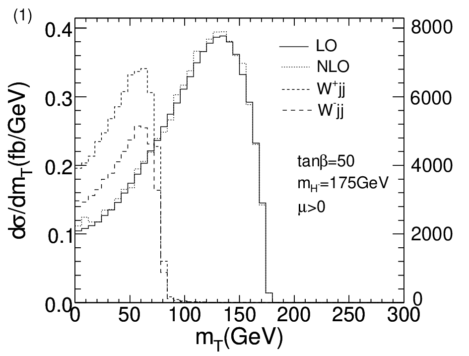
Our simulation results for the relevant distributions are shown in Figs. 12-16, which include the distributions of the $m_{T}$ , the $p_{T}$ for all jets and the missing transverse momentum for the signal and backgrounds after the basic cuts, assuming: (1) $m_{0}=\ 200{\rm GeV},m_{1/2}=147\ {\rm GeV},A_{0}=200\ {\rm GeV},\tan\beta=50$ and $\mu>0$ ; (2) $m_{0}=320\ {\rm GeV},m_{1/2}=400\ {\rm GeV},A_{0}=300\ {\rm GeV},\tan\beta=50$ and $\mu>0$ . In case (1) of those figures, the NLO QCD corrections can be neglected for all the distributions, but in case (2), the NLO QCD corrections reduce the LO results significantly, which can reach above 10% in some region of the distributions. It can be seen that the additional cuts introduced at the LO still work well when including the NLO QCD effects.

In the following calculations of the total cross sections the additional cuts are used. Moreover, an integrated luminosity of $300\ {\rm fb}^{-1}$ and a $\tau$ detection efficiency of $30\%$ are taken to calculate the significance $S/\sqrt{B}$ . The total cross sections for the backgrounds from the final state $W^{+}+2j$ and $W^{-}+2j$ are about 32 fb and 25 fb, respectively. Now, we add the cross sections of the $H^{-}W^{+}$ and the $H^{+}W^{-}$ production together, as well as for the backgrounds. Tables 2 and 3 show some representative results of the cross sections and the significance, where we can see that the significance can reach above 20 for $\tan\beta=50$ and $m_{H^{-}}=175\ \rm{GeV}$ .

	Integrated cross section (fb)
Parameter	Signal Background $S/\sqrt{B}$
$m_{H^{-}}=175{\rm GeV}$	LO 17.6 57 22.1
	NLO 17.2 57 21.6
$m_{H^{-}}=345{\rm GeV}$	LO 2.12 57 2.66
	NLO 1.84 57 2.31
$m_{H^{-}}=630{\rm GeV}$	LO 0.34 57 0.43
	NLO 0.28 57 0.35

Table 2: Results under several groups of

m_{H^{-}}

value, assuming

m_{0}=A_{0}=200\ {\rm GeV}

, and

\tan\beta=50

	Integrated cross section (fb)
Parameter	Signal Background $S/\sqrt{B}$
$\tan\beta=20$	LO 0.46 57 0.58
	NLO 0.42 57 0.53
$\tan\beta=40$	LO 4.60 57 5.78
	NLO 4.34 57 5.45
$\tan\beta=50$	LO 17.7 57 22.3
	NLO 16.7 57 21.0

Table 3: Results under several groups of

\tan\beta

value, assuming

m_{0}=A_{0}=200\ {\rm GeV}

, and

m_{1/2}=150\ {\rm GeV}

. The three

\tan\beta

values correspond to

m_{H^{\pm}}=282\ {\rm GeV}

224\ {\rm GeV}

and

178\ {\rm GeV}

from top to bottom, respectively.

Figs. 17 and 18 show the dependence of the cross sections on $m_{H^{-}}$ mass and $\tan\beta$ , respectively. In general, the NLO QCD corrections reduce the cross sections in most of the parameter space, and their magnitude can be larger than 10%. The horizontal lines in the figures correspond to the total cross sections required for $S/\sqrt{B}=5$ . It can be seen that at the LO the signal can be detected at a $5\sigma$ level for $\tan\beta\gtrsim 40$ and $m_{1/2}=150\ {\rm GeV}$ , and for $100\ {\rm GeV}\lesssim m_{H^{-}}\lesssim 250\ {\rm GeV}$ and $\tan\beta=50$ , respectively. And the NLO QCD corrections have small effects on the above results. Some of our results are different from those given in Ref. Eriksson et al. 2006 mainly due to the difference between the mSUGRA scenario and the one used in Ref. Eriksson et al. 2006.

VI CONCLUSIONS

In conclusion, we have calculated the NLO QCD corrections to the inclusive total cross sections of the $H^{\mp}W^{\pm}$ pairs produced at the LHC through $b\bar{b}$ annihilation in the MSSM. The NLO QCD corrections can either enhance or reduce the total cross sections, but they generally efficiently reduce the dependence of the total cross sections on the renormalization/factorization scale. The magnitude of the NLO QCD corrections is about 10% in most of the parameter space and can reach 15% in some parameter region. Finally, we give some discussion on the $H^{\mp}W^{\pm}\to 2j+\tau_{jet}+\not{\!p}_{T}$ signal including the NLO QCD effects, and find an observable signal at a $5\sigma$ level in some region of the mSUGRA parameter space.

Acknowledgements.

This work was supported in part by the National Natural Science Foundation of China, under Grants No.10421503, No.10575001 and No.10635030 and the Key Grant Project of Chinese Ministry of Education under Grant No.305001.

APPENDIX

In this appendix, we give the relevant Feynman rules and the form factors for the virtual amplitude. First we give the relevant Feynman rules.
1. $h^{0}(H^{0})-b-\bar{b}:\quad{\mathcal{A}}_{1(2)}m_{b}$

{\mathcal{A}}_{1}=\frac{ie\delta_{ij}s_{\alpha}}{2c_{\beta}M_{W}s_{W}},\quad{\mathcal{A}}_{2}=\frac{-ie\delta_{ij}c_{\alpha}}{2c_{\beta}M_{W}s_{W}},

where $\alpha$ is the mixing angle in the CP even neutral Higgs boson sector. Here we use the abbreviations $s_{\alpha}=\sin\alpha$ , $s_{\beta}=\sin\beta$ and so on.
2. $A^{0}-b-\bar{b}:\quad{\mathcal{A}}_{3}m_{b}\gamma_{5}$

{\mathcal{A}}_{3}=\frac{-e\delta_{ij}t_{\beta}}{2M_{W}s_{W}}.

3. $h^{0}(H^{0},A^{0})-W^{-}-H^{+}:\quad{\mathcal{F}}_{1(2,3)}(p_{h^{0}(H^{0},A^{0})}-p_{H^{+}})^{\mu}$

{\mathcal{F}}_{1}=\frac{iec_{\beta-\alpha}}{2s_{W}},\quad{\mathcal{F}}_{2}=-\frac{ies_{\beta-\alpha}}{2s_{W}},\quad{\mathcal{F}}_{3}=\frac{e}{2s_{W}}.

Here we define the ingoing four-momenta to be positive.
4. $b-\bar{t}-H^{+}:\quad{\mathcal{G}}_{1}P_{L}+{\mathcal{G}}_{2}P_{R}$

{\mathcal{G}}_{1}=\frac{ie\delta_{ij}m_{t}}{\sqrt{2}M_{W}s_{W}t_{\beta}},\quad{\mathcal{G}}_{2}=\frac{ie\delta_{ij}m_{b}t_{\beta}}{\sqrt{2}M_{W}s_{W}}.

Here and below, we assume the third generation CKM matrix element $V_{tb}$ equal to 1.
5. $\bar{b}-t-W^{-}:\quad{\mathcal{G}}_{3}\gamma^{\mu}P_{L}$

{\mathcal{G}}_{3}=\frac{-ie}{\sqrt{2}s_{W}}.

Below we collect the explicit expressions of the nonzero form factors in Eq.(10). For simplicity, we introduce the following abbreviations for the Passarino-Veltman two-point integrals $B_{i(j)}$ , three-point integrals $C_{i(j)}$ and four-point integrals $D_{i(j)}$ , which are defined similar to Ref. Denner 1993 except that we take internal masses squared as arguments:
$B^{a}_{i(j)}=B_{i(j)}(s,0,0)$ ,
$B^{b}_{i(j)}=B_{i(j)}(t,0,m_{t}^{2})$ ,
$C^{a}_{i,(j)}=C_{i(j)}(M_{H^{-}}^{2},0,t,m_{t}^{2},0,0)$ ,
$C^{b}_{i,(j)}=C_{i(j)}(M_{W}^{2},0,t,m_{t}^{2},0,0)$ ,
$C^{c}_{i,(j)}=C_{i(j)}(0,s,0,0,0,0)$ ,
$C^{d}_{i,(j)}=C_{i(j)}(0,t,M_{H^{-}}^{2},0,0,m_{t}^{2})$ ,
$C^{e}_{i,(j)}=C_{i(j)}(0,t,M_{W}^{2},0,0,m_{t}^{2})$ ,
$D_{i(j)}=D_{i(j)}(M_{W}^{2},s,0,t,M_{H^{-}}^{2},0,m_{t}^{2},0,0,0)$ .
Most of the above functions contain IR singularities. Since all the Passarino-Veltman integrals can be written as a combination of the scalar functions $A_{0},B_{0},C_{0}$ and $D_{0}$ , we present here the explicit expressions for the $C_{0}$ and $D_{0}$ functions, which contain the IR divergences and were used in our calculations:
$\displaystyle{C^{c}_{0}=\frac{C_{\epsilon}}{s}\left[\frac{1}{\epsilon^{2}}-\frac{\pi^{2}}{3}\right],}$
$\displaystyle{C^{a}_{0}=C^{d}_{0}=\frac{C_{\epsilon}}{t-M_{H^{-}}^{2}}\left[\frac{1}{\epsilon}\ln\frac{m_{t}^{2}-M_{H^{-}}^{2}}{m_{t}^{2}-t}+{\rm Li}\left(\frac{M_{H^{-}}^{2}}{M_{H^{-}}^{2}-m_{t}^{2}}\right)-{\rm Li}\left(\frac{t}{t-m_{t}^{2}}\right)\right.}$
$\displaystyle{\qquad\left.-\frac{1}{2}\ln^{2}(m_{t}^{2}-M_{H^{-}}^{2})+\frac{1}{2}\ln^{2}(m_{t}^{2}-t)+\ln s\ln\frac{m_{t}^{2}-M_{H^{-}}^{2}}{m_{t}^{2}-t}\right],}$
$\displaystyle{C^{e}_{0}=C^{b}_{0}=C^{a}_{0}(M_{W}^{2}\leftrightarrow M_{H^{-}}^{2}),}$
$\displaystyle{D_{0}=\frac{C_{\epsilon}}{s(t-m_{t}^{2})}\left[\frac{1}{\epsilon^{2}}-\frac{1}{\epsilon}\ln\frac{(t-m_{t}^{2})^{2}}{(m_{t}^{2}-M_{H^{-}}^{2})(m_{t}^{2}-M_{W}^{2})}\right.}$
$\displaystyle{\qquad-\ln s\ln\frac{(t-m_{t}^{2})^{2}}{(m_{t}^{2}-M_{H^{-}}^{2})(m_{t}^{2}-M_{W}^{2})}-2{\rm Li}\left(1+\frac{m_{t}^{2}-M_{W}^{2}}{t-m_{t}^{2}}\right)-2{\rm Li}\left(1+\frac{m_{t}^{2}-M_{H^{-}}^{2}}{t-m_{t}^{2}}\right)}$
$\displaystyle{\qquad-{\rm Li}\left[1+\frac{(m_{t}^{2}-M_{H^{-}}^{2})(m_{t}^{2}-M_{W}^{2})}{sm_{t}^{2}}\right]-\frac{1}{2}\ln^{2}\left(\frac{s}{m_{t}^{2}}\right)+2\ln s\ln\left(\frac{t-m_{t}^{2}}{m_{t}^{2}}\right)}$
$\displaystyle{\qquad\left.-\ln(m_{t}^{2}-M_{H^{-}}^{2})\ln\left(\frac{m_{t}^{2}-M_{H^{-}}^{2}}{m_{t}^{2}}\right)-\ln(m_{t}^{2}-M_{W}^{2})\ln\left(\frac{m_{t}^{2}-M_{W}^{2}}{m_{t}^{2}}\right)\right],}$
where $C_{\epsilon}=(4\pi\mu_{r}^{2}/s)^{\epsilon}\Gamma(1-\epsilon)/\Gamma(1-2\epsilon)$ . For diagrams(a)-(f) in Fig.2, we get the form factors as following, respectively,
$\displaystyle{f_{5}^{a}=f_{6}^{a}=f_{9}^{a}=f_{10}^{a}=C_{F}\delta_{ij}\frac{\alpha_{s}}{4\pi}\frac{e^{2}m_{b}s_{\alpha}c_{\beta-\alpha}}{c_{\beta}M_{W}s_{W}^{2}(s-m_{h^{0}}^{2})}\left[(C_{0}^{c}+C_{1}^{c}+C_{2}^{c})s-2B_{0}^{a}\right],}$
$\displaystyle{f_{5}^{b}=f_{6}^{b}=f_{9}^{b}=f_{10}^{b}=C_{F}\delta_{ij}\frac{\alpha_{s}}{4\pi}\frac{e^{2}m_{b}c_{\alpha}s_{\beta-\alpha}}{c_{\beta}M_{W}s_{W}^{2}(s-m_{H^{0}}^{2})}\left[(C_{0}^{c}+C_{1}^{c}+C_{2}^{c})s-2B_{0}^{a}\right],}$
$\displaystyle{f_{5}^{c}=f_{9}^{c}=-f_{6}^{c}=-f_{10}^{c}=C_{F}\delta_{ij}\frac{\alpha_{s}}{4\pi}\frac{e^{2}m_{b}t_{\beta}}{M_{W}s_{W}^{2}(s-m_{A^{0}}^{2})}\left[(C_{0}^{c}+C_{1}^{c}+C_{2}^{c})s-2B_{0}^{a}\right],}$
$\displaystyle{f_{2}^{d}=-C_{F}\delta_{ij}\frac{\alpha_{s}}{2\pi}\frac{e}{\sqrt{2}s_{W}(t-m_{t}^{2})^{2}}(2m_{t}a)(tB^{b}_{1}-m_{t}^{2}B^{b}_{0}),}$
$\displaystyle{f_{9}^{d}=2f_{3}^{d}=-C_{F}\delta_{ij}\frac{\alpha_{s}}{2\pi}\frac{e}{\sqrt{2}s_{W}(t-m_{t}^{2})^{2}}(-2b)[m_{t}^{2}(B^{b}_{1}-3B^{b}_{0})+t(B^{b}_{0}+B^{b}_{1})],}$
$\displaystyle{f_{2}^{e}=C_{F}\delta_{ij}\frac{\alpha_{s}}{4\pi}\frac{e}{\sqrt{2}s_{W}(t-m_{t}^{2})}(am_{t})\left[4B_{0}^{b}+2(M_{H^{-}}^{2}-t)C_{1}^{d}+2(2M_{H^{-}}^{2}-t)C_{2}^{d}\right],}$
$\displaystyle{f_{9}^{e}=2f_{3}^{e}=C_{F}\delta_{ij}\frac{\alpha_{s}}{4\pi}\frac{e}{\sqrt{2}s_{W}(t-m_{t}^{2})}(-2b)\left[4B_{0}^{b}+2(M_{H^{-}}^{2}-t)C_{1}^{d}+2(2M_{H^{-}}^{2}-m_{t}^{2})C_{2}^{d}\right],}$
$\displaystyle{f_{2}^{f}=C_{F}\delta_{ij}\frac{\alpha_{s}}{4\pi}\frac{e}{\sqrt{2}s_{W}(t-m_{t}^{2})}(2am_{t})\left[2C_{00}^{e}+M_{W}^{2}(C_{2}^{e}+C_{22}^{e})+(M_{W}^{2}-t)(C_{1}^{e}+C_{12}^{e})\right],}$
$\displaystyle{f_{3}^{f}=C_{F}\delta_{ij}\frac{\alpha_{s}}{4\pi}\frac{e}{\sqrt{2}s_{W}(t-m_{t}^{2})}(-2b)\left[2C_{00}^{e}+M_{W}^{2}(C_{2}^{e}+C_{22}^{e})+(M_{W}^{2}-t)(C_{1}^{e}+C_{12}^{e})\right],}$
$\displaystyle{f_{9}^{f}=C_{F}\delta_{ij}\frac{\alpha_{s}}{4\pi}\frac{e}{\sqrt{2}s_{W}(t-m_{t}^{2})}(-4b)\left[2C_{00}^{e}+M_{W}^{2}(C_{1}^{e}+C_{2}^{e}+C_{12}^{e}+C_{22}^{e})-m_{t}^{2}C_{1}^{e}\right],}$
$\displaystyle{f_{12}^{f}=C_{F}\delta_{ij}\frac{\alpha_{s}}{4\pi}\frac{e}{\sqrt{2}s_{W}(t-m_{t}^{2})}C_{12}^{e},}$
where a,b are abbreviations for

a=\frac{em_{t}}{\sqrt{2}M_{W}s_{W}t_{\beta}},\qquad b=\frac{em_{b}t_{\beta}}{\sqrt{2}M_{W}s_{W}}.

For the box diagram(g) in Fig.2, we find
$\displaystyle{f_{2}^{box}=C_{F}\delta_{ij}\frac{\alpha_{s}}{4\pi}\frac{e}{\sqrt{2}s_{W}}(-2m_{t}a)\left\{\left[-2D_{00}-M_{W}^{2}(D_{11}+D_{13}+D_{1}+D_{3})\right.\right.}$
$\displaystyle{\left.\left.\qquad-M_{H^{-}}^{2}(D_{2}+D_{3}+D_{22}+D_{23})\right]-(D_{12}+D_{13}+D_{23}+D_{33})t-(D_{12}+D_{0}+D_{1}+D_{2})u\right\},}$
$\displaystyle{f_{3}^{box}=C_{F}\delta_{ij}\frac{\alpha_{s}}{4\pi}\frac{e}{\sqrt{2}s_{W}}(-2b)D_{3}s,}$
$\displaystyle{f_{5}^{box}=C_{F}\delta_{ij}\frac{\alpha_{s}}{4\pi}\frac{e}{\sqrt{2}s_{W}}(4b)\left[-C^{a}_{0}+M^{2}_{W}(D_{0}+D_{1}+D_{2}+D_{3})-D_{2}s\right],}$
$\displaystyle{f_{8}^{box}=C_{F}\delta_{ij}\frac{\alpha_{s}}{4\pi}\frac{e}{\sqrt{2}s_{W}}(-2m_{t}a)\left[-2(D_{0}+D_{1}+2D_{2}+D_{3}+D_{12}+D_{22}+D_{23})\right],}$
$\displaystyle{f_{9}^{box}=C_{F}\delta_{ij}\frac{\alpha_{s}}{4\pi}\frac{e}{\sqrt{2}s_{W}}(4b)\left[C_{2}^{b}-C_{0}^{a}+M_{W}^{2}(D_{0}+D_{1})+(t+u-M^{2}_{H^{-}})D_{2}+(t+u)D_{3}\right],}$
$\displaystyle{f_{12}^{box}=C_{F}\delta_{ij}\frac{\alpha_{s}}{4\pi}\frac{e}{\sqrt{2}s_{W}}(-2m_{t}a)\left[-2(D_{2}+D_{3}+D_{12}+D_{13}+D_{22}+2D_{23}+D_{33})\right].}$

References

Higgs (1964) P. W. Higgs, Phys. Lett. 12, 132 (1964); F. Englert and R. Brout, Phys. Rev. Lett. 13, 321 (1964); G. S. Guralnik, C. R. Hagen, and T. W. B. Kibble, Phys. Rev. Lett. 13, 585 (1964); P. W. Higgs, Phys. Rev. 145, 1156 (1966).
Nilles (1984) H. P. Nilles, Phys. Rept. 110, 1 (1984); H. E. Haber and G. L. Kane, Phys. Rept. 117, 75 (1985); A. B. Lahanas and D. V. Nanopoulos, Phys. Rept. 145, 1 (1987).
Bawa et al. (1990) A. C. Bawa, C. S. Kim, and A. D. Martin, Z. Phys. C47, 75 (1990); L. G. Jin, C. S. Li, R. J. Oakes, and S. H. Zhu, Eur. Phys. J. C14, 91 (2000); T. Plehn, Phys. Rev. D67, 014018 (2003); S.-h. Zhu, Phys. Rev. D67, 075006 (2003); E. L. Berger, T. Han, J. Jiang, and T. Plehn, Phys. Rev. D71, 115012 (2005); N. Kidonakis, PoS HEP2005, 336 (2006); Y.-B. Liu and J.-F. Shen (2007), eprint arXiv:0704.0840 [hep-ph].
Moretti and Odagiri (1997) S. Moretti and K. Odagiri, Phys. Rev. D55, 5627 (1997).
Hesselbach et al. (2007) S. Hesselbach, S. Moretti, J. Rathsman, and A. Sopczak (2007), eprint arXiv:0708.4394 [hep-ph].
Eichten et al. (1984) E. Eichten, I. Hinchliffe, K. D. Lane, and C. Quigg, Rev. Mod. Phys. 56, 579 (1984); N. G. Deshpande, X. Tata, and D. A. Dicus, Phys. Rev. D29, 1527 (1984); A. Krause, T. Plehn, M. Spira, and P. M. Zerwas, Nucl. Phys. B519, 85 (1998); A. A. Barrientos Bendezu and B. A. Kniehl, Nucl. Phys. B568, 305 (2000); O. Brein and W. Hollik, Eur. Phys. J. C13, 175 (2000).
Dicus et al. (1989) D. A. Dicus, J. L. Hewett, C. Kao, and T. G. Rizzo, Phys. Rev. D40, 787 (1989).
Barrientos Bendezu and Kniehl (2001) A. A. Barrientos Bendezu and B. A. Kniehl, Phys. Rev. D63, 015009 (2001); O. Brein, W. Hollik, and S. Kanemura, Phys. Rev. D63, 095001 (2001).
Yang et al. (2000) Y.-S. Yang, C.-S. Li, L.-G. Jin, and S. H. Zhu, Phys. Rev. D62, 095012 (2000).
Hollik and Zhu (2002) W. Hollik and S.-h. Zhu, Phys. Rev. D65, 075015 (2002).
Zhao et al. (2005) J. Zhao, C. S. Li, and Q. Li, Phys. Rev. D72, 114008 (2005).
Bern et al. (2002) Z. Bern, A. De Freitas, L. J. Dixon, and H. L. Wong, Phys. Rev. D66, 085002 (2002).
Ellis et al. (2001) J. R. Ellis, D. V. Nanopoulos, and K. A. Olive, Phys. Lett. B508, 65 (2001).
Aivazis et al. (1994) M. A. G. Aivazis, J. C. Collins, F. I. Olness, and W.-K. Tung, Phys. Rev. D50, 3102 (1994); J. C. Collins, Phys. Rev. D58, 094002 (1998); M. Kramer, F. I. Olness, and D. E. Soper, Phys. Rev. D62, 096007 (2000).
Eriksson et al. (2006) D. Eriksson, S. Hesselbach, and J. Rathsman (2006), eprint hep-ph/0612198.
Drees and Martin (1995) M. Drees and S. P. Martin (1995), eprint hep-ph/9504324.
Denner (1993) A. Denner, Fortschr. Phys. 41, 307 (1993).
Altarelli et al. (1979) G. Altarelli, R. K. Ellis, and G. Martinelli, Nucl. Phys. B157, 461 (1979).
Harris and Owens (2002) B. W. Harris and J. F. Owens, Phys. Rev. D65, 094032 (2002).
Collins et al. (1985) J. C. Collins, D. E. Soper, and G. Sterman, Nucl. Phys. B261, 104 (1985); G. T. Bodwin, Phys. Rev. D31, 2616 (1985).
Altarelli and Parisi (1977) G. Altarelli and G. Parisi, Nucl. Phys. B126, 298 (1977).
Ellis et al. (1981) R. K. Ellis, D. A. Ross, and A. E. Terrano, Nucl. Phys. B178, 421 (1981); Z. Kunszt and D. E. Soper, Phys. Rev. D46, 192 (1992); M. L. Mangano, P. Nason, and G. Ridolfi, Nucl. Phys. B373, 295 (1992).
Beenakker et al. (1997) W. Beenakker, R. Hopker, M. Spira, and P. M. Zerwas, Nucl. Phys. B492, 51 (1997).
Sjostrand et al. (2001) T. Sjostrand, L. Lonnblad, and S. Mrenna (2001), eprint hep-ph/0108264.
Jadach et al. (1990) S. Jadach, J. H. Kuhn, and Z. Was, Comput. Phys. Commun. 64, 275 (1990).
Golonka et al. (2006) P. Golonka et al., Comput. Phys. Commun. 174, 818 (2006).
Mangano et al. (2003) M. L. Mangano, M. Moretti, F. Piccinini, R. Pittau, and A. D. Polosa, JHEP 07, 001 (2003).
Yao et al. (2006) W. M. Yao et al. (Particle Data Group), J. Phys. G33, 1 (2006).
Gorishnii et al. (1990) S. G. Gorishnii, A. L. Kataev, S. A. Larin, and L. R. Surguladze, Mod. Phys. Lett. A5, 2703 (1990); S. G. Gorishnii, A. L. Kataev, S. A. Larin, and L. R. Surguladze, Phys. Rev. D43, 1633 (1991); A. Djouadi, M. Spira, and P. M. Zerwas, Z. Phys. C70, 427 (1996); A. Djouadi, J. Kalinowski, and M. Spira, Comput. Phys. Commun. 108, 56 (1998); M. Spira, Fortsch. Phys. 46, 203 (1998).
Pumplin et al. (2002) J. Pumplin et al., JHEP 07, 012 (2002).
Carena et al. (2000) M. S. Carena, D. Garcia, U. Nierste, and C. E. M. Wagner, Nucl. Phys. B577, 88 (2000).
Porod (2003) W. Porod, Comput. Phys. Commun. 153, 275 (2003).

Refer to caption — Figure 1: Leading order Feynman diagrams for $b\bar{b}\to H^{-}W^{+}$ .