The Boltzmann-Grad limit of the periodic Lorentz gas in two space dimensionsJournal: the Académie des sciences

On appelle gaz de Lorentz le système dynamique correspondant au mouvement libre d’une particule ponctuelle dans un système d’obstacles circulaires de rayon $r$ centrés aux sommets d’un réseau de $\mathbf{R}^{2}$, supposant que les collisions entre la particule et les obstacles sont parfaitement élastiques. Les trajectoires de la particule sont alors données par les formules (2). La limite de Boltzmann-Grad pour le gaz de Lorentz consiste à supposer que le rayon des obstacles $r\to 0^{+}$, et à observer la dynamique de la particule sur des plages de temps longues, de l’ordre de $1/r$ — voir (3) pour la loi d’échelle de Boltzmann-Grad en dimension $2$.

Or les trajectoires de la particule s’expriment en fonction de l’application de transfert d’obstacle à obstacle $T_{r}$ définie par (8) — où la notation $Y$ désigne la transformation inverse de (7) — application qui associe, à tout paramètre d’impact $h^{\prime}\in[-1,1]$ correspondant à une particule quittant la surface d’un obstacle dans la direction $\omega\in\mathbf{S}^{1}$, le paramètre d’impact $h$ à la collision suivante, ainsi que le temps $s$ s’écoulant jusqu’à cette collision. (Pour une définition de la notion de paramètre d’impact, voir (6).)

On se ramène donc à étudier le comportement limite de l’application de transfert $T_{r}$ pour $r\to 0^{+}$.

Les paramètres $A,B,Q,N\,\hbox{Êmod. }2$ intervenant dans l’application de transfert asymptotique sont définis à partir du développement en fraction continue (9) de $\alpha$ par les formules (11) et (12).

On voit sur ces formules que les paramètres $A,B,Q,N\,\hbox{Êmod. }2$ sont des fonctions très fortement oscillantes des variables $\omega$ et $r$. Il est donc naturel de chercher le comportement limite de l’application de transfert $T_{r}$ dans une topologie faible vis à vis de la dépendance en la direction $\omega$. On montre ainsi que, pour tout $h^{\prime}\in[-1,1]$, la famille d’applications $\omega\mapsto T_{r}(h^{\prime},\omega)$ converge au sens des mesures de Young (voir par exemple [8] p. 146–154 pour une définition de cette notion) lorsque $r\to 0^{+}$ vers une mesure de probabilité $P(s,h|h^{\prime})dsdh$ indépendante de $\omega$ :

Le théorème ci-dessus est le résultat principal de cette Note : il montre que, dans la limite de Boltzmann-Grad, le transfert d’obstacle à obstacle est décrit de manière naturelle par une densité de probabilité de transition $P(s,h|h^{\prime})$, où $s$ est le laps de temps entre deux collisions successives avec les obstacles (dans l’échelle de temps de la limite de Boltzmann-Grad), $h$ le paramètre d’impact lors de la collision future et $h^{\prime}$ celui correspondant à la collision passée.

Le fait que la probabilité de transition $P(s,h|h^{\prime})$ soit indépendante de la direction suggère l’hypothèse d’indépendance (H) des quantités $A,B,Q,N\,\hbox{Êmod. 2}$ correspondant à des collisions successives.

Dans le cas d’obstacles aléatoires indépendants et poissonniens, Gallavotti a montré que la limite de Boltzmann-Grad du gaz de Lorentz obéit à l’équation cinétique de Lorentz (4). Le cas périodique est absolument différent : en se basant sur des estimations (cf. [3] et [7]) du temps de sortie du domaine $Z_{r}$ défini dans (1), on démontre que la limite de Boltzmann-Grad du gaz de Lorentz périodique ne peut pas être décrite par l’équation de Lorentz (4) sur l’espace des phases $\mathbf{R}^{2}\times\mathbf{S}^{1}$ classique de la théorie cinétique : voir [6]. Si l’hypothèse (H) ci-dessous était vérifiée, le modèle cinétique (22) dans l’espace des phases étendu fournirait donc l’équation devant remplacer l’équation cinétique classique de Lorentz (4) dans le cas périodique.

The Lorentz gas is the dynamical system corresponding to the free motion of a single point particle in a periodic system of fixed spherical obstacles, assuming that collisions between the particle and any of the obstacles are elastic. Henceforth, we assume that the space dimension is $2$ and that the obstacles are disks of radius $r$ centered at each point of $\mathbf{Z}^{2}$. Hence the domain left free for particle motion is

Assuming that the particle moves at speed $1$, its trajectory starting from $x\in Z_{r}$ with velocity $\omega\in\mathbf{S}^{1}$ at time $t=0$ is $t\mapsto(X_{r},\Omega_{r})(t;x,\omega)\in\mathbf{R}^{2}\times\mathbf{S}^{1}$ given by

denoting $\dot{}=\frac{d}{dt}$ and $\mathcal{R}[X_{r}(t)]$ the specular reflection on $\partial Z_{r}$ at the point $X_{r}(t)=X_{r}(t\pm 0)$. Assume that the initial position $x$ and direction $\omega$ of the particle are distributed in $Z_{r}\times\mathbf{S}^{1}$ with some probability density $f^{in}\equiv f^{in}(x,\omega)$, and define

We are concerned with the limit of $f_{r}$ as $r\to 0^{+}$ in some appropriate sense to be explained below. In the 2-dimensional setting considered here, this is precisely the Boltzmann-Grad limit.

In the case of a random (Poisson), instead of periodic, configuration of obstacles, Gallavotti [5] proved that the expectation of $f_{r}$ converges to the solution of the Lorentz kinetic equation for $(x,\omega)\in\mathbf{R}^{2}\times\mathbf{S}^{1}$:

In the case of a periodic distribution of obstacles, the Boltzmann-Grad limit of the Lorentz gas cannot be described by a transport equation as above: see [6] for a complete proof, based on estimates on the free path length to be found in [3] and [7]. This limit involves instead a linear Boltzmann equation on an extended phase space with two new variables taking into account correlations between consecutive collisions with the obstacles that are an effect of periodicity: see Theorem 4.1.

Denote by $n_{x}$ the inward unit normal to $Z_{r}$ at the point $x\in\partial Z_{r}$, consider

and let $\Gamma^{\pm}_{r}/\mathbf{Z}^{2}$ be the quotient of $\Gamma^{\pm}_{r}$ under the action of $\mathbf{Z}^{2}$ by translation on the $x$ variable. For $(x,\omega)\in\Gamma^{+}_{r}$, let $\tau_{r}(x,\omega)$ be the exit time from $x$ in the direction $\omega$ and $h_{r}(x,\omega)$ be the impact parameter:

Obviously, the map

coordinatizes $\Gamma^{+}_{r}/\mathbf{Z}^{2}$, and we henceforth denote $Y_{r}$ its inverse.

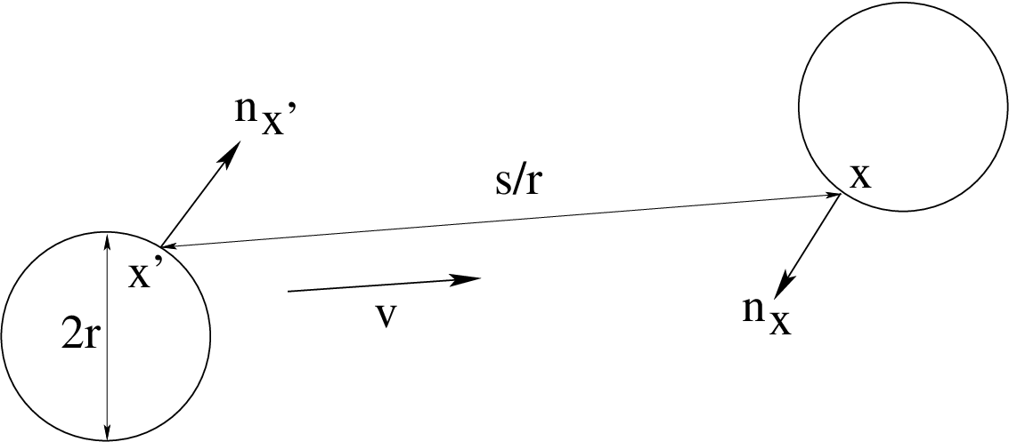
For each $r\in]0,\frac{1}{2}[$, consider now the transfer map $T_{r}:\,]-1,1[\times\mathbf{S}^{1}\to\mathbf{R}_{+}^{*}\times]-1,1[$ defined by

For a particle leaving the surface of an obstacle in the direction $\omega$ with impact parameter $h^{\prime}$, the transition map $T_{r}(h^{\prime},\omega)=(s,h)$ gives the (rescaled) distance $s$ to the next collision, and the corresponding impact parameter $h$. Obviously, each trajectory (2) of the particle can be expressed in terms of the transfer map $T_{r}$ and iterates thereof. The Boltzmann-Grad limit of the periodic Lorentz gas is therefore reduced to computing the limiting behavior of $T_{r}$ as $r\to 0^{+}$, and this is our main purpose in this Note.

We first need some pieces of notation. Assume $\omega=(\omega_{1},\omega_{2})$ with $0<\omega_{2}<\omega_{1}$, and $\alpha=\omega_{2}/\omega_{1}\in]0,1[\setminus\mathbf{Q}$. Consider the continued fraction expansion of $\alpha$:

Define the sequences of convergents $(p_{n},q_{n})_{n\geq 0}$ and errors $(d_{n})_{n\geq 0}$ by the recursion formulas

and let

The proof uses the 3-term partition of the 2-torus defined in section 2 of [4], following the work of [1].

For $\omega=(\cos\theta,\sin\theta)$ with arbitrary $\theta\in\mathbf{R}$, the map $h^{\prime}\mapsto T_{r}(h^{\prime},\omega)$ is computed using Proposition 2.1 in the following manner. Set $\tilde{\theta}=\theta-m\frac{\pi}{2}$ with $m=[\frac{2}{\pi}(\theta+\frac{\pi}{4})]$ and let $\tilde{\omega}=(\cos\tilde{\theta},\sin\tilde{\theta})$. Then

The formulas (11) and (12) defining $A,B,Q,N\,\hbox{Êmod. 2}$ show that these quantities are strongly oscillating functions of the variables $\omega$ and $r$. In view of Proposition 2.1, one therefore expects the transfer map $T_{r}$ to have a limit as $r\to 0^{+}$ only in the weakest imaginable sense, i.e. in the sense of Young measures — see [8], pp. 146–154 for a definition of this notion of convergence.

The main result in the present Note is the theorem below. It says that, for each $h^{\prime}\in[-1,1]$, the family of maps $\omega\mapsto T_{r}(h^{\prime},\omega)$ converges as $r\to 0^{+}$ and in the sense of Young measures to some probability measure $P(s,h|h^{\prime})dsdh$ that is moreover independent of $\omega$.

The proof of (16-17) is based on the explicit representation of the transition map in Proposition 2.1 together with Kloosterman sums techniques as in [2]. The explicit formula for the transition probability $P$ is very complicated and we do not report it here, however it clearly entails the properties (18).

For each $r\in]0,\frac{1}{2}[$, denote $d\gamma^{+}_{r}(x,\omega)$ the probability measure on $\Gamma^{+}_{r}$ that is proportional to $\omega\cdot n_{x}dxd\omega$. This probability measure is invariant under the billiard map

For $(x^{0},\omega^{0})\in\Gamma^{+}_{r}$, set $(x^{n},\omega^{n})=\mathbf{B}^{n}_{r}(x^{0},\omega^{0})$ and $\alpha^{n}=\min(|\omega^{n}_{1}/\omega^{n}_{2}|,|\omega^{n}_{2}/\omega^{n}_{1}|)$ for each $n\geq 0$, and define

We make the following asymptotic independence hypothesis: for each $n\geq 1$ and each $\Psi\in C([-1,1]\times K^{n})$

Under this assumption, the Boltzmann-Grad limit of the Lorentz gas is described by a kinetic model on the extended phase space $\mathbf{R}^{2}\times\mathbf{S}^{1}\times\mathbf{R}_{+}\times[-1,1]$ — unlike the Lorentz kinetic equation (4), that is set on the usual phase space $\mathbf{R}^{2}\times\mathbf{S^{1}}$.

For each $(s_{0},h_{0})\in\mathbf{R}_{+}\times[-1,1]$, let $(s_{n},h_{n})_{n\geq 1}$ be the Markov chain defined by the induction formula

where $\beta_{n}\in K$ are independent random variables distributed under $\mu$. The proof of Theorem 4.1 relies upon approximating the particle trajectory $(X_{r},\Omega_{r})(t)$ starting from $(x_{0},\omega_{0})$ in terms of the following jump process with values in $\mathbf{R}^{2}\times\mathbf{S^{1}}\times\mathbf{R}_{+}\times[-1,1]$ with the help of Proposition 2.1

Unlike in the case of a random (Poisson) distribution of obstacles, the successive impact parameters on each particle path are not independent and uniformly distributed in the periodic case — likewise, the successive free path lengths on each particle path are not independent with exponential distribution. The Markov chain (23) is introduced to handle precisely this difficulty.