MS-TP-07-28
Strong coupling expansion for Yang-Mills theory at finite temperature

The partition function of the lattice Yang-Mills theory is given by a functional integration of the exponentiated Wilson action over the corresponding SU(N) group space,

	$\displaystyle Z$	$\displaystyle=$	$\displaystyle\int\,DU\,\exp\left[\sum_{p}\frac{\beta}{2N}\left(\mathrm{Tr}\,U+\mathrm{Tr}\,U^{\dagger}-2N\right)\right],$		(1)
	$\displaystyle\beta$	$\displaystyle=$	$\displaystyle\frac{2N}{g^{2}}.$

An expansion in the lattice coupling $\beta$ by group characters $\chi_{r}(U)$ and a cluster expansion yields the free energy density [1]

$$\tilde{f}\equiv-\frac{1}{\Omega}\ln Z=-6\ln\,c_{0}(\beta)-\frac{1}{\Omega}\sum_{C=(X_{i}^{n_{i}})}\,a(C)\prod_{i}\Phi(X_{i})^{n_{i}}.$$

(2)

where $\Omega=V\cdot N_{t}$ is the lattice volume and $c_{0}$ is the expansion coefficient of the trivial representation, which has been factored out. The combinatorial factor $a(C)$ is introduced via a moment-cumulant-formalism, and equals $1$ for clusters $C$ which consist of only one so-called polymer $X_{i}$. The quantity in equation (2) is customarily called a free energy, even at zero physical temperature, because the path integral corresponds to a partition function if one formally identifies $\beta$ with $1/T$. Here we are interested in a physical temperature $T=1/(aN_{t})$, realized by compactifying the temporal extension of the lattice. The physical free energy is then obtained by subtracting the formal ($N_{t}=\infty$) free energy, which is analogous to a subtraction of the divergent vacuum energy in the continuum. Thus the physical free energy density reads

$$f(N_{t},u)=\tilde{f}(N_{t},u)-\tilde{f}(\infty,u).$$

(3)

The contributing polymers $X_{i}$ have to be objects with a closed surface, since

$\displaystyle\int dU\chi_{r}(U)=\delta_{r,0}.$

(4)

This means the group integration projects out the trivial representation at each link. To calculate the group integrals one uses the integration formula

$$\int dU\chi_{r}(UV)\chi_{r}(WU^{-1})=\chi_{r}(VW).$$

(5)

For a more detailed introduction to strong coupling calculations we refer to [1].

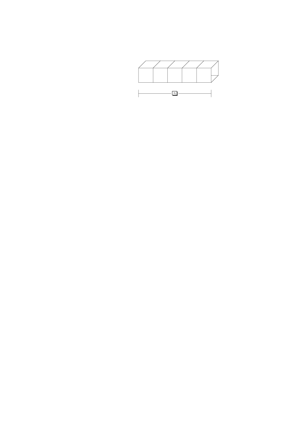
The graph contributing to the lowest order of the free energy density is a tube of length $N_{t}$ with a cross-section of one single plaquette. The contribution of these tubes together with inner plaquettes is

	$\displaystyle\mbox{SU(2):}\qquad f_{1}(N_{t},u)$	$\displaystyle=$	$\displaystyle-\frac{3}{N_{t}}u^{4N_{t}}a^{N_{t}},$		(6)
	$\displaystyle\mbox{SU(3):}\qquad f_{1}(N_{t},u)$	$\displaystyle=$	$\displaystyle-\frac{3}{N_{t}}u^{4N_{t}}\left[b^{N_{t}}+c^{N_{t}}\right],$		(7)

where $u$, $v$ and $w$ are the expansion parameters of the lowest dimensional representations of the corresponding gauge groups,

	$\displaystyle\mbox{SU(2):}\qquad u$	$\displaystyle=$	$\displaystyle\frac{\beta}{4}+{{\cal{O}}(\beta^{2})}\qquad v=\frac{\beta^{2}}{24}+{{\cal{O}}(\beta^{4})},\qquad$
	$\displaystyle\mbox{SU(3):}\qquad u$	$\displaystyle=$	$\displaystyle\frac{\beta}{18}+{{\cal{O}}(\beta^{2})}\qquad v=\frac{\beta^{2}}{432}+{{\cal{O}}(\beta^{4})}\qquad w=\frac{\beta^{2}}{288}+{{\cal{O}}(\beta^{4})},$		(8)

and we have used the abbreviations

	$\displaystyle a$	$\displaystyle=$	$\displaystyle 1+3v-4u^{2},$
	$\displaystyle b$	$\displaystyle=$	$\displaystyle 1-3u-6v+8w,$
	$\displaystyle c$	$\displaystyle=$	$\displaystyle 1+3u+6v+8w-18u^{2}.$		(9)

Higher order contributions consist of such tubes with local decorations of additional plaquettes either in the fundamental or in higher representations. For the interesting cases SU(2) and SU(3), these contributions up to the calculated orders are

	$\displaystyle\mbox{SU(2):}\quad f(N_{t},u)=$	$\displaystyle-$	$\displaystyle\frac{3}{N_{t}}u^{4N_{t}}a^{N_{t}}\left[1+12N_{t}u^{4}-\frac{1556}{81}N_{t}u^{6}+\left(86N_{t}^{2}+\frac{35828}{243}N_{t}\right)u^{8}\right],$		(10)
	$\displaystyle\mbox{SU(3):}\quad f(N_{t},u)=$	$\displaystyle-$	$\displaystyle\frac{3}{N_{t}}u^{4N_{t}}c^{N_{t}}\Big[1+12N_{t}u^{4}+42N_{t}u^{5}-\frac{115343}{2048}N_{t}u^{6}-\frac{1095327}{2048}N_{t}u^{7}\Big]$		(11)
		$\displaystyle-$	$\displaystyle\frac{3}{N_{t}}u^{4N_{t}}b^{N_{t}}\Big[1+12N_{t}u^{4}+30N_{t}u^{5}-\frac{17191}{256}N_{t}u^{6}+63N_{t}u^{7}\Big],$

which are valid only for $N_{t}\geq 5$. For smaller $N_{t}$ there are modifications of these formulae coming from polymers with cross-sections larger than one plaquette. The complete results for $N_{t}=2$ and $3$ in SU(2) are

	$\displaystyle N_{t}=2:\quad f(2,u)=$	$\displaystyle-$	$\displaystyle\frac{3}{2}u^{8}\left[1-4u^{2}+\frac{110}{3}u^{4}-\frac{58472}{405}u^{6}+\frac{64897681}{65610}u^{8}\right],$		(12)
	$\displaystyle N_{t}=3:\quad f(3,u)=$	$\displaystyle-$	$\displaystyle u^{12}\left[1-6u^{2}+50u^{4}-\frac{37966}{135}u^{6}+\frac{843898}{405}u^{8}\right],$		(13)

Recognizing the first orders of the corresponding glueball masses (see [2] and [3]) for SU(2)

	$\displaystyle m(A_{1}^{++})$	$\displaystyle=$	$\displaystyle-4\ln\,u+2u^{2}-\frac{98}{3}u^{4}-\frac{20984}{405}u^{6}-\frac{151496}{243}u^{8},$		(14)
	$\displaystyle m(E^{++})$	$\displaystyle=$	$\displaystyle-4\ln\,u+2u^{2}-\frac{26}{3}u^{4}+\frac{13036}{405}u^{6}-\frac{28052}{243}u^{8},$		(15)

and SU(3)

	$\displaystyle m(A_{1}^{++})$	$\displaystyle=$	$\displaystyle-4\ln\,u-3u+9u^{2}-\frac{27}{2}u^{3}-7u^{4}-\frac{297}{2}u^{5}+\frac{858827}{10240}u^{6}+\frac{47641149}{71680}u^{7},$		(16)
	$\displaystyle m(E^{++})$	$\displaystyle=$	$\displaystyle-4\ln\,u-3u+9u^{2}-\frac{27}{2}u^{3}+17u^{4}-\frac{153}{2}u^{5}+\frac{1104587}{10240}u^{6}+\frac{29577789}{71680}u^{7},$		(17)
	$\displaystyle m(T_{1}^{+-})$	$\displaystyle=$	$\displaystyle-4\ln\,u+3u+\frac{9}{2}u^{3}-\frac{98}{4}u^{4}+\frac{33}{4}u^{5}-\frac{36771}{1280}u^{6}+\frac{117897}{448}u^{7},$		(18)

one can write

	$\displaystyle SU(2):\qquad f(N_{t},u)$	$\displaystyle=$	$\displaystyle-\frac{1}{N_{t}}\left[e^{-m(A_{1}^{++})N_{t}}+2e^{-m(E^{++})N_{t}}+{\cal{O}}(u^{4})\right],$		(19)
	$\displaystyle SU(3):\qquad f(N_{t},u)$	$\displaystyle=$	$\displaystyle-\frac{1}{N_{t}}\left[e^{-m(A_{1}^{++})N_{t}}+2e^{-m(E^{++})N_{t}}+3e^{-m(T_{1}^{+-})N_{t}}+{\cal{O}}(u^{4})\right],$		(20)

corresponding to a gas of non-interacting glueballs in a hadron-resonance-gas model [4], where

$\displaystyle f\simeq-T\sum_{i}e^{-\frac{E_{i}}{T}}.$

(21)

This is a rather remarkable result. It allows to see from first principles that the pressure $p=-f$ is exponentially small in the confined phase, and it explains the success of the hadron-resonance-gas model in reproducing the confined phase equation of state. Since the partition function is not directly measurable in Monte-Carlo simulations, the pressure is usually obtained by the integral method [5], where the expectation values of derivatives are computed and then integrated numerically,

$\displaystyle\frac{p}{T^{4}}\,\bigg|_{\beta_{0}}^{\beta}=N_{t}^{4}\int_{\beta_{0}}^{\beta}d\beta^{\prime}\left[S_{0}-S_{T}\right],$

with $S_{0}=6P_{0}$ and $S_{T}=3(P_{t}+P_{s})$, where $P_{0}$ denotes the plaquette expectation value on symmetric lattices and $P_{t,s}$ are those of space-time and space-space plaquettes with $N_{t}<N_{s}$. The lower integration limit is usually set to zero by hand, arguing with an exponentially small pressure in the low temperature regime. Our results now justify this assumption from first principles.

Physical phase transitions limit the radius of convergence on the real $\beta$-axis, signalled by a singularity in the full free energy. We model the full function from the series coefficients by Padé approximants $[L,M]$ with

$\displaystyle[L,M](u)\equiv\frac{1+a_{1}u+\dots+a_{L}u^{L}}{b_{0}+b_{1}u+\dots+b_{M}u^{M}},$

and search for the zeroes of the denominator. The resulting $L+M=2,3,4$ Padé tables for $N_{t}=2,3$ with the nearest real singularities are shown in table (1).

Zeroes $u_{0}$ of the Padé approximant which are very close to a singularity often indicate that the singularity is superfluous and disappears as the full funtion is approached. Hence, removing the singularities with a nearby zero, we obtain estimates for the critical couplings, which are not far from the Monte Carlo results $\beta_{c}=1.8800(30)$ for $N_{t}=2$ and $\beta_{c}=2.1768(30)$ for $N_{t}=3$ [6].

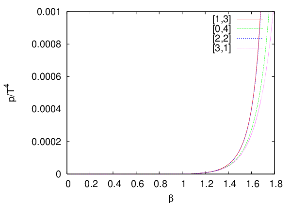
The $L+M=4$ Padé’s for $N_{t}=3$, SU(2), are shown in figure (2). The spread in the curves gives an estimate of the systematic error of the approximants at that order. The exponential suppression in the confined phase as well as the onset of the pressure upon approaching $T_{c}$ is reproduced by the strong coupling series.

Screening masses are defined by the exponential decay of the spatial correlation of suitable operators. We used plaquette operators in our calculations. Temporarily assigning separate gauge couplings to all plaquettes, the correlator can be defined as [2]

$$C(z)=\langle\mathrm{Tr}\,U_{p_{1}}(0)\,\,\mathrm{Tr}\,U_{p_{2}}(z)\rangle=N^{2}\frac{\partial^{2}}{\partial\beta_{1}\partial\beta_{2}}\ln\,Z(\beta,\beta_{1}\beta_{2})\bigg|_{\beta_{1,2}=\beta}.$$

(22)

At zero temperature the exponential decay is the same as for correlations in the time direction, and thus determined by the gluball masses, the lowest of which may be extracted as

$$m=-\lim_{z\rightarrow\infty}\frac{1}{z}\ln\,C(z).\\$$

(23)

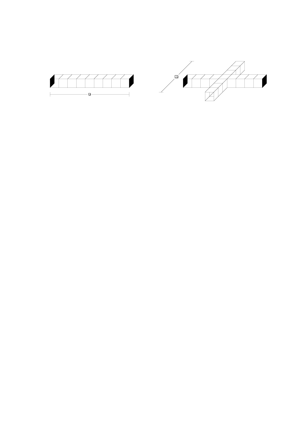
The leading order graphs for the strong coupling series are shown in figure (3). This leads to the lowest order contribution:

$$C(z)=A\,u^{4z}=A\mathrm{e}^{-m_{s}z}.$$

(24)

Thus the leading order for the screening mass is given by

$$m_{s}=-4\ln\,u(\beta).$$

(25)

The graph contributing to the lowest order of the difference between the screening masses at zero and finite temperature is shown in figure (3). To lowest order the mass difference is

	$\displaystyle\Delta m_{s}(N_{t})$	$\displaystyle=$	$\displaystyle m_{s}(N_{t})-m_{s}(\infty)$		(26)
		$\displaystyle=$	$\displaystyle-\frac{2}{3}N_{t}u^{4N_{t}-6}$		(28)

Thus one can see that the finite temperature effect on the screening mass is very small below $T_{c}$, as is also observed in Monte Carlo simulations (for references, see [7]).

References

- [1] I. Montvay and G. Münster, Quantum fields on a lattice, Cambridge University Press, UK (1994).
- [2] G. Münster, Strong Coupling Expansions For The Mass Gap In Lattice Gauge Theories, Nucl. Phys. B 190 (1981) 439.
- [3] K. Seo, Glueball Mass Estimate By Strong Coupling Expansion In Lattice Gauge Theories, Nucl. Phys. B 209 (1982) 200.
- [4] F. Karsch, K. Redlich and A. Tawfik, Thermodynamics at non-zero baryon number density: A comparison of lattice and hadron resonance gas model calculations, Phys. Lett. B 571 (2003) 67 [arXiv:hep-ph/0306208].
- [5] G. Boyd, J. Engels, F. Karsch, E. Laermann, C. Legeland, M. Lütgemeier and B. Petersson, Thermodynamics of SU(3) Lattice Gauge Theory, Nucl. Phys. B 469 (1996) 419 [arXiv:hep-lat/9602007].
- [6] J. Fingberg, F. Karsch and U. M. Heller, Scaling and asymptotic scaling in the SU(2) gauge theory, Nucl. Phys. Proc. Suppl. 30 (1993) 343 [arXiv:hep-lat/9208012].
- [7] E. Laermann and O. Philipsen, Status of lattice QCD at finite temperature, Ann. Rev. Nucl. Part. Sci. 53 (2003) 163 [arXiv:hep-ph/0303042].