跳到论文正文
W Papers独立论文阅读器 arXiv:0710.0491 论文正文 计算阅读时间 · 0%
引用这篇论文根据当前论文元数据生成,正式投稿前建议核对。


License: arXiv.org perpetual non-exclusive license
arXiv:0710.0491v2 [math.NA] 08 Jun 2011

Analysis of Linear Difference Schemes in the Sparse Grid Combination Technique

Christoph Reisinger Affiliation: Mathematical Institute, University of Oxford Affiliation: 24–29 St Giles, Oxford, OX1 3LB, United Kingdom Email: christoph.reisinger@maths.ox.ac.uk
Abstract

Sparse grids (Zenger 1990; Bungartz and Griebel 2004) are tailored to the approximation of smooth high-dimensional functions. On a dd-dimensional tensor product space, the number of grid points is N=𝒪⁡(h−1​|log⁡h|d−1)N=\mathcal{O}(h^{-1}|\log h|^{d-1}), where hh is a mesh parameter. The so-called combination technique, based on hierarchical decomposition and extrapolation, requires specific multivariate error expansions of the discretisation error on Cartesian grids to hold. We derive such error expansions for linear difference schemes through an error correction technique of semi-discretisations. We obtain overall error formulae of the type ε=𝒪⁡(hp​|log⁡h|d−1)\varepsilon=\mathcal{O}(h^{p}|\log h|^{d-1}) and analyse the convergence, with its dependence on dimension and smoothness, by examples of linear elliptic and parabolic problems, with numerical illustrations in up to eight dimensions.

Key words. Sparse grids, combination technique, error expansions, finite difference schemes

AMS subject classifications. 65N06, 65N12, 65N15, 65N40

1 Introduction

Models with high-dimensional state spaces play an important role in various applications. Important examples arise in financial engineering, more specifically in derivative pricing, which typically involve computation of expected pay-off functions with respect to a number of underlying stochastic factors, for instance share prices or interest rates. In the financial industry, this expectation is most commonly estimated by stochastic simulation, especially if the dimension exceeds three as is often the case. Recent computational studies suggest that sparse grid cubature (Gerstner et al. 2009), and the numerical solution of the corresponding Feynman-Kac PDE on sparse grids (Hilber et al. 2005; Reisinger and Wittum 2007; Leentvaar and Oosterlee 2008) are promising alternatives.

To give a further example of high-dimensional spaces, in quantum mechanics, high-dimensional eigenvalue problems for the Schrödinger equation govern the density functions associated with molecular systems. Again, recent analytical and numerical results (Garcke and Griebel 2000; Griebel and Hamaekers 2007; Yserentant 2010; Bachmayr 2010; Zeiser 2010) demonstrate the potential of sparse grids to make decisive progress in this area.

However, several of these works also give an account of the difficulties encountered, notably for problems with reduced regularity, but even for infinitely smooth solutions in higher dimensions. Although the asymptotic order of complexity of the sparse grid solution is only weakly dependent on the dimension, the “constants” in the error formulae reflect the dependence on both the dimension and on a measure of the variation of the solution. It is therefore an emphasis of this article to calculate all constants in painstaking detail.

Classical grid based methods in d>1d>1 dimensions suffer from the curse of dimensionality: the number of unknowns NN required to achieve a prescribed error ε\varepsilon grows exponentially in dd like

N(ε)=𝒪(ε−d/p),N(\varepsilon)=\mathcal{O}(\varepsilon^{-d/p}),

where pp is the order of the method.

The analysis in (Bungartz and Griebel 2004) shows that optimal approximation of sufficiently smooth functions, for a given size of a hierarchical tensor product basis, is attained for so-called sparse grids. Their relevance to the solution of PDEs was first revealed by Zenger 1990, and subsequently error bounds for finite element methods for elliptic problems were derived in detail by Bungartz 1992; Bungartz 1998. More recently, optimal convergence rates of a sparse wavelet method were obtained for parabolic equations, under weak assumptions on the regularity of the initial condition, using h​php discontinuous Galerkin time stepping in conjunction with the smoothing properties of parabolic equations (von Petersdorff and Schwab 2004). What is more, adaptive sparse wavelet methods retain this optimal order for elliptic equations in the presence of corner singularities of the solution (Nitsche 2005; Dijkema et al. 2009; Dauge and Stevenson 2010).

In contrast to Galerkin-type methods, the combination technique – first introduced in (Griebel et al. 1992) – decomposes the solution into contributions from tensor product grids. This facilitates the discretisation of PDEs has the practical advantage that only numerical approximations on relatively small conventional grids need to be computed. These can be obtained independently and are superposed subsequently, which lends itself to very efficient parallel implementations. This concept has been successfully used in a number of applications, e.g. computational fluid dynamics (Griebel and Thurner 1995), quantum mechanics (Garcke and Griebel 2000) and computational finance (Reisinger and Wittum 2007).

Theoretical results for this extrapolation scheme, however, which inevitably rely on the expansion of the hierarchical surplus in terms of the grid sizes, have so far only been obtained for simple model problems. Bungartz et al. 1994 obtain error bounds in terms of the Fourier coefficients for a central difference scheme for the two-dimensional Laplace equation. Pflaum 1997 and Pflaum and Zhou 1999 employ Sobolev space techniques for the combination solution of a finite element method and prove asymptotic errors of the form h2​|log⁡h|d−1h^{2}|\log h|^{d-1} in the L2L_{2}-norm for general linear elliptic equations in two dimensions, and first order convergence in the H1H^{1}-norm. A similar result is also shown for the Poisson equation in higher dimensions. Common to these two approaches is the use of semi-discrete solutions to derive expansions of the hierarchical surplus, namely Fourier representations for semi-discrete solutions to the Laplace problem in (Bungartz et al. 1994), and variational formulations with semi-discrete conforming subspaces in (Pflaum 1997; Pflaum and Zhou 1999).

We introduce a new framework to derive error bounds for general difference schemes in arbitrary dimensions. As in the aforementioned articles, again semi-discrete problems will play an important role, now in the somewhat different setting of an error correction scheme that determines a suitable error expansion by a simple generic recursion. This will be illustrated by the central difference stencil for the Poisson problem and with upwinding for the advection equation. For these two examples, sparse grid error bounds are then derived in terms of the dimension of the problem and the smoothness of the solution. The results are formulated in spaces in which mixed derivatives of sufficiently high order exist and vanish at the boundaries, in order to avoid regularity problems in the corners. We will discuss in the following section why this is not a problematic assumption for most practical applications where one would use sparse grids.

The rest of the paper is organised as follows. Section 2 outlines the workings of the sparse grid combination technique, the two main steps of the convergence analysis, and discusses smoothness requirements. Section 3 develops a framework for the first problem-specific step of the analysis, in which we derive a multivariate expansion of the form (6) for the error u⁡(𝐱h)−𝐮hu({\bf x}_{h})-{\bf u}_{h} between the numerical solution 𝐮h{\bf u}_{h} and exact solution uu at the grid points 𝐱h{\bf x}_{h}. We derive exact coefficients for the Poisson problem and some extensions to illustrate the application of the framework. We then extend the grid solution to [0,1]d[0,1]^{d} by multilinear interpolation in Section 4, and show that the expansion (6) is maintained pointwise for the error between the exact solution uu and the interpolated approximation ℐ​𝐮h\mathcal{I}{\bf u}_{h}. In the second step of the analysis, in Section 5, these error expansions on Cartesian grids are used to estimate the error of the combined solution by combinatorial formulae. Exact asymptotic expansions will be given. In Section 6, numerical results for carefully chosen model problems are discussed to illustrate the theory. In particular, we highlight the dependence of the error on the smoothness of the solution and the problem dimension. Section 7 discusses these results and points out future directions, extensions to other problem classes and possible applications.

2 The combination technique and main results

Consider the dd-dimensional unit cube Id=[0,1]dI^{d}=[0,1]^{d} and a Cartesian grid with mesh sizes hi=2−lih_{i}=2^{-l_{i}}, corresponding to a level li∈ℕ0l_{i}\in\mathbb{N}_{0} in direction i=1,…,di=1,\ldots,d.

For a vector 𝐡=(hi)1≤i≤d{\bf h}=(h_{i})_{1\leq i\leq d} we denote by u𝐡u_{{\bf h}} the approximation of a function on this grid with points 𝐱h=(ij​hj)0≤ij≤Nj,1≤j≤d{\bf x}_{h}=(i_{j}h_{j})_{\scriptsize\begin{array}[]{l}0\leq i_{j}\leq N_{j},1\leq j\leq d\end{array}}\!\!, Nj=1/hj=2ljN_{j}=1/h_{j}=2^{l_{j}}. Hereby 𝐮h{\bf u}_{h} is the discrete vector of (approximated) values at the grid points, which is extended to IdI^{d} by a suitable interpolation operator ℐ\mathcal{I} as u𝐡:=ℐ​𝐮hu_{{\bf h}}:=\mathcal{I}{\bf u}_{h}. We will ultimately be concerned with a setting where 𝐮h{\bf u}_{h} is the finite difference solution to a scalar PDE, in which case 𝐮h{\bf u}_{h} is different from the vector obtained by evaluating the exact solution to the PDE, uu, at the grid points. Therefore we denote the latter by u⁡(𝐱h)u({\bf x}_{h}).

Figure 1: Full grid ℳ¯4\overline{\mathcal{M}}_{4}, sparse grid ℳ4\mathcal{M}_{4}, and a possible realisation of a dimension adaptive sparse grid ℳ¯4\underline{\mathcal{M}}_{4}.

We now define the family UU of solutions corresponding to these grids (see Fig. 1) by U=(U⁡(𝐢))𝐢∈ℕ0dU=(U({\bf i}))_{{\bf i}\in\mathbb{N}_{0}^{d}} with

U⁡(𝐢):=u2−𝐢,U({\bf i}):=u_{2^{-{\bf i}}},

i.e. as the family of numerical approximations u𝐡u_{{\bf h}} on tensor product grids with hk=2−ikh_{k}=2^{-i_{k}}. Then the hierarchical surplus is the sequence

δ​U:=δ1​…​δd​U,\delta U:=\delta_{1}\ldots\delta_{d}U, (1)

where

δk​U​(𝐢):={U⁡(𝐢)−U⁡(𝐢−𝐞k)ik>0,U⁡(𝐢)ik=0,\displaystyle\delta_{k}U({\bf i}):=\left\{\begin{array}[]{rl}U({\bf i})-U({\bf i}-{\bf e}_{k})&i_{k}>0,\\ U({\bf i})&i_{k}=0,\end{array}\right.

and 𝐞k{\bf e}_{k} the kk-th unit vector. The difference operators commute.

Given a sequence of index sets ℳn⊂ℕ0d\mathcal{M}_{n}\subset\mathbb{N}_{0}^{d}, the approximation on level nn is now defined as

un:=∑𝐢∈ℳnδ​U​(𝐢).u_{n}:=\sum_{{\bf i}\in\mathcal{M}_{n}}\delta U({\bf i}). (5)

If this series converges in absolute terms, the error

‖un−u‖=‖∑𝐢∉ℳnδ​U​(𝐢)‖≤∑𝐢∉ℳn‖δ​U​(𝐢)‖\|u_{n}-u\|=\Big\|\sum_{{\bf i}\notin\mathcal{M}_{n}}\delta U({\bf i})\Big\|\leq\sum_{{\bf i}\notin\mathcal{M}_{n}}\|\delta U({\bf i})\|

in a suitable norm ∥⋅∥\|\cdot\| is therefore bounded by the surplus on finer grids which are not considered in the approximation at level nn. The choice of an optimal refinement strategy is thus determined by control of the surplus. If this is done a posteriori, dimension adaptive schemes are obtained (Hegland 2003; Gerstner and Griebel 2003; Griebel and Holtz 2010). This requires that hierarchical surpluses on finer levels are estimated from coarser levels. Conversely, an a priori analysis requires analytic estimates of the surplus in terms of the grid sizes h1,…,hdh_{1},\ldots,h_{d} and is the focus of this paper.

Griebel et al. 1992 propose a splitting into lower-dimensional contributions of the form

u−u𝐡=∑m=1d∑{j1,…,jm}⊂{1,…,d}γj1,…,jm​(⋅,hj1,…,hjm)​hj1p⋅…⋅hjmpu-u_{{\bf h}}=\sum_{m=1}^{d}\sum_{\tiny\begin{array}[]{c}\{j_{1},\ldots,j_{m}\}\\ \subset\{1,\ldots,d\}\end{array}}\gamma_{j_{1},\ldots,j_{m}}(\cdot;h_{j_{1}},\ldots,h_{j_{m}})h_{j_{1}}^{p}\cdot\ldots\cdot h_{j_{m}}^{p} (6)

to analyse the combination technique. The ‘⋅\cdot’ stands for the arguments of uu. Before we turn to the derivation of such expansions, we briefly outline the importance for the combination technique.

If we view the continuous function uu as a constant sequence over all refinement levels, and therefore set δ​u=0\delta u=0, then under assumption (6)

δ​U​(𝐢)=δ⁡(U⁡(𝐢)−u)=𝒪⁡(2−p​|𝐢|),\delta U({\bf i})=\delta\left(U({\bf i})-u\right)=\mathcal{O}\left(2^{-p|{\bf i}|}\right), (7)

where |𝐢|=|𝐢|1:=∑k=1dik|{\bf i}|=|{\bf i}|_{1}:=\sum_{k=1}^{d}i_{k} and all lower order terms cancel out through the difference operator. Thus an asymptotically optimal choice for the index set for (5) is

ℳn={𝐢∈ℕ0d:|𝐢|≤n}.\mathcal{M}_{n}=\{{\bf i}\in\mathbb{N}_{0}^{d}:|{\bf i}|\leq n\}.

The number of elements of ℳn\mathcal{M}_{n} is then obtained by

|ℳn/ℳn−1|=(n+d−1d−1)⇒|ℳn|=∑l=0n(l+d−1d−1)=𝒪⁡(nd−1),|\mathcal{M}_{n}/\mathcal{M}_{n-1}|=\left(\begin{array}[]{c}n+d-1\\ d-1\end{array}\right)\quad\Rightarrow\quad|\mathcal{M}_{n}|=\sum_{l=0}^{n}\left(\begin{array}[]{c}l+d-1\\ d-1\end{array}\right)=\mathcal{O}(n^{d-1}),

and the number of nodes in the grid corresponding to an index 𝐢{\bf i} is bounded by ∏k=1d(2ik+1)=𝒪⁡(2|𝐢|)\prod_{k=1}^{d}(2^{i_{k}}+1)=\mathcal{O}\left(2^{|{\bf i}|}\right). For this choice of grid we conclude from (7) that

‖u−un‖≤∑𝐢∉ℳn‖δ​U​(𝐢)‖≤∑|𝐢|>n𝒪⁡(2−p​|𝐢|)=𝒪⁡(nd−1​2−p​n).\displaystyle\|u-u_{n}\|\leq\sum_{{\bf i}\notin\mathcal{M}_{n}}\|\delta U({\bf i})\|\leq\sum_{|{\bf i}|>n}\mathcal{O}(2^{-p|{\bf i}|})=\mathcal{O}(n^{d-1}2^{-pn}). (8)

The significance of the result (8) is that although the number of degrees of freedom is only

Nd​o​f=𝒪⁡(nd−1​2n),N_{dof}=\mathcal{O}\left(n^{d-1}2^{n}\right),

compared to 2d​n2^{dn} on the full grid, the error only deteriorates by a factor of order nd−1n^{d-1} compared to the full grid result 2−p​n2^{-pn}.

We illustrate the combination formula by a two-dimensional example:

u0\displaystyle u_{0} =\displaystyle= u⁡(0,0)\displaystyle u(0,0)
u1\displaystyle u_{1} =\displaystyle= [u⁡(1,0)−u⁡(0,0)]+[u⁡(0,1)−u⁡(0,0)]+u0\displaystyle[u(1,0)-u(0,0)]+[u(0,1)-u(0,0)]+u_{0}
=\displaystyle= [u⁡(1,0)+u⁡(0,1)]−u⁡(0,0)\displaystyle[u(1,0)+u(0,1)]-u(0,0)
u2\displaystyle u_{2} =\displaystyle= [u⁡(2,0)−u⁡(1,0)]+[u⁡(1,1)−u⁡(1,0)−u⁡(0,1)+u⁡(0,0)]+[u⁡(0,2)−u⁡(0,1)]+u1\displaystyle[u(2,0)-u(1,0)]+[u(1,1)-u(1,0)-u(0,1)+u(0,0)]+[u(0,2)-u(0,1)]+u_{1}
=\displaystyle= [u⁡(2,0)+u⁡(1,1)+u⁡(0,2)]−[u⁡(1,0)+u⁡(0,1)].\displaystyle[u(2,0)+u(1,1)+u(0,2)]-[u(1,0)+u(0,1)].

The general structure in two dimensions is

un=∑l=0nU⁡(l,n−l)−∑l=0n−1U⁡(l,n−1−l).u_{n}=\sum_{l=0}^{n}U(l,n-l)-\sum_{l=0}^{n-1}U(l,n-1-l).

In one dimension, the sparse grid is identical to the full grid. In general, for d≥1d\geq 1 and n>d−1n>d-1, the combined solution can be written as

un\displaystyle u_{n} =\displaystyle= [δ1d−1​S]​(n),\displaystyle[\delta_{1}^{d-1}S](n),
S⁡(n)\displaystyle S(n) =\displaystyle= ∑|𝐢|=nU⁡(𝐢),\displaystyle\sum_{|{\bf i}|=n}U({\bf i}),

where the difference operator δ1\delta_{1}, applied d−1d-1 times to the index nn of SS, is the one-dimensional version of (1), (2). Evaluating the coefficients explicitly gives

un=∑l=n−d+1nan−l​S​(n),u_{n}=\sum_{l=n-d+1}^{n}\!\!\!a_{n-l}\;S(n), (9)

where

ai:=(−1)d−1−i​(d−1i),0≤i≤d−1.a_{i}:=(-1)^{d-1-i}\left(\begin{array}[]{c}d-1\\ i\end{array}\right),\quad 0\leq i\leq d-1. (10)

The error analysis falls into two main parts: If an expansion (6) can be shown for the problem at hand, then error bounds of the form (8) follow by combinatorial arguments.

For the first problem-dependent part, we consider here linear PDEs on Id=[0,1]dI^{d}=[0,1]^{d} and denote by ∂iu\partial_{i}u the partial derivative of uu with respect to xix_{i}. For a multi-index 𝜶=(α1,…,αd)\boldsymbol{\alpha}=(\alpha_{1},\ldots,\alpha_{d}), let D𝜶​u=∂1α1…​∂dαduD^{\boldsymbol{\alpha}}u=\partial_{1}^{\alpha_{1}}\ldots\partial_{d}^{\alpha_{d}}u. It will become clear later that the appropriate function spaces are those with bounded mixed derivatives in the supremum norm ∥⋅∥∞\|\cdot\|_{\infty},

X𝜶d\displaystyle X_{\boldsymbol{\alpha}}^{d} :⁣=\displaystyle:= {u:[0,1]d→ℝ:D𝜷u∈C0(Id)∀𝜷≤𝜶}\displaystyle\left\{u:[0,1]^{d}\rightarrow\mathbb{R}:\;D^{\boldsymbol{\beta}}u\in C_{0}(I^{d})\;\forall\boldsymbol{\beta}\leq\boldsymbol{\alpha}\right\} (11)
X𝜶d​(K)\displaystyle X_{\boldsymbol{\alpha}}^{d}(K) :⁣=\displaystyle:= {u∈X𝜶d:‖D𝜷​u‖∞≤K​∀𝜷≤𝜶}\displaystyle\left\{u\in X_{\boldsymbol{\alpha}}^{d}:\;\|D^{\boldsymbol{\beta}}u\|_{\infty}\leq K\;\forall\boldsymbol{\beta}\leq\boldsymbol{\alpha}\right\} (12)
Xkd\displaystyle X_{k}^{d} :⁣=\displaystyle:= {u:[0,1]d→ℝ:D𝜶u∈C0(Id)∀𝜶∈{0,…,k}d}\displaystyle\left\{u:[0,1]^{d}\rightarrow\mathbb{R}:\;D^{\boldsymbol{\alpha}}u\in C_{0}(I^{d})\;\forall\boldsymbol{\alpha}\in\{0,\ldots,k\}^{d}\right\} (13)
Xkd​(K)\displaystyle X_{k}^{d}(K) :⁣=\displaystyle:= {u∈Xkd:‖D𝜶​u‖∞≤K​∀𝜶∈{0,…,k}d}.\displaystyle\left\{u\in X_{k}^{d}:\;\|D^{\boldsymbol{\alpha}}u\|_{\infty}\leq K\;\forall\boldsymbol{\alpha}\in\{0,\ldots,k\}^{d}\right\}. (14)

By C0​(Id)C_{0}(I^{d}) we denote the space of continuous functions which are zero at the boundary, so we require for Xkd​(K)X_{k}^{d}(K) that all mixed derivatives up to order kk vanish at the boundary. We will now discuss the smoothness requirements, and anticipate the following detailed results from the analysis in Section 5.

Theorem 2.1.

Let u∈X4du\in X_{4}^{d} be a solution of the Poisson problem and unu_{n} the sparse grid solution with central differences on level nn. Then

‖u−un‖∞≤c⋅sup|𝜶|∞≤4‖D𝜶​u‖∞⋅d⋅(52)d⋅(n+2​(d−1))d−1⋅4−n,\|u-u_{n}\|_{\infty}\leq c\cdot\sup_{|\boldsymbol{\alpha}|_{\infty}\leq 4}\|D^{\boldsymbol{\alpha}}u\|_{\infty}\cdot d\cdot\left(\frac{5}{2}\right)^{d}\cdot(n+2(d-1))^{d-1}\cdot 4^{-n}, (15)

where c≤121000c\leq 121000, 𝛂=(4,…,4)\boldsymbol{\alpha}=(4,\ldots,4), and

u−un=c~⋅d43​d⋅nd−1⋅4−n+𝒪⁡(nd−2​4−n),u-u_{n}=\tilde{c}\cdot\frac{d}{4^{3d}}\cdot n^{d-1}\cdot 4^{-n}+\mathcal{O}\left(n^{d-2}4^{-n}\right), (16)

for some c~≤c​‖D𝛂​u‖∞\tilde{c}\leq c\|D^{\boldsymbol{\alpha}}u\|_{\infty}.

Theorem 2.2.

Let u∈X2du\in X_{2}^{d} be a solution of the advection equation and unu_{n} the sparse grid solution with upwinding and backward Euler timestepping on level nn. Then

‖u−un‖∞≤c⋅sup|𝜶|∞≤2‖D𝜶​u‖∞⋅d⋅(34)d⋅(n+2​(d−1))d−1⋅2−n,\|u-u_{n}\|_{\infty}\leq c\cdot\sup_{|\boldsymbol{\alpha}|_{\infty}\leq 2}\|D^{\boldsymbol{\alpha}}u\|_{\infty}\cdot d\cdot\left(\frac{3}{4}\right)^{d}\cdot(n+2(d-1))^{d-1}\cdot 2^{-n}, (17)

where c≤2c\leq 2, 𝛂=(2,…,2)\boldsymbol{\alpha}=(2,\ldots,2), and

u−un=c~⋅d4d⋅nd−1⋅2−n+𝒪⁡(nd−2​2−n),u-u_{n}=\tilde{c}\cdot\frac{d}{4^{d}}\cdot n^{d-1}\cdot 2^{-n}+\mathcal{O}\left(n^{d-2}2^{-n}\right), (18)

for some c~≤c​‖D𝛂​u‖∞\tilde{c}\leq c\|D^{\boldsymbol{\alpha}}u\|_{\infty}.

The above theorems give error bounds of order |log⁡h|d−1​hp|\log h|^{d-1}h^{p}, and moreover make the asymptotic dependence of constants on the dimensionality and smoothness explicit. The analysis will show how these results generalise to a wider class of linear elliptic and parabolic PDEs, although an explicit computation of the constants is omitted in the general case.

Equations (16) and (18) shows that for fixed nn, the coefficients of nd−1​2−p​nn^{d-1}2^{-pn} go to 00 as d→∞d\rightarrow\infty, in line with observations in (Griebel 2006) and (Schwab et al. 2008). This does not mean, however, that the approximation for a given level is better in higher dimensions, due to the presence of the polynomial term in nn. Moreover, this asymptotic approximation is obtained under the assumption that nn is large compared to dd, and this asymptotic range is reached for increasing nn in higher dimensions, as will be confirmed in the numerical results later. This behaviour is also related to the fact that the minimum number of levels contained in the combination solution grows linearly in dd.

In the special case c~=0\tilde{c}=0, the leading term proportional to nd−1​2−p​nn^{d-1}2^{-pn} vanishes. This is the case if the solution has a low superposition dimension, i.e. is a sum of functions that depend only on a subset of the coordinates. In applications, this is often approximately the case, as can be seen by asymptotic expansion (Reisinger and Wittum 2007). This effect can be exploited to construct generalised sparse grids to reduce the complexity to that of lower-dimensional sparse grids.

We now return to the question of smoothness of solutions, a key prerequisite for sparse grid approximation. Due to the corners of the domain, the solution usually does not inherit the necessary degree of smoothness from the data, e.g. for the Poisson problem, with homogeneous Dirichlet data on the dd-cube, the solution for right hand-side f=1f=1 does not have uniformly bounded mixed derivatives. Rather, certain compatibility conditions for ff need to be satisfied. For completeness, conditions for sufficient regularity are derived in Appendix A.1, and estimates for the derivatives of solutions are given in Appendix A.2. This may seem to restrict the applicability of these results, and of sparse grids more generally, to a small class of problems of limited practical value. We will now explain why this is not the case.

In most practically relevant high-dimensional applications, we are not interested in boundary value problems on the unit cube as such, but in equations on ℝd\mathbb{R}^{d}. The localisation is necessary to make the problem computable on a grid, while a box shape of the computational domain is amenable to tensor product grids. Boundary values are typically chosen by asymptotic analysis of the unbounded problem to ensure that by making the box BB large enough, the difference between the original solution and the localised one can be made small. Now the unbounded solution restricted to the box is smooth, and therefore the exact solution to the BVP with asymptotic boundary data, albeit usually not smooth itself, is a small perturbation of a smooth function. Therefore, if the asymptotic boundary conditions are accurate to some ϵ\epsilon, and the discretisation on each subgrid of the sparse grid is stable with respect to the boundary data, which is normally given, then the combined sparse grid error due to the boundary approximation is of order ϵ​|log⁡h|d−1\epsilon|\log h|^{d-1}, where |log⁡h|d−1|\log h|^{d-1} is the number of subgrids involved. The error of the hypothetical discretisation of a BVP with exact boundary data on the cube is of order Lq​hp​|log⁡h|d−1L^{q}h^{p}|\log h|^{d-1}, as the continuous solution to this problem is smooth. The factor LqL^{q}, for some qq and with LL the size of the box, arises because of the transformation of the solution and its derivatives to the unit cube. The sum of the localisation and discretisation errors is a bound for the discretisation error of the non-smooth localised solution. Indeed, we want to approximate the unbounded solution, but we have assumed that the localisation error is bounded by ϵ\epsilon. In many applications, asymptotic boundary values are known which converge exponentially to the true solution, as is seen e.g. for multi-dimensional Black-Scholes-type PDEs from (Kangro and Nicolaides 2001). In these cases, one can therefore first pick the domain BB large enough and then hh to achieve a desired overall accuracy, without affecting the complexity order.

This justifies restricting the following error analysis to the setting where smooth solutions exist, in particular we consider solutions which vanish sufficiently fast at the boundaries.

3 Error expansion for finite difference schemes

The goal of this section is to establish error expansions of the form

u⁡(𝐱h)−𝐮h=∑m=1d∑{j1,…,jm}⊂{1,…,d}wj1,…,jm​(𝐱h,hj1,…,hjm)​hj1p⋅…⋅hjmp,u({\bf x}_{h})-{\bf u}_{h}=\sum_{m=1}^{d}\sum_{\tiny\begin{array}[]{c}\{j_{1},\ldots,j_{m}\}\\ \subset\{1,\ldots,d\}\end{array}}w_{j_{1},\ldots,j_{m}}({\bf x}_{h};h_{j_{1}},\ldots,h_{j_{m}})h_{j_{1}}^{p}\cdot\ldots\cdot h_{j_{m}}^{p}, (19)

between the finite difference solution 𝐮h{\bf u}_{h} and the exact solution uu of a PDE, evaluated on a Cartesian grid 𝐱h{\bf x}_{h} with grid sizes h1,…,hdh_{1},\ldots,h_{d}.

We have in mind linear (possibly degenerate) elliptic equations of the type

A​u=∑i,j=1dai​j​∂i∂ju+∑j=1dbj​∂ju+c​u=f,Au=\sum_{i,j=1}^{d}a_{ij}\partial_{i}\partial_{j}u+\sum_{j=1}^{d}b_{j}\partial_{j}u+cu=f,

where ∑i,j=1dni​nj​ai​j≥0\sum_{i,j=1}^{d}n_{i}n_{j}a_{ij}\geq 0, and view parabolic equations as a degenerate case.

3.1 Setup

It seems instructive to first outline the main principles of the proof, which are generic and can be applied to a large class of problems. We write the discretised systems in matrix notation

𝐀h​𝐮h=𝐟h,{\bf A}_{h}{\bf u}_{h}={\bf f}_{h}, (20)

such that the truncation error can be written as 𝐀h​u​(𝐱h)−𝐟h{\bf A}_{h}u({\bf x}_{h})-{\bf f}_{h}.

In order to split up the truncation error into contributions from different dimensions, we define semi-discrete operators 𝐀h(i1,…,im){\bf A}^{(i_{1},\ldots,i_{m})}_{h} in directions i1,…,imi_{1},\ldots,i_{m}, e.g. for the Laplace operator,

𝐀h(i1,…,im)​u=∑i∈{i1,…,im}δi,hi+​δi,hi−​u+∑i∉{i1,…,im}∂i2u,{\bf A}^{(i_{1},\ldots,i_{m})}_{h}u=\sum_{i\in\{i_{1},\ldots,i_{m}\}}\delta^{+}_{i,h_{i}}\delta^{-}_{i,h_{i}}u+\sum_{i\notin\{i_{1},\ldots,i_{m}\}}\partial_{i}^{2}u, (21)

where δk,hk+\delta_{k,h_{k}}^{+} and δk,hk−\delta_{k,h_{k}}^{-} are one-sided differences such that δi,hi+​δi,hi−\delta^{+}_{i,h_{i}}\delta^{-}_{i,h_{i}} is a second difference.

In contrast to the fully discrete solutions 𝐮h{\bf u}_{h} satisfying (20), this leads to a system of PDEs

𝐀h(i1,…,im)​𝐮h(i1,…,im)=𝐟h(i1,…,im),{\bf A}^{(i_{1},\ldots,i_{m})}_{h}{\bf u}^{(i_{1},\ldots,i_{m})}_{h}={\bf f}^{(i_{1},\ldots,i_{m})}_{h},

with boundary conditions, where 𝐮h(i1,…,im){\bf u}^{(i_{1},\ldots,i_{m})}_{h} are defined on hyper-planes

𝐈(i1,…,im)={x∈Id:xik∈{jhik: 0≤j≤hik−1},1≤k≤m},{\bf I}^{(i_{1},\ldots,i_{m})}=\{x\in I^{d}:\;x_{i_{k}}\in\{jh_{i_{k}}:\;0\leq j\leq h_{i_{k}}^{-1}\},1\leq k\leq m\},

and 𝐟h(i1,…,im)=𝐑h(i1,…,im)​f{\bf f}^{(i_{1},\ldots,i_{m})}_{h}={\bf R}^{(i_{1},\ldots,i_{m})}_{h}f is the restriction of ff to 𝐈(i1,…,im){\bf I}^{(i_{1},\ldots,i_{m})}. Let C⁡(𝐈(i1,…,im))C({\bf I}^{(i_{1},\ldots,i_{m})}) denote the space of continuous functions on these planes with maximum norm ∥⋅∥∞\|\cdot\|_{\infty}, and derivatives are defined in directions along the planes.

We restrict the following sketch of the proof to two space dimensions in order to avoid cumbersome notation. We then extend this to higher dimensions and specify the requirements for particular examples, derive the coefficients in the expansion (19) and give sharp bounds.

3.2 Outline of proof in two dimensions

Starting point is a consistency assumption of order pp of the form

𝐀h​u−f=h1p​τ1(0)​(⋅,h1)+h2p​τ2(0)​(⋅,h2)+h1p​h2p​τ1,2(0)​(⋅,h1,h2).\displaystyle{\bf A}_{h}u-f=h_{1}^{p}\tau_{1}^{(0)}(\cdot,h_{1})+h_{2}^{p}\tau_{2}^{(0)}(\cdot,h_{2})+h_{1}^{p}h_{2}^{p}\tau_{1,2}^{(0)}(\cdot,h_{1},h_{2}). (22)

This will typically be straightforward to obtain by Taylor expansion. In so doing, we assume that the solution is sufficiently smooth, and we make such an assumption throughout the following considerations. Note that often, e.g. for the Poisson problem, τ1,2(0)​(⋅,h1,h2)=0\tau_{1,2}^{(0)}(\cdot,h_{1},h_{2})=0, but this term will be present, e.g., for the discretisation of mixed derivatives.

To derive the respective convergence order, one would be tempted to write

u⁡(𝐱h)−𝐀h−1​𝐟h⏟𝐮h=h1p​𝐀h−1​τ1(0)​(𝐱h,h1)+h2p​𝐀h−1​τ2(0)​(𝐱h,h2)+h1p​h2p​𝐀h−1​τ1,2(0)​(𝐱h,h1,h2),\displaystyle u({\bf x}_{h})\!-\!\underbrace{{\bf A}_{h}^{-1}{\bf f}_{h}}_{{\bf u}_{h}}=h_{1}^{p}{\bf A}_{h}^{-1}\tau_{1}^{(0)}({\bf x}_{h},h_{1})+h_{2}^{p}{\bf A}_{h}^{-1}\tau_{2}^{(0)}({\bf x}_{h},h_{2})+h_{1}^{p}h_{2}^{p}{\bf A}_{h}^{-1}\tau_{1,2}^{(0)}({\bf x}_{h},h_{1},h_{2}), (23)

and deduce from the boundedness of 𝐀h−1{\bf A}_{h}^{-1} convergence of the scheme. In the present context, however, since 𝐀h−1{\bf A}_{h}^{-1} depends on all grid sizes h1,…,hdh_{1},\ldots,h_{d}, it is not possible to derive an error expansion of the form (19) in this way, unless 𝐀h−1{\bf A}_{h}^{-1} is known explicitly in terms of the grid sizes and an expansion of 𝐀h−1{\bf A}_{h}^{-1} can be derived. This is the principle behind the seminal work of Bungartz et al. 1994, where Fourier series of continuous and discrete solutions to the Laplace equation are used. Note that this is only possible in special cases where such representations are known.

This is where the concept of error correction comes into play. We determine the error terms by solving the auxiliary semi-discrete problems

𝐀h(1)​w1​(⋅,h1)\displaystyle{\bf A}_{h}^{(1)}w_{1}(\cdot,h_{1}) =\displaystyle= τ1(0)​(⋅,h1)\displaystyle\tau^{(0)}_{1}(\cdot;h_{1}) (24)
𝐀h(2)​w2​(⋅,h2)\displaystyle{\bf A}_{h}^{(2)}w_{2}(\cdot,h_{2}) =\displaystyle= τ2(0)​(⋅,h2)\displaystyle\tau^{(0)}_{2}(\cdot;h_{2}) (25)

on the stacks of lines 𝐈h(1){{\bf I}}_{h}^{(1)} and 𝐈h(2){{\bf I}}_{h}^{(2)}, respectively. The crucial point is that w1​(⋅,h1)w_{1}(\cdot,h_{1}) and w2​(⋅,h2)w_{2}(\cdot,h_{2}) indeed only depend on h1h_{1} and h2h_{2} respectively, because they are the solution of a semi-discretisation as in (21) and not of the fully discrete equation.

Under suitable regularity assumptions, the first terms on the right-hand side of

𝐀h​(u−h1p​w1​(⋅,h1)−h2p​w2​(⋅,h2))−f\displaystyle{\bf A}_{h}\left(u-h_{1}^{p}w_{1}(\cdot;h_{1})-h_{2}^{p}w_{2}(\cdot;h_{2})\right)-f =\displaystyle=
h1p​(𝐀h(1)​w1​(⋅,h1)−𝐀h​w1​(⋅,h1))+h2p​(𝐀h(2)​w2​(⋅,h2)−𝐀h​w2​(⋅,h2))+h1p​h2p​τ12(0)​(⋅,h1,h2)\displaystyle\hskip-190.63338pth_{1}^{p}\left({\bf A}_{h}^{(1)}w_{1}(\cdot;h_{1})-{\bf A}_{h}w_{1}(\cdot;h_{1})\right)+h_{2}^{p}\left({\bf A}_{h}^{(2)}w_{2}(\cdot;h_{2})-{\bf A}_{h}w_{2}(\cdot;h_{2})\right)+h_{1}^{p}h_{2}^{p}\tau_{12}^{(0)}(\cdot;h_{1},h_{2})

can be absorbed in the higher order terms by further expanding

[𝐀h(1)−𝐀h]​w1​(⋅,h1)\displaystyle\left[{\bf A}_{h}^{(1)}-{\bf A}_{h}\right]w_{1}(\cdot;h_{1}) =\displaystyle= h2p​σ1;2​(⋅,h1,h2),\displaystyle h_{2}^{p}\,\sigma_{1;2}(\cdot;h_{1};h_{2}), (26)
[𝐀h(2)−𝐀h]​w2​(⋅,h2)\displaystyle\left[{\bf A}_{h}^{(2)}-{\bf A}_{h}\right]w_{2}(\cdot;h_{2}) =\displaystyle= h1p​σ2;1​(⋅,h2,h1),\displaystyle h_{1}^{p}\,\sigma_{2;1}(\cdot;h_{2};h_{1}), (27)

using the truncation error of the semi-discrete problems. So if we define

τ1,2(1)=τ1,2(0)+σ1;2​(⋅,h1,h2)+σ2;1​(⋅,h2,h1),\tau^{(1)}_{1,2}=\tau^{(0)}_{1,2}+\sigma_{1;2}(\cdot;h_{1};h_{2})+\sigma_{2;1}(\cdot;h_{2};h_{1}),

we get

𝐀h​(u−h1p​w1​(⋅,h1)−h2p​w2​(⋅,h2))−f=h1p​h2p​τ1,2(1)​(⋅,h1,h2).\displaystyle{\bf A}_{h}\left(u-h_{1}^{p}\,w_{1}(\cdot;h_{1})-h_{2}^{p}\,w_{2}(\cdot;h_{2})\right)-f=h_{1}^{p}h_{2}^{p}\,\tau^{(1)}_{1,2}(\cdot;h_{1},h_{2}).

Now we can conclude with a final step as in (23) that

u⁡(𝐱h)−𝐮h=h1p​w1​(𝐱h,h1)+h2p​w2​(𝐱h,h2)+h1p​h2p​w1,2​(𝐱h,h1,h2),\displaystyle u({\bf x}_{h})-{\bf u}_{h}=h_{1}^{p}\,w_{1}({\bf x}_{h};h_{1})+h_{2}^{p}\,w_{2}({\bf x}_{h};h_{2})+h_{1}^{p}h_{2}^{p}\,w_{1,2}({\bf x}_{h};h_{1},h_{2}), (28)

where

w1,2​(𝐱h,h1,h2)=𝐀h−1​τ1,2(1)​(𝐱h,h1,h2).w_{1,2}({\bf x}_{h};h_{1},h_{2})={\bf A}_{h}^{-1}\tau^{(1)}_{1,2}({\bf x}_{h};h_{1},h_{2}).

In higher dimensions, this procedure will be applied inductively. The start of the induction, m=1m=1, is always the consistency assumption (22). The final step, m=d+1m=d+1, is always essentially equivalent to (28).

The central proofs in this article go along these lines and it will become clear how this framework can be applied to other settings. The main gap in the above formal derivation concerns the existence of an expansion (26), (27), and the boundedness of its coefficients, which relies on the smoothness of the solutions of (24), (25). In the following two sections we detail the regularity requirements and give explicit bounds on the coefficients in the expansion for the Poisson problem and the advection equation.

3.3 Detailed analysis for the Poisson problem

As an example, we consider central differences for the Poisson problem

Δ​u=∑i=1d∂i2u=f\displaystyle\Delta u=\sum_{i=1}^{d}\partial_{i}^{2}u=f in ​Id,\displaystyle\text{in }I^{d}, (29)
u=0\displaystyle u=0 on ​∂Id,\displaystyle\text{on }\partial I^{d}, (30)

and assume sufficiently smooth compatible ff such that u∈X4du\in X_{4}^{d}. The consistency order here is p=2p=2.

Standard elliptic regularity results cannot be applied here as we need regularity of the solutions to semi-discrete problems, with estimates independent of the grid sizes. Therefore we formulate the following lemma.

Lemma 3.1.

Let uu be a solution of Δ​u=f\Delta u=f with homogeneous Dirichlet data and 𝐮h(i1,…,im){\bf u}_{h}^{(i_{1},\ldots,i_{m})} the solution of 𝐀h(i1,…,im)​𝐮h(i1,…,im)=𝐟h(i1,…,im){\bf A}_{h}^{(i_{1},\ldots,i_{m})}{\bf u}_{h}^{(i_{1},\ldots,i_{m})}={\bf f}_{h}^{(i_{1},\ldots,i_{m})} (with the definitions from Section 2). Then:

  1. 1.

    ‖u‖∞≤18​‖f‖∞\|u\|_{\infty}\leq\frac{1}{8}\|f\|_{\infty}

  2. 2.

    ‖𝐮h(i1,…,im)‖∞≤18​‖f‖∞\|{\bf u}_{h}^{(i_{1},\ldots,i_{m})}\|_{\infty}\leq\frac{1}{8}\|f\|_{\infty}

Proof.
  1. 1.

    Let |f|<f¯|f|<\bar{f} and v:=−12​f¯​x1​(1−x1)v:=-\frac{1}{2}\bar{f}x_{1}(1-x_{1}). Then Δ⁡(u+v)=f+f¯>0\Delta(u+v)=f+\bar{f}>0 and hence u+v<0u+v<0 (maximum at the boundary), i. e. u<−v≤f¯/8.u<-v\leq\bar{f}/8. Similarly u≥−f¯/8u\geq-\bar{f}/8.

  2. 2.

    Again a semi-discrete maximum principle holds and the analogous result follows by considering 𝐀h(i1,…,im)​v=f¯,{\bf A}_{h}^{(i_{1},\ldots,i_{m})}v=\bar{f}, as central differences are exact for quadratic functions.

∎

Similar estimates for the derivatives of the solution in terms of the derivatives of ff can be obtained by differentiating the equation, and using the fact that we are considering function spaces for which derivatives of sufficiently high order vanish at the boundaries.

For completeness, we now state the expansions (22) and (26), (27) in detail. Note that the truncation error is defined continuously and not just at the grid points.

Lemma 3.2 (Truncation error of difference stencil).
  1. 1.

    Let u∈X4d​(K)u\in X^{d}_{4}(K), then

    (A−𝐀h)​u=∑k=1dhk2​τk​(⋅,hk)(A-{\bf A}_{h})u=\sum_{k=1}^{d}h_{k}^{2}\,\tau_{k}(\cdot;h_{k})

    for some τk\tau_{k} with

    ‖D𝜶​τk‖∞≤112​K\left\|D^{\boldsymbol{\alpha}}\tau_{k}\right\|_{\infty}\leq\frac{1}{12}K (31)

    for 𝜶∈{0,4}d\boldsymbol{\alpha}\in\{0,4\}^{d}, αk=0\alpha_{k}=0.

  2. 2.

    Let u∈X𝜷d​(K)u\in X^{d}_{\boldsymbol{\beta}}(K) with βi=4​∀i∉{i1,…,im}\beta_{i}=4\;\forall\;i\notin\{i_{1},\ldots,i_{m}\}, then

    (𝐀h(i1,…,im)−𝐀h)​u=∑k∉{i1,…,im}hk2​τk​(⋅,hk),({\bf A}_{h}^{(i_{1},\ldots,i_{m})}-{\bf A}_{h})u\;=\sum_{k\notin\{i_{1},\ldots,i_{m}\}}h_{k}^{2}\,\tau_{k}(\cdot;h_{k}),

    again with (31), but now for 𝜶∈{0,4}d\boldsymbol{\alpha}\in\{0,4\}^{d}, αi=0​∀i∈{i1,…,im}∪{k}\alpha_{i}=0\;\forall i\in\{i_{1},\ldots,i_{m}\}\cup\{k\} and αi≤βi\alpha_{i}\leq\beta_{i}.

Proof.

Standard Taylor expansion in one variable. ∎

We now prove an error expansion for the finite difference solution at the grid points.

Theorem 3.3.

Let u∈X4d​(K)u\in X_{4}^{d}(K) be the solution of the Poisson equation and 𝐮h{\bf u}_{h} the finite difference approximation on a grid 𝐱h{\bf x}_{h}. Then

u⁡(𝐱h)−𝐮h=∑m=1d∑{j1,…,jm}⊂{1,…,d}wj1,…,jm​(𝐱h,hj1,…,hjm)​hj12⋅…⋅hjm2,u({\bf x}_{h})-{\bf u}_{h}=\sum_{m=1}^{d}\sum_{\scriptsize\begin{array}[]{c}\{j_{1},\ldots,j_{m}\}\\ \subset\{1,\ldots,d\}\end{array}}w_{j_{1},\ldots,j_{m}}({\bf x}_{h};h_{j_{1}},\ldots,h_{j_{m}})h_{j_{1}}^{2}\cdot\ldots\cdot h_{j_{m}}^{2}, (32)

where wj1,…,jm∈C⁡(𝐈h(j1,…,jm))w_{j_{1},\ldots,j_{m}}\in C\left({\bf I}_{h}^{(j_{1},\ldots,j_{m})}\right) and

‖wj1,…,jm​(⋅,hj1,…,hjm)‖∞≤K​m!96m.\|w_{j_{1},\ldots,j_{m}}(\cdot;h_{j_{1}},\ldots,h_{j_{m}})\|_{\infty}\leq K\frac{m!}{96^{m}}.
Proof.

We prove by induction for 1≤m≤d1\leq m\leq d

𝐀h​(u⁡(𝐱h)−∑k=1m−1∑{i1,…,ik}⊂{1,…,d}hi12⋅…⋅hik2​wi1,…,ik​(𝐱h,hi1,…,hik))−𝐟h\displaystyle{\bf A}_{h}\left(u({\bf x}_{h})-\sum_{k=1}^{m-1}\sum_{\scriptsize\begin{array}[]{c}\{i_{1},\ldots,i_{k}\}\\ \subset\{1,\ldots,d\}\end{array}}h_{i_{1}}^{2}\cdot\ldots\cdot h_{i_{k}}^{2}w_{i_{1},\ldots,i_{k}}({\bf x}_{h};h_{i_{1}},\ldots,h_{i_{k}})\right)-{\bf f}_{h} =\displaystyle=
∑{i1,…,im}⊂{1,…,d}hi12⋅…⋅him2​τi1,…,im​(𝐱h,hi1,…,him),\displaystyle\hskip-213.39566pt\sum_{\scriptsize\begin{array}[]{c}\{i_{1},\ldots,i_{m}\}\\ \subset\{1,\ldots,d\}\end{array}}h_{i_{1}}^{2}\cdot\ldots\cdot h_{i_{m}}^{2}\tau_{i_{1},\ldots,i_{m}}({\bf x}_{h};h_{i_{1}},\ldots,h_{i_{m}}),

where wi1,…,ik​(⋅,hi1,…,hik)w_{i_{1},\ldots,i_{k}}(\cdot;h_{i_{1}},\ldots,h_{i_{k}}) and τi1,…,im​(⋅,hi1,…,him)\tau_{i_{1},\ldots,i_{m}}(\cdot;h_{i_{1}},\ldots,h_{i_{m}}) are functions defined on the hyper-planes 𝐈h(j1,…,jk){{\bf I}}_{h}^{(j_{1},\ldots,j_{k})}, for which the estimates

‖D𝜶​τi1,…,im​(⋅,hi1,…,him)‖∞\displaystyle\|D^{\boldsymbol{\alpha}}\tau_{i_{1},\dots,i_{m}}(\cdot;h_{i_{1}},\ldots,h_{i_{m}})\|_{\infty} ≤\displaystyle\leq m!​ 8−(m−1)​ 12−m​K,\displaystyle m!\,8^{-(m-1)}\,12^{-m}\,K, (39)
‖D𝜶​wi1,…,ik​(⋅,hi1,…,hik)‖∞\displaystyle\|D^{\boldsymbol{\alpha}}w_{i_{1},\dots,i_{k}}(\cdot;h_{i_{1}},\ldots,h_{i_{k}})\|_{\infty} ≤\displaystyle\leq k!​ 8−k​ 12−k​Kfor ​1≤k≤m−1\displaystyle k!\,8^{-k}\,12^{-k}\,K\qquad\qquad\text{for }1\leq k\leq m-1 (40)

hold if 𝜶∈{0,4}d\boldsymbol{\alpha}\in\{0,4\}^{d} with αij=0\alpha_{i_{j}}=0, 1≤j≤k1\leq j\leq k, i.e. along planes where derivatives are defined.

The case m=1m=1,

𝐀h​u​(𝐱h)−𝐟h=∑k=1dhk2​τk​(𝐱h,hk),\displaystyle{\bf A}_{h}u({\bf x}_{h})-{\bf f}_{h}=\sum_{k=1}^{d}h_{k}^{2}\tau_{k}({\bf x}_{h},h_{k}),

follows from Lemma 3.2, 1., with ‖D𝜶​τk‖∞≤112​K\|D^{\boldsymbol{\alpha}}\tau_{k}\|_{\infty}\leq\frac{1}{12}K for 𝜶∈{0,4}d\boldsymbol{\alpha}\in\{0,4\}^{d} with αk=0\alpha_{k}=0. Now assume (3.3) holds for m≥1m\geq 1 with the bound (39). Then the solution wi1,…,imw_{i_{1},\ldots,i_{m}} of

𝐀h(i1,…,im)​wi1,…,im=τi1,…,im​(⋅,hi1,…,him){\bf A}_{h}^{(i_{1},\ldots,i_{m})}w_{i_{1},\ldots,i_{m}}=\tau_{i_{1},\ldots,i_{m}}(\cdot;h_{i_{1}},\ldots,h_{i_{m}}) (41)

satisfies, using Lemma 3.1, 2., and the comments thereafter,

‖D𝜶​wi1,…,im​(⋅,hi1,…,him)‖∞≤m!​ 8−m​12−m​K,\|D^{\boldsymbol{\alpha}}w_{i_{1},\dots,i_{m}}(\cdot;h_{i_{1}},\ldots,h_{i_{m}})\|_{\infty}\leq m!\,8^{-m}12^{-m}K,

where 𝜶∈{0,4}d\boldsymbol{\alpha}\in\{0,4\}^{d} and αij=0\alpha_{i_{j}}=0, 1≤j≤k1\leq j\leq k. Therefore, for m<dm<d, from Lemma 3.2, 2., there exist σi1,…,im;k​(⋅,hi1,…,him,hk)\sigma_{i_{1},\ldots,i_{m};k}(\cdot;h_{i_{1}},\ldots,h_{i_{m}};h_{k}) such that

𝐀h(i1,…,im)​wi1,…,im−𝐀h​wi1,…,im=∑k∉{i1,…,im}hk2​σi1,…,im;k​(⋅,hi1,…,him,hk){\bf A}_{h}^{(i_{1},\ldots,i_{m})}w_{i_{1},\ldots,i_{m}}-{\bf A}_{h}w_{i_{1},\ldots,i_{m}}=\sum_{k\notin\{i_{1},\ldots,i_{m}\}}h_{k}^{2}\sigma_{i_{1},\ldots,i_{m};k}(\cdot;h_{i_{1}},\ldots,h_{i_{m}};h_{k})

and

‖D𝜶​σi1,…,im;k‖∞≤m!​ 8−m​12−(m+1)​K,\|D^{\boldsymbol{\alpha}}\sigma_{i_{1},\ldots,i_{m};k}\|_{\infty}\leq m!\,8^{-m}12^{-(m+1)}K,

for αij=0\alpha_{i_{j}}=0, 1≤j≤m1\leq j\leq m and αk=0\alpha_{k}=0. For m=dm=d, by construction 𝐀h(i1,…,im)−𝐀h=0{\bf A}_{h}^{(i_{1},\ldots,i_{m})}-{\bf A}_{h}=0. So define

τi1,…,im+1​(⋅,hi1,…,him+1):=∑j1,…,jm,j​s.t.{j1,…,jm}∪{j}={i1,…,im+1}σj1,…,jm;j​(⋅,hj1,…,hjm,hj),\tau_{i_{1},\ldots,i_{m+1}}(\cdot;h_{i_{1}},\ldots,h_{i_{m+1}}):=\sum_{\scriptsize\begin{array}[]{c}j_{1},\ldots,j_{m},j\;{\rm s.t.}\\ \{j_{1},\ldots,j_{m}\}\cup\{j\}=\{i_{1},\ldots,i_{m+1}\}\end{array}}\sigma_{j_{1},\ldots,j_{m};j}(\cdot;h_{j_{1}},\ldots,h_{j_{m}},h_{j}),

and since the sum has m+1m+1 terms,

‖D𝜶​τi1,…,im,im+1‖∞≤(m+1)!​ 8−m​12−m−1​K,\|D^{\boldsymbol{\alpha}}\tau_{i_{1},\ldots,i_{m},i_{m+1}}\|_{\infty}\leq(m+1)!\,8^{-m}12^{-m-1}K,

for 𝜶∈{0,4}d\boldsymbol{\alpha}\in\{0,4\}^{d} with αij=0\alpha_{i_{j}}=0, 1≤j≤m+11\leq j\leq m+1. By induction, (3.3) follows for all mm and (32) is obtained directly by setting m=dm=d. ∎

From the proof of Theorem 3.3 we see immediately the following result:

Corollary 3.4.

The weights wj1,…,jm​(𝐱h,hj1,…,hjm)w_{j_{1},\ldots,j_{m}}({\bf x}_{h};h_{j_{1}},\ldots,h_{j_{m}}) in (32) are the restriction of functions wj1,…,jm​(⋅,hj1,…,hjm)w_{j_{1},\ldots,j_{m}}(\cdot;h_{j_{1}},\ldots,h_{j_{m}}) defined on hyper-planes 𝐈h(j1,…,jk){{\bf I}}_{h}^{(j_{1},\ldots,j_{k})}, for which the bounds

‖D𝜶​wi1,…,ik​(⋅,hi1,…,hik)‖∞≤k!​ 96−k​K\|D^{\boldsymbol{\alpha}}w_{i_{1},\dots,i_{k}}(\cdot;h_{i_{1}},\ldots,h_{i_{k}})\|_{\infty}\leq k!\,96^{-k}\,K

hold for 𝛂∈{0,4}d\boldsymbol{\alpha}\in\{0,4\}^{d}, αi=0​∀i∈{i1,…,ik}\alpha_{i}=0\;\forall i\in\{i_{1},\ldots,i_{k}\}.

3.4 Advection equation and other extensions

We now turn to the upwind discretisation of the advection equation

ut+∑i=1d−1∂iu=0\displaystyle u_{t}+\sum_{i=1}^{d-1}\partial_{i}u=0 ∀x∈Id−1,t∈[0,1],\displaystyle\quad\forall x\in I^{d-1},\;t\in[0,1], (42)
u​(x,0)=u0​(x)\displaystyle u(x,0)=u_{0}(x) ∀x∈Id−1,\displaystyle\quad\forall x\in I^{d-1}, (43)
u⁡(x,t)=u1​(x,t)\displaystyle u(x,t)=u_{1}(x,t) ∀x∈Id−1,∃i:xi=0,t∈[0,1].\displaystyle\quad\forall x\in I^{d-1},\;\exists i:\,x_{i}=0,\;t\in[0,1]. (44)

For simplicity of notation, we take the velocity constant and equal to one in each direction, but it will be obvious how the result generalises to the case with variable velocity. We can identify tt with xdx_{d} in a combined space-time formulation to write ∑i=1d∂iu=0\sum_{i=1}^{d}\partial_{i}u=0 with boundary condition u⁡(x)=g⁡(x)​∀x​ s.t. ​∃i:xi=0u(x)=g(x)\;\forall x\text{ s.t. }\exists i:\,x_{i}=0. Here u0u_{0}, u1u_{1} (or gg, respectively) are required to fulfill some compatibility conditions such that u∈X2du\in X_{2}^{d} for the solution uu of (42).

Unconditional stability in the maximum norm is easy to establish for the upwinding scheme with left-sided differences δk,hk−\delta_{k,h_{k}}^{-} and implicit time-stepping. For this instationary problem we will illustrate the difference between a sparse grid in the “space” coordinates only and a “space-time sparse grid” later.

Analogous results to Lemmas 3.1 and 3.2 can be derived and give the following expansion.

Theorem 3.5.

Let u∈X2d​(K)u\in X_{2}^{d}(K) be the solution of the advection equation and 𝐮h{\bf u}_{h} the finite difference approximation. Then

u⁡(𝐱h)−𝐮h=∑m=1d∑{j1,…,jm}⊂{1,…,d}wj1,…,jm​(𝐱h,hj1,…,hjm)​hj1⋅…⋅hjm,u({\bf x}_{h})-{\bf u}_{h}=\sum_{m=1}^{d}\sum_{\scriptsize\begin{array}[]{c}\{j_{1},\ldots,j_{m}\}\\ \subset\{1,\ldots,d\}\end{array}}w_{j_{1},\ldots,j_{m}}({\bf x}_{h};h_{j_{1}},\ldots,h_{j_{m}})h_{j_{1}}\cdot\ldots\cdot h_{j_{m}}, (45)

where wj1,…,jm∈C⁡(𝐈h(j1,…,jm))w_{j_{1},\ldots,j_{m}}\in C\left({\bf I}_{h}^{(j_{1},\ldots,j_{m})}\right) and

‖wj1,…,jm​(⋅,hj1,…,hjm)‖∞≤K​m!2m.\|w_{j_{1},\ldots,j_{m}}(\cdot;h_{j_{1}},\ldots,h_{j_{m}})\|_{\infty}\leq K\frac{m!}{2^{m}}.
Proof.

First, derive an expression for the truncation error (the equivalent of Lemma 3.2),

(A−𝐀h)​u=∑k=1dhk​τk​(⋅,hk),(A-{\bf A}_{h})u=\sum_{k=1}^{d}h_{k}\tau_{k}(\cdot;h_{k}),

where

‖D𝜶​τk‖∞≤12​K\left\|D^{\boldsymbol{\alpha}}\tau_{k}\right\|_{\infty}\leq\frac{1}{2}K

for 𝜶∈{0,2}d\boldsymbol{\alpha}\in\{0,2\}^{d}, αk=0\alpha_{k}=0, and a stability result (the equivalent of Lemma 3.1)

‖𝐮h(i1,…,im)‖∞≤max⁡(‖u0‖∞,‖u1‖∞).\|{\bf u}_{h}^{(i_{1},\ldots,i_{m})}\|_{\infty}\leq\max(\|u_{0}\|_{\infty},\|u_{1}\|_{\infty}).

The rest follows by the same steps as for the Poisson problem. ∎

We can combine the above results for the Poisson problem and the advection equation to derive error formulae and estimates for an upwind discretisation of advection-diffusion equations of the form

𝐛⋅∇u=Δ​u−c​u.{\bf b}\cdot\nabla u=\Delta u-cu.

The truncation error is additive, regularity and stability apply similarly under the assumptions made above. The derivation can therefore follow the same steps. Instationary problems

ut+∑i=1dbi​∂iu=∑i=1dai​∂i2u−c​uu_{t}+\sum_{i=1}^{d}b_{i}\partial_{i}u=\sum_{i=1}^{d}a_{i}\partial_{i}^{2}u-cu

can be seen as a degenerate case with vanishing diffusion in one direction, in which case upwinding in this coordinate is equivalent to fully implicit time-stepping. We can therefore construct a “space-time” sparse grid, which splits both space and time in a hierarchical way. For other time discretisations, e.g. the explicit Euler scheme, which has a time step constraint for stability in the maximum norm, time has to be treated separately: a sparse grid is used for the space-like coordinates, while the time step has to be chosen to satisfy the appropriate stability criterion on the highest space refinement level.

For non-diagonal diffusion-tensors, it seems difficult to construct finite difference schemes for which discrete maximum principles hold on anisotropic grids. In this case, the above analysis is not applicable. We discuss this in more detail in Section 7.

Broadly speaking, all linear problems that admit smooth solutions and satisfy stability properties that can be carried over to the discrete case fit into this framework.

4 Multilinear interpolation

For the definition of an approximation on a sparse grid it is necessary to extend the finite difference solution by interpolation. Interpolation on sparse grids clearly pre-dates any PDE connection (Smolyak 1963), and we only present results relevant to the further analysis. We first show that the interpolation error for a sufficiently smooth function by piecewise multilinear splines on a Cartesian grid has an error expansion of the form (47). Subsequently we show that the difference between the numerical approximation of the PDE, i.e. the interpolated finite difference result, and the exact solution still has such an expansion.

As a central ingredient, we first derive a particular partial Taylor expansion. This resembles the semi-discretisations of the previous section.

Lemma 4.1 (Expansion of functions with bounded mixed derivatives).

Let u∈X2du\in X_{2}^{d}, x=(x1,…,xd)x=(x_{1},\ldots,x_{d}), and introduce x(i1,…,ik)∈ℝdx^{(i_{1},\ldots,i_{k})}\in\mathbb{R}^{d} with xj(i1,…,ik)=xjx^{(i_{1},\ldots,i_{k})}_{j}=x_{j} if j∈{i1,…​ik}j\in\{i_{1},\ldots i_{k}\}, 00 otherwise, and likewise for ss, then

u⁡(x)\displaystyle u(x) =\displaystyle= u⁡(0)+∑i=1dxi​∂iu⁡(x−x(i))+∑i,j=1i≠jdxi​xj​∂i∂ju⁡(x−x(i,j))+…\displaystyle u(0)\;+\;\sum_{i=1}^{d}x_{i}\,\partial_{i}u(x-x^{(i)})\;+\!\!\sum_{\scriptsize\begin{array}[]{c}i,j=1\\ i\neq j\end{array}}^{d}x_{i}x_{j}\,\partial_{i}\partial_{j}u(x-x^{(i,j)})+\ldots
+x1⋅…⋅xd∂1…∂du(0)+∑i=1d∫0xi(xi−si)∂i2u(s(i))dsi+…\displaystyle\hskip 24.18501pt+\;\;x_{1}\cdot\ldots\cdot x_{d}\,\partial_{1}\ldots\partial_{d}u(0)\;+\;\sum_{i=1}^{d}\int_{0}^{x_{i}}(x_{i}-s_{i})\,\partial_{i}^{2}u(s^{(i)})\,\text{\rm d$s$}_{i}+\ldots
+∫0x1…∫0xd(x1−s1)⋅…⋅(xd−sd)∂12…∂d2u(s)dsd…ds1.\displaystyle\hskip 24.18501pt+\;\int_{0}^{x_{1}}\ldots\int_{0}^{x_{d}}(x_{1}-s_{1})\cdot\ldots\cdot(x_{d}-s_{d})\,\partial_{1}^{2}\ldots\partial_{d}^{2}u(s)\,\text{\rm d$s$}_{d}\ldots\,\text{\rm d$s$}_{1}.
Proof.

See Appendix B. ∎

The obvious, but crucial point is that all terms that are linear in one or more directions are interpolated exactly in these directions.

Theorem 4.2 (Interpolation of functions with bounded mixed derivatives).

Assume u∈X2du\in X_{2}^{d} and let ℐ​u​(𝐱h)\mathcal{I}u({\bf x}_{h}) be the multilinear interpolating function on a grid 𝐱h{\bf x}_{h}. Then

u⁡(x)−(ℐ​u​(𝐱h))​(x)=∑m=1d∑{j1,…,jm}⊂{1,…,d}αj1,…,jm​(x,hj1,…,hjm)​hj12⋅…⋅hjm2,u(x)-(\mathcal{I}u({\bf x}_{h}))(x)=\sum_{m=1}^{d}\sum_{\tiny\begin{array}[]{c}\{j_{1},\ldots,j_{m}\}\\ \subset\{1,\ldots,d\}\end{array}}\alpha_{j_{1},\ldots,j_{m}}(x;h_{j_{1}},\ldots,h_{j_{m}})h_{j_{1}}^{2}\cdot\ldots\cdot h_{j_{m}}^{2}, (47)

where

‖αj1,…,jm​(⋅,hj1,…,hjm)‖∞≤(427)m​‖∂j12…​∂jm2u‖∞.\|\alpha_{j_{1},\ldots,j_{m}}(\cdot;h_{j_{1}},\ldots,h_{j_{m}})\|_{\infty}\leq\left(\frac{4}{27}\right)^{m}\left\|\partial_{j_{1}}^{2}\ldots\partial_{j_{m}}^{2}u\right\|_{\infty}.
Proof.

See Appendix B. ∎

Remark (Cubature).

From approximation results of this form, error expansions for cubature formulae are obtained directly. Since the trapezoidal rule is exact on piecewise multilinear functions, the integration error is the integral of the error terms over [0,1]d[0,1]^{d}. For more detailed results see Novak and Ritter 1996 or subsequent work, e.g. Bungartz and Griebel 2004 and the references therein.

To see that the error expansion (32) is preserved under interpolation of the finite difference solution from the grid to [0,1]d[0,1]^{d}, we split

u⁡(x)−(ℐ​𝐮h)​(x)\displaystyle u(x)-(\mathcal{I}{\bf u}_{h})(x) =\displaystyle= u⁡(x)−(ℐ​u​(𝐱h))​(x)+(ℐ​u​(𝐱h))​(x)−(ℐ​𝐮h)​(x)\displaystyle u(x)-(\mathcal{I}u({\bf x}_{h}))(x)+(\mathcal{I}u({\bf x}_{h}))(x)-(\mathcal{I}{\bf u}_{h})(x) (48)
=\displaystyle= u⁡(x)−(ℐ​u​(𝐱h))​(x)+(ℐ⁡(u⁡(𝐱h)−𝐮h))​(x).\displaystyle u(x)-(\mathcal{I}u({\bf x}_{h}))(x)+(\mathcal{I}(u({\bf x}_{h})-{\bf u}_{h}))(x).

The first term u⁡(x)−(ℐ​u​(𝐱h))​(x)u(x)-(\mathcal{I}u({\bf x}_{h}))(x) is the interpolation error of the exact solution and is given by (47). The second term, the interpolation of the discretisation error

u⁡(𝐱h)−𝐮h=∑k=1d∑{j1,…,jm}⊂{1,…,d}hj12⋅…⋅hjk2​wj1,…,jk​(𝐱h,hj1,…,hjk)u({\bf x}_{h})-{\bf u}_{h}=\sum_{k=1}^{d}\sum_{\tiny\begin{array}[]{c}\{j_{1},\ldots,j_{m}\}\\ \subset\{1,\ldots,d\}\end{array}}h_{j_{1}}^{2}\cdot\ldots\cdot h_{j_{k}}^{2}w_{j_{1},\ldots,j_{k}}({\bf x}_{h};h_{j_{1}},\ldots,h_{j_{k}}) (49)

on the grid 𝐱h{\bf x}_{h}, is problem dependent (see Theorem 3.3) and needs to be evaluated separately. It is straightforward to see that the linear interpolant of the error is bounded by the error at the grid points, but it is essential, and more involved, to derive the exact form of this expansion.

We show this again for the Poisson problem first.

Theorem 4.3.

Let u∈X4d​(K)u\in X_{4}^{d}(K) be the solution to the Poisson problem and 𝐮h{\bf u}_{h} the numerical solution with central differences, ℐ​𝐮h\mathcal{I}{\bf u}_{h} its multilinear interpolation. Then

u−ℐ​𝐮h=∑m=1d∑{j1,…,jm}⊂{1,…,d}vj1,…,jm​(⋅,hj1,…,hjm)​hj12⋅…⋅hjm2,u-\mathcal{I}{\bf u}_{h}=\sum_{m=1}^{d}\sum_{\tiny\begin{array}[]{c}\{j_{1},\ldots,j_{m}\}\\ \subset\{1,\ldots,d\}\end{array}}v_{j_{1},\ldots,j_{m}}(\cdot;h_{j_{1}},\ldots,h_{j_{m}})h_{j_{1}}^{2}\cdot\ldots\cdot h_{j_{m}}^{2}, (50)

where

‖vj1,…,jm​(⋅,hj1,…,hjm)‖∞≤C⋅K⋅m!96m,\|v_{j_{1},\ldots,j_{m}}(\cdot;h_{j_{1}},\ldots,h_{j_{m}})\|_{\infty}\leq C\cdot K\cdot\frac{m!}{96^{m}},

and C<150188C<150188 depends on neither the dimension nor the data.

Proof.

See Appendix B. ∎

Similarly, one gets for the advection equation the following result.

Theorem 4.4.

Let u∈X2d​(K)u\in X_{2}^{d}(K) be the solution of the advection equation and 𝐮h{\bf u}_{h} the numerical solution with upwinding and implicit Euler time-stepping. Then

u−ℐ​𝐮h=∑m=1d∑{j1,…,jm}⊂{1,…,d}vj1,…,jm​(⋅,hj1,…,hjm)​hj1⋅…⋅hjm,u-\mathcal{I}{\bf u}_{h}=\sum_{m=1}^{d}\sum_{\tiny\begin{array}[]{c}\{j_{1},\ldots,j_{m}\}\\ \subset\{1,\ldots,d\}\end{array}}v_{j_{1},\ldots,j_{m}}(\cdot;h_{j_{1}},\ldots,h_{j_{m}})h_{j_{1}}\cdot\ldots\cdot h_{j_{m}}, (51)

where

‖vj1,…,jm​(⋅,hj1,…,hjm)‖∞≤C⋅K⋅m!2m,\|v_{j_{1},\ldots,j_{m}}(\cdot;h_{j_{1}},\ldots,h_{j_{m}})\|_{\infty}\leq C\cdot K\cdot\frac{m!}{2^{m}},

and C<3/2C<3/2 depends on neither the dimension nor the data.

Proof.

See Appendix B. ∎

5 Combined error bounds and asymptotics

We study now in detail, by means of combinatorial relations, the extrapolation effect that the combination formula has on error terms. This leads to error bounds for the combination solution of the order seen in (8). Starting point is the pointwise expansion of the error on tensor product grids with mesh sizes 𝐡=(h1,…,hd){\bf h}=(h_{1},\ldots,h_{d}),

u−u𝐡=∑m=1d∑{j1,…,jm}⊂{1,…,d}vj1,…,jm​(⋅,hj1,…,hjm)​hj1p⋅…⋅hjmp,u-u_{{\bf h}}=\sum_{m=1}^{d}\sum_{\scriptsize\begin{array}[]{c}\{j_{1},\ldots,j_{m}\}\\ \subset\{1,\ldots,d\}\end{array}}v_{j_{1},\ldots,j_{m}}(\cdot;h_{j_{1}},\ldots,h_{j_{m}})h_{j_{1}}^{p}\cdot\ldots\cdot h_{j_{m}}^{p}, (52)

where

|vj1,…,jm|≤K∀1≤m≤d​∀{j1,…,jm}⊂{1,…,d},|v_{j_{1},\ldots,j_{m}}|\leq K\qquad\forall 1\leq m\leq d\;\;\forall\{j_{1},\ldots,j_{m}\}\subset\{1,\ldots,d\}, (53)

as shown for the examples of the preceding sections. This second step of the analysis, however, is independent of the problem, given that (52) holds.

Griebel et al. 1992 derive from (52) and (53), for d=2,3d=2,3 and p=2p=2, the bounds

|u−un|≤K​2−2​n​(1+54​n)|u-u_{n}|\leq K2^{-2n}\left(1+\frac{5}{4}n\right) (54)

and

|u−un|≤K​2−2​n​(1+6532​n+2532​n2),|u-u_{n}|\leq K2^{-2n}\left(1+\frac{65}{32}n+\frac{25}{32}n^{2}\right), (55)

respectively. This section is devoted to a generalisation of (54) and (55) to error bounds of the form

|u−un|≤K​c​(d,p)​nd−1​2−p​n,|u-u_{n}|\leq Kc(d,p)n^{d-1}2^{-pn},

for arbitrary dimension and arbitrary order. In addition, the asymptotic limit

limn→∞|u−un|nd−1​2−p​n\lim_{n\rightarrow\infty}\frac{|u-u_{n}|}{n^{d-1}2^{-pn}}

will be given. We will use the representation of the combined solution

un\displaystyle u_{n} =\displaystyle= [δ1d−1​S]​(n),\displaystyle[\delta_{1}^{d-1}S](n), (56)
S⁡(n)\displaystyle S(n) =\displaystyle= ∑|𝐢|=nU⁡(𝐢),\displaystyle\sum_{|{\bf i}|=n}U({\bf i}), (57)

as seen in Section 2, in terms of an iterated application of the one-dimensional difference operator δ1\delta_{1}. The proof requires a few combinatorial identities. The following formula for iterated differences of products — a discrete version of the product rule for differentiation — will be useful. The straightforward proof is omitted here, but see (Reisinger 2004).

Proposition 5.1.

Let f,g∈ℝℕ0f,g\in\mathbb{R}^{\mathbb{N}_{0}}. Then

δ1k(fg)=∑j=0k(kj)δ1k−jf(⋅+j)δ1jg∀k∈ℕ0.\delta_{1}^{k}\left(fg\right)=\sum_{j=0}^{k}\left(\begin{array}[]{c}k\\ j\end{array}\right)\delta_{1}^{k-j}f(\cdot+j)\delta_{1}^{j}g\quad\forall k\in\mathbb{N}_{0}. (58)

Since the number of grids on level nn involved in the combination solution in dimension dd is given by

N⁡(n,d)=(n+d−1d−1),N(n,d)=\left(\begin{array}[]{c}n+d-1\\ d-1\end{array}\right), (59)

the following Lemma 5.2 states a necessary condition for the consistency of the combination technique (i.e. the sum of coefficients of all grids is 11).

Lemma 5.2 (Consistency).

With NN from (59) ∀d∈ℕ\forall d\in\mathbb{N}, ∀n∈ℕ,n≥d−1\forall n\in\mathbb{N},n\geq d-1

δ1d−1​N​(n,d)=1.\delta_{1}^{d-1}N(n,d)=1.
Proof.

By induction one proves for 0≤k≤d−10\leq k\leq d-1

δ1k​N​(n,d)=(n+d−1d−k−1).\delta_{1}^{k}N(n,d)=\left(\begin{array}[]{c}n+d-1\\ d-k-1\end{array}\right).

∎

The following formula is key to the proof of the main result in this section, Theorem 5.4.

Lemma 5.3 (Error representation formula).

Let m,d≥1m,d\geq 1, v:ℝ+m→ℝv:\mathbb{R}_{+}^{m}\rightarrow\mathbb{R} and for n∈ℕ0n\in\mathbb{N}_{0}

F⁡(n):=∑𝐢∈ℕ0d|𝐢|=nv⁡(2−i1,…,2−im)​2−p​i1⋅…⋅2−p​im.F(n):=\sum_{\scriptsize\begin{array}[]{c}{\bf i}\in\mathbb{N}_{0}^{d}\\ |{\bf i}|=n\end{array}}v(2^{-i_{1}},\ldots,2^{-i_{m}})2^{-pi_{1}}\cdot\ldots\cdot 2^{-pi_{m}}.

Then, for d∈ℕd\in\mathbb{N},

δ1d−1​F​(n)=2−p⁡(n+d−1)​∑i=0m−1sn+d−i−1​(m−1i)​(−2)p​i,\delta_{1}^{d-1}F(n)=2^{-p(n+d-1)}\sum_{i=0}^{m-1}s_{n+d-i-1}\left(\begin{array}[]{c}m-1\\ i\end{array}\right)(-2)^{pi},

where sl:=∑𝐢∈ℕ0d|𝐢|=lv⁡(2−i1,…,2−im).s_{l}:=\sum_{\scriptsize\begin{array}[]{c}{\bf i}\in\mathbb{N}_{0}^{d}\\ |{\bf i}|=l\end{array}}v(2^{-i_{1}},\ldots,2^{-i_{m}}).

Proof.

See Appendix C. ∎

Consider in Lemma 5.3 nn as the sparse grid level and sl​2−p​ls_{l}2^{-pl} as the order pp error on level ll, with some coefficient sls_{l} that is collected from a number of grids given by the binomial term. Then Lemma 5.3 says that only the highest order terms 2−p⁡(n+d−1)2^{-p(n+d-1)} are left in the sparse grid solution, whereas the combination formula cancels out all lower order terms that come from the larger mesh sizes on the anisotropic grids. This is a more quantitative version of (7). After these preparations, the error terms can be estimated conveniently.

Theorem 5.4 (Error bounds).

Assume for all u𝐡u_{{\bf h}} a pointwise error expansion of the form (52) with (53). Then the combination solution (56) fulfills the error estimate

|u−un|≤2​K(d−1)!​(2p+12p−1)d−1​(n+2​(d−1))d−1​2−p​n.|u-u_{n}|\leq\frac{2K}{(d-1)!}\left(\frac{2^{p}+1}{2^{p-1}}\right)^{d-1}(n+2(d-1))^{d-1}2^{-pn}. (60)
Proof.

See Appendix C. ∎

Let us study equation (60) for p=2p=2 and small dd. For d=1d=1, where the sparse grid is identical to the full grid, the estimate reduces to |u−un|≤2​K​4−n|u-u_{n}|\leq 2K4^{-n}. The substitution 2d−12^{d}-1 by 2d2^{d} in the end of the above proof explains the unnecessary factor 2. For d=2d=2, the leading term is given by (126), such that in the highest power of nn

|u−un|∼K​54​n​4−n,|u-u_{n}|\sim K\frac{5}{4}n4^{-n},

in accordance with (54). Similarly, in three dimensions one gets

|u−un|∼K​12​(54)2​4−n=K​2532​n2​4−n|u-u_{n}|\sim K\frac{1}{2}\left(\frac{5}{4}\right)^{2}4^{-n}=K\frac{25}{32}n^{2}4^{-n}

and recovers (55). Lower order terms differ due to the numbering of the grids and in fact they were not estimated separately from (C) onwards.

More interesting, however, is the dependence of (60) on the dimension dd for large dd. Keeping nn fixed, one sees from Stirling’s formula,

k!∼2​π​k​(ke)k,k!\sim\sqrt{2\pi k}\left(\frac{k}{e}\right)^{k}\!,

that the factor depending explicitly on dd grows asymptotically like (5​e)d/d(5{\rm e})^{d}/\sqrt{d}. It is an interesting and practically very relevant question, whether the bounds in (60) are sharp asymptotically or the exponentially growing constants can be omitted by subtle treatment of the error terms.

Corollary 5.5 (to Theorem 5.4).

Under the assumptions of Theorem 5.4 the sharper bound

|u−un|≤2​K​(2p+12p−1)d−1​(1+(n+d−1)​1+ln⁡(d−1)d−1)d−1​2−p​n|u-u_{n}|\leq 2K\left(\frac{2^{p}+1}{2^{p-1}}\right)^{d-1}\!\!\left(1+(n+d-1)\frac{1+\ln(d-1)}{d-1}\right)^{d-1}\!2^{-pn}

holds for d≥2d\geq 2.

Proof.

See Appendix C. ∎

Corollary 5.6 (to Theorem 5.4).

If additionally v1,…,dv_{1,\ldots,d} in (52) is continuous in 𝟎∈ℝd{\bf 0}\in\mathbb{R}^{d} with v¯:=v1,…,d​(⋅,0,…,0)≠0\bar{v}:=v_{1,\ldots,d}(\cdot;0,\ldots,0)\neq 0, then the asymptotic behaviour is

u−un=v¯​(2p−12p)d−1​nd−1(d−1)!​2−p​n+𝒪⁡(nd−2​2−p​n).u-u_{n}=\bar{v}\left(\frac{2^{p}-1}{2^{p}}\right)^{d-1}\frac{n^{d-1}}{(d-1)!}2^{-pn}+\mathcal{O}\left(n^{d-2}2^{-pn}\right). (61)
Proof.

See Appendix C. ∎

Finally we can collect the results from Theorems 5.4 and 4.3, and Theorems 5.4 and 4.4, respectively, to obtain Theorems 2.1 and 2.2.

6 Numerical results

We illustrate the theoretical findings by numerical experiments, and pay particular attention to the asymptotic convergence order, the dependence of the error on the dimension and on the smoothness of the solution, as reflected in (15) and (17).

6.1 Elliptic problems

Consider central differences for

Δ​u\displaystyle\Delta u =\displaystyle= f in ​[0,1]d,\displaystyle f\quad\text{ in }[0,1]^{d}, (62)
u\displaystyle u =\displaystyle= g on ​∂[0,1]d.\displaystyle g\quad\text{ on }\partial[0,1]^{d}.

We choose the data such that the solution is

u(x)=exp(−12∑i=1dλi(xi−pi)2),u(x)=\exp\left(-\frac{1}{2}\sum_{i=1}^{d}\lambda_{i}(x_{i}-p_{i})^{2}\right), (63)

where λi≥0\lambda_{i}\geq 0 and p∈[0,1]dp\in[0,1]^{d}, that is f⁡(x)=∑i=1dλi​(−1+λi​yi2)⋅u⁡(x).f(x)=\sum_{i=1}^{d}\lambda_{i}\left(-1+\lambda_{i}y_{i}^{2}\right)\cdot u(x). This allows us to control all derivatives in the light of (15). In particular,

‖D2​𝜶​u‖∞=|D2​𝜶​u​(p)|=∏i=1dλiαi.\|D^{2\boldsymbol{\alpha}}u\|_{\infty}=|D^{2\boldsymbol{\alpha}}u(p)|=\prod_{i=1}^{d}\lambda_{i}^{\alpha_{i}}.

We choose p1=0.22081976p_{1}=0.22081976, p2=0.29072005p_{2}=0.29072005, p3=0.28051979p_{3}=0.28051979, p4=0.27032006p_{4}=0.27032006, p5=0.24122005p_{5}=0.24122005, p6=0.17071947p_{6}=0.17071947, p7=0.10101947p_{7}=0.10101947, p8=0.09021981p_{8}=0.09021981 to avoid symmetry effects.

We start by considering (63) with d≥1d\geq 1 and λi=1\lambda_{i}=1, i=1,…,di=1,\ldots,d. Then, from above, max|𝜶|∞≤4⁡‖D𝜶​u‖∞\max_{|\boldsymbol{\alpha}|_{\infty}\leq 4}\|D^{\boldsymbol{\alpha}}u\|_{\infty} = 1 for all dd.

Figure 2 shows a logarithmic plot of the error

ϵn:=|u⁡(x∗)−un​(x∗)|\epsilon_{n}:=|u(x_{*})-u_{n}(x_{*})| (64)

for the sparse grid solution unu_{n} at level nn, evaluated at a fixed point x∗x_{*}. Here x∗=(1/2,…,1/2)x_{*}=(1/2,\ldots,1/2), the centre point.

Refer to caption
Refer to caption
Figure 2: Pointwise error ϵn\epsilon_{n} vs. grid level nn (left) and vs. the number of grid points NN (right) for a sparse grid in dimensions 1 up to 8 (from left to right). The continuous curves are the asymptotes as in (65), fitted to the data – the estimated parameters are given in Table 1.
Refer to caption
Refer to caption
Figure 3: A similar plot to Fig. 2, but comparing the sparse grid in dimensions 1, 3 and 5 (upper graphs in the left plot and lower graphs on the right) to the full grid. The full grid error on a given level does not depend significantly on the dimension (three lines on top of each other), whereas the sparse grid requires more refinements to achieve the same accuracy. The right plot, however, shows the superior complexity in terms of error reduction per unknown.

From the result (16) we know that

ϵn=𝒪⁡(nq​2−p​n)\epsilon_{n}=\mathcal{O}(n^{q}2^{-pn})

with q=d−1q=d-1 and p=2p=2. We therefore fit the function

l⁡(n,p,q,r)=−r+q​log2​n−p​nl(n,p,q,r)=-r+q\log_{2}n-pn (65)

to log2⁡ϵn\log_{2}\epsilon_{n} and determine rr, pp and qq by least squares. The results shown in Table 1 correspond very well to the theoretical values. It is clearly difficult to estimate the exponent of the logarithm to good accuracy.

dd 1 2 3 4 5 6 7 8
pp 2.000 (2) 1.938 (2) 1.905 (2) 1.970 (2) 1.871 (2) 1.901 (2) 1.944 (2) 1.982 (2)
qq -0.001 (0) 0.478 (1) 1.44 (2) 2.86 (3) 3.42 (4) 4.75 (5) 6.24 (6) 7.76 (7)
rr 11.43 3.97 3.97 5.31 6.04 8.42 11.61 15.28
Table 1: Coefficients as in (65), fitted to the computed errors by regression. In brackets see the values from the theory. The corresponding curves are plotted with the data in Fig. 2.

We perform the same exercise for the error versus the number of grid points NN and fit

l⁡(N,p~,q~,r~)=−r~+q~​log2​N−p~​Nl(N,\tilde{p},\tilde{q},\tilde{r})=-\tilde{r}+\tilde{q}\log_{2}N-\tilde{p}N (66)

to the data depicted on the right of Fig. 2 and Fig. 3. The coefficients for the sparse grid are given in Table 2 and show that because the asymptotic complexity of the sparse grid is independent of the dimension, up to logarithmic factors, the order remains approximately 2.

dd 1 2 3 4 5 6 7 8
p~\tilde{p} 2.000 -1.889 1.815 1.846 1.715 1.702 1.689 1.668
q~\tilde{q} -0.002 2.23 5.08 8.74 10.6 13.7 16.7 19.6
r~\tilde{r} 2.43 4.75 9.48 18.5 24.9 35.5 47.1 59.2
Table 2: Coefficients as in (66), fitted to the computed errors by regression.

For comparison, the lines for the full grid in dimensions 1, 3 and 5 have slope −2-2 (identical to the sparse grid), −0.65-0.65 (asymptotically −2/3-2/3) and −0.34-0.34 (asymptotically −2/5-2/5). This reflects the curse of dimensionality, ϵ=𝒪(N−2/d)\epsilon=\mathcal{O}(N^{-2/d}).

It remains to study the effect of smoothness and (an-)isotropy on the convergence. We consider the three-dimensional case and vary λ1\lambda_{1}, λ2\lambda_{2} and λ3\lambda_{3}. The leading error term is proportional to

maxx∈[0,1]d⁡∂12u∂x14​∂x24​∂x34​(x)=λ12​λ22​λ32.\max_{x\in[0,1]^{d}}\frac{\partial^{12}u}{\partial x_{1}^{4}\partial x_{2}^{4}\partial x_{3}^{4}}(x)=\lambda_{1}^{2}\lambda_{2}^{2}\lambda_{3}^{2}.

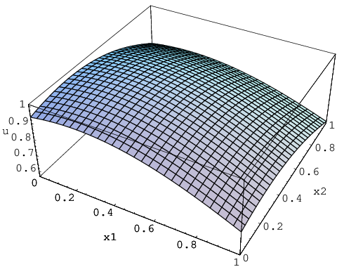
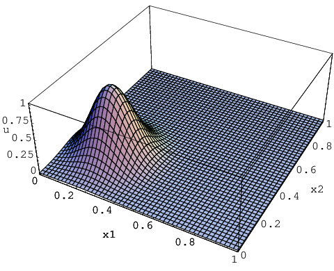
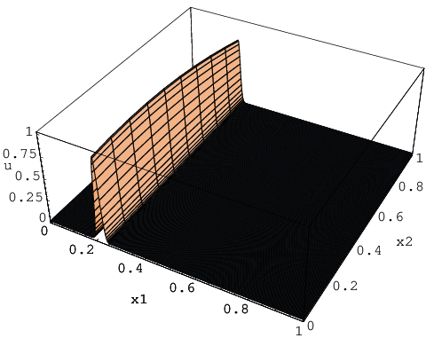
The evaluation point x∗x_{*} is chosen equal to the point pp. To illustrate the scales involved, we plot uu for a selection of parameters with fixed λ3=1\lambda_{3}=1 and for a cross-section x3=p3x_{3}=p_{3}.

Refer to caption
Refer to caption
Refer to caption
Figure 4: u⁡(x1,x2,p3)u(x_{1},x_{2},p_{3}) for (λ1,λ2,λ3)=(1,1,1)(\lambda_{1},\lambda_{2},\lambda_{3})=(1,1,1) (left), (λ1,λ2,λ3)=(100,100,1)(\lambda_{1},\lambda_{2},\lambda_{3})=(100,100,1) (middle) and (λ1,λ2,λ3)=(10000,1,1)(\lambda_{1},\lambda_{2},\lambda_{3})=(10000,1,1) (right).

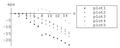
Fig. 5 shows how the error increases with increasing (mixed) derivatives.
Refer to caption
Figure 5: Pointwise sparse grid error ϵn\epsilon_{n} as in (64) on level nn for equation (62) with solution (63) for different values for λ1\lambda_{1}, λ2\lambda_{2} and λ3\lambda_{3}.

6.2 Parabolic and hyperbolic problems

We consider

ut−ν​Δ​u+𝐛⋅∇u=0u_{t}-\nu\Delta u+{\bf b}\cdot\nabla u=0

in two dimensions for different values of ν\nu. The case ν=0\nu=0 resembles the advection equation.

To adjust the smoothness, we choose an initial profile

u⁡(x1,x2,0)={1r<r¯,arctan⁡(tank⁡(π2​|r−r¯−ϵ|ϵ))r¯≤r≤r¯,0r>r¯,u(x_{1},x_{2},0)=\left\{\begin{array}[]{rl}1&\;\;\;r<\underline{r},\\ \arctan\left(\tan^{k}\left(\frac{\pi}{2}\frac{|r-\underline{r}-\epsilon|}{\epsilon}\right)\right)&\;\;\;\underline{r}\leq r\leq\overline{r},\\ 0&\;\;\;r>\overline{r},\end{array}\right.

where

r=(x1−m1)2+(x2−m2)2,\displaystyle r=\sqrt{(x_{1}-m_{1})^{2}+(x_{2}-m_{2})^{2}},

r¯=(1−ϵ)​r¯\underline{r}=(1-\epsilon)\overline{r} for ϵ∈[0,1]\epsilon\in[0,1] and k≥1k\geq 1 (see Fig. 6, left, for ϵ=0.9\epsilon=0.9).

The value is 1 in an inner circle with centre (m1,m2)(m_{1},m_{2}) and radius r¯\underline{r}, and changes to 0 within a distance of ϵ\epsilon. The regions are joined together such that k−1k-1 is the order of differentiability for ϵ>0\epsilon>0. ϵ=0\epsilon=0 is the discontinuous limit. We choose k=5k=5, because the analysis predicts that mixed derivatives of order up to 2+22+2 are required for upwinding on a sparse grid. Homogeneous Dirichlet conditions u=0u=0 are set at the boundary. To avoid any effects arising from the velocity being aligned with the grid, we choose b1=0.31415926535897932385b_{1}=0.31415926535897932385, b2=−0.27182818284590452354b_{2}=-0.27182818284590452354, we furthermore set m1=0.5​(1−b1)m_{1}=0.5(1-b_{1}), m2=0.5​(1−b2)m_{2}=0.5(1-b_{2}) and r¯=0.5​|𝐛|2\overline{r}=0.5|{\bf b}|_{2}, such that in the non-diffusive case the profile starts from the upper left quarter of the unit square, with the outer circle going through the centre (Fig. 6, left, for ϵ=0.9\epsilon=0.9), and is propagated down to the lower right quarter, touching the centre from the other side at T=1T=1. We evaluate the solution at the centre x∗=(1/2,…,1/2)x_{*}=(1/2,\ldots,1/2) and since the exact solution is unknown, we study the surplus

ϵ^n=|un+1​(x∗)−un​(x∗)|.\hat{\epsilon}_{n}=|u_{n+1}(x_{*})-u_{n}(x_{*})|. (67)

We first consider the setting ν=0.1\nu=0.1, ϵ=0.9\epsilon=0.9. The numerical solution is shown in Fig. 6.

Refer to caption
Refer to caption
Figure 6: Sparse grid solution at level n=15n=15 for ν=0.1,ϵ=0.9\nu=0.1,\epsilon=0.9 at t=0t=0 (left) and t=1t=1 (right).

First order convergence is observed as illustrated by Fig. 7.

Refer to caption
nn rn=ϵ^n/ϵ^n+1r_{n}=\hat{\epsilon}_{n}/\hat{\epsilon}_{n+1}
4 0.060907
5 0.25877
6 -4.2474
7 0.45337
8 2.0783
9 -2.8072
10 0.76331
11 1.2188
12 1.4628
13 1.5811
14 1.6559
15 1.7072
16 1.7449
17 1.7604
18 1.8364
Figure 7: ϵ^n\hat{\epsilon}_{n} as in (67) and convergence rate rnr_{n} at refinement level nn for ν=0.1\nu=0.1, ϵ=0.9\epsilon=0.9.

We now take ϵ=0\epsilon=0 and change ν=0.1,0.01,0.001\nu=0.1,0.01,0.001. (Fig. 8, left). Due to the discontinuous initial condition, the problem does not fit into the theoretical framework. Nonetheless, the smoothing property of the diffusion operator suffices to provide sufficient regularity for t>0t>0.

Alternatively, taking ν=0\nu=0, we let the smooth transition collapse to ϵ=0.1,0.01,0.001\epsilon=0.1,0.01,0.001 (Fig. 8, right).

Refer to caption
Refer to caption
Figure 8: Convergence of the sparse grid solution for discontinuous initial data for small diffusivity (left) and smooth initial data without diffusion (right) for with ϵ^n\hat{\epsilon}_{n} from (67).

Although the problem is sufficiently smooth, the scales involved are not resolved properly and the (mixed) derivatives are too large to reach the asymptotic range at feasible refinement levels.

Finally, consider the limiting case ν=0\nu=0, ϵ=0\epsilon=0, i.e. a discontinuous initial profile without diffusion.

Refer to caption
Refer to caption
Figure 9: Sparse grid solution at level n=15n=15 for ν=0,ϵ=0\nu=0,\epsilon=0 at t=0t=0 (left) and t=1t=1 (right).

Already in Fig. 9 the problems of the sparse grid become apparent. It is noticeable how the anisotropic elements in the sparse grid fail to capture the discontinuous transition at the circumference of the circle. Fig. 10 confirms that convergence (if any) is slow and erratic.

Refer to caption
nn rn=ϵ^n/ϵ^n+1r_{n}=\hat{\epsilon}_{n}/\hat{\epsilon}_{n+1}
4 2.0381
5 1.0974
6 0.85633
7 -0.61664
8 1.7166
9 -6.8473
10 0.29471
11 0.87042
12 1.9361
13 2.4390
14 -5.2997
15 -0.64137
16 -0.43160
17 0.38301
18 1.58094
Figure 10: ϵ^n\hat{\epsilon}_{n} as in (67) and convergence rate rnr_{n} at refinement level nn for discontinuous initial data without diffusion.

7 Discussion

In this article, we give explicit error bounds for the sparse grid combination solution to model problems in a finite difference context, and at the same time provide a framework that can be applied to more general linear PDEs. The ingredients are:

  1. 1.

    sufficiently smooth and compatible data to yield solutions with bounded mixed derivatives of required order;

  2. 2.

    a discretisation scheme that provides a truncation error of certain mixed order;

  3. 3.

    stability of the discretisation scheme, i.e. a bounded inverse in the maximum norm.

In most cases, the truncation error can be assessed easily by Taylor expansion. The boundedness of the inverse will be harder to establish, but note that no additional requirements to the corresponding full grid case are necessary in this regard. Examples that fall into this category, e.g. where discrete maximum principles are known, are elliptic and parabolic equations. The numerical results reproduce the theoretical findings nicely.

Limitations we encountered concern non-smooth problems, dimensions in excess of eight, and non-diagonal diffusion tensors. The latter can often be resolved in practice by diagonalising the diffusion tensor and performing a principal component or asymptotic analysis, see e.g. (Reisinger and Wittum 2007).

Acknowledgements

The author wishes to thank Mike Giles for illuminating discussions on the subject, in particular for pointing him towards the concept of adjoint error correction (Giles and Süli 2002), which proved vital for the theory of Section 3; Endre Süli and Tony Ware for advice on questions regarding the regularity of solutions, which were raised by an anonymous referee of an earlier version of this manuscript whose contribution in spotting this is also gratefully acknowledged.

References

  • Bachmayr [2010] M. Bachmayr. Hyperbolic wavelet discretization of the two-electron Schrödinger equation in an explicitly correlated formulation. AICES Preprint 2010/06-2, RWTH Aachen, June 2010.
  • Bungartz [1992] H.-J. Bungartz. Dünne Gitter und deren Anwendung bei der adaptiven Lösung der dreidimensionalen Poisson-Gleichung. PhD thesis, Technische Universität München, 1992.
  • Bungartz [1998] H.-J. Bungartz. Finite elements of higher order on sparse grids. Habilitationsschrift, Technische Universität München, 1998.
  • Bungartz and Griebel [2004] H.-J. Bungartz and M. Griebel. Sparse grids. Acta Numerica, 13:1–123, 2004.
  • Bungartz et al. [1994] H.-J. Bungartz, M. Griebel, D. Röschke, and C. Zenger. Pointwise convergence of the combination technique for the Laplace equation. East-West J. Num. Math., 2:21–45, 1994.
  • Dauge and Stevenson [2010] M. Dauge and R. Stevenson. Sparse tensor product wavelet approximation of singular functions. SIAM J. Math. Anal., 42(5):2203–2228, 2010.
  • Dijkema et al. [2009] T. J. Dijkema, C. Schwab, and R. Stevenson. An adaptive wavelet method for solving high-dimensional elliptic PDEs. Constr. Approx., 30(3):423–455, 2009.
  • Garcke and Griebel [2000] J. Garcke and M. Griebel. On the computation of the eigenproblems of hydrogen and helium in strong magnetic and electric fields with the sparse grid combination technique. Journal of Computational Physics, 165(2), 2000.
  • Gerstner and Griebel [2003] T. Gerstner and M. Griebel. Dimension–Adaptive Tensor–Product Quadrature. Computing, 71(1):65–87, 2003.
  • Gerstner et al. [2009] T. Gerstner, M. Griebel, and M. Holtz. Efficient deterministic numerical simulation of stochastic asset-liability management models in life insurance. Insurance: Math. Economics, 44:434–446, 2009.
  • Giles and Süli [2002] M.B. Giles and E. Süli. Adjoint methods for PDEs: a posteriori error analysis and postprocessing by duality. Acta Numerica, pages 145–236, 2002.
  • Griebel [2006] M. Griebel. Sparse grids and related approximation schemes for higher dimensional problems. In L.-M. Pardo, A. Pinkus, E. Süli, and M. Todd, editors, Foundations of Computational Mathematics 2005, pages 106–161. Cambridge University Press, 2006.
  • Griebel and Hamaekers [2007] M. Griebel and J. Hamaekers. Sparse grids for the Schrödinger equation. ESAIM: Mathematical Modelling and Numerical Analysis, 41(2):215–247, 2007.
  • Griebel and Holtz [2010] M. Griebel and M. Holtz. Dimension-wise integration of high-dimensional functions with applications to finance. J. Complexity, 26(5):455–489, 2010.
  • Griebel and Thurner [1995] M. Griebel and V. Thurner. The efficient solution of fluid dynamics problems by the combination technique. Int. J. Num. Meth. for Heat and Fluid Flow, 1995.
  • Griebel et al. [1992] M. Griebel, M. Schneider, and C. Zenger. A combination technique for the solution of sparse grid problems. In P. de Groen and R. Beauwens, editors, Iterative Methods in Linear Algebra. IMACS, Elsevier, North Holland, 1992.
  • Hegland [2003] M. Hegland. Adaptive sparse grids. In K. Burrage and Roger B. Sidje, editors, Proc. of 10th Computational Techniques and Applications Conference CTAC-2001, volume 44, pages 335–353, 2003.
  • Hilber et al. [2005] N. Hilber, A.M. Matache, and C. Schwab. Sparse wavelet methods for option pricing under stochastic volatility. J. Comp. Fin., 8(4):1–42, 2005.
  • Kangro and Nicolaides [2001] R. Kangro and R. Nicolaides. Far field boundary conditions for Black-Scholes equations. SIAM J. Numer. Anal., 38(4):1357–1368, 2001.
  • Leentvaar and Oosterlee [2008] C.C.W. Leentvaar and C.W. Oosterlee. On coordinate transformation and grid stretching for sparse grid pricing of basket options. J. Comp. Appl. Math., 222:193–209, 2008.
  • Nitsche [2005] P.-A. Nitsche. Sparse approximation of singularity functions. Constr. Approx., 21:63Ð81, 2005.
  • Novak and Ritter [1996] E. Novak and K. Ritter. High dimensional integration of smooth functions over cubes. Numer. Math., 75(1):79–98, 1996.
  • Pflaum [1997] C. Pflaum. Convergence of the combination technique for second-order elliptic differential equations. SIAM J. Numer. Anal., 34(6):2431–2455, December 1997.
  • Pflaum and Zhou [1999] C. Pflaum and A. Zhou. Error analysis of the combination technique. Numerische Mathematik, 84:327–350, December 1999.
  • Reisinger [2004] C. Reisinger. Efficient Numerical Methods for High-Dimensional Parabolic Equations and Applications in Option Pricing. PhD thesis, Universität Heidelberg, 2004.
  • Reisinger and Wittum [2007] C. Reisinger and G. Wittum. Efficient hierarchical approximation of high-dimensional option pricing problems. SIAM J. Sci. Comp., 29(1), 2007.
  • Schwab et al. [2008] C. Schwab, E. Süli, and R.-A. Todor. Sparse finite element approximation of high-dimensional transport-dominated diffusion problems. ESAIM: Mathematical Modelling and Numerical Analysis, 42(5):777–820, 2008.
  • Smolyak [1963] S. Smolyak. Quadrature and interpolation formulas for tensor products of certain classes of functions. Soviet Math. Dokl., 4:240Ð243, 1963.
  • von Petersdorff and Schwab [2004] T. von Petersdorff and C. Schwab. Numerical solution of parabolic equations in high dimensions. ESAIM: Mathematical Modelling and Numerical Analysis, 38(1):93–127, 2004.
  • Wloka [1987] J. Wloka. Partial differential equations. Cambridge University Press, 1987.
  • Yserentant [2010] H. Yserentant. Regularity and Approximability of Electronic Wave Functions. Number 2000 in Lecture Notes in Mathematics. Springer, 2010.
  • Zeiser [2010] A. Zeiser. Wavelet approximation in weighted Sobolev spaces of mixed order with applications to the electronic Schrödinger equation. SPP 1324 Preprint, TU Berlin, July 2010.
  • Zenger [1990] C. Zenger. Sparse grids. In W. Hackbusch, editor, Parallel Algorithms for Partial Differential Equations, volume 31 of Notes on Numerical Fluid Dynamics, 1990. Proceedings of the Sixth GAMM-Seminar.

Appendix A Smoothness of solutions to the Poisson problem on the hyper-cube

A.1 Fourier series expansion

In this section, we derive a sufficient condition on the decay of the Fourier (sine) coefficients of the right-hand side ff, in order for the solution uu to the Poisson problem (29) to have sufficient regularity.

Theorem A.1.

Let f𝐤f_{{\bf k}} be the coefficients of ff in a sine-series with multi-index 𝐤=(k1,…,kd)∈ℕd{\bf k}=(k_{1},\ldots,k_{d})\in\mathbb{N}^{d}. Then if

∑𝐤∑𝐢,|𝐢|1≤⌈d/2⌉k18+i1⋅…⋅kd8+id(k12+…+kd2)2​f𝐤2<∞,\sum_{{\bf k}}\sum_{{\bf i},|{\bf i}|_{1}\leq\lceil d/2\rceil}\frac{k_{1}^{8+i_{1}}\cdot\ldots\cdot k_{d}^{8+i_{d}}}{\left(k_{1}^{2}+\ldots+k_{d}^{2}\right)^{2}}f_{{\bf k}}^{2}<\infty,

the solution uu to the Poisson problem has regularity

u∈X4du\in X_{4}^{d}

with X4dX_{4}^{d} defined in (13) as the space of all functions with continuous mixed derivatives up to order 4 that vanish at the boundaries.

Proof.

Expanding both ff and uu into sin\sin-series,

f⁡(𝐱)\displaystyle f({\bf x}) =\displaystyle= ∑𝐤f𝐤​∏j=1dsin⁡(π​kj​xj)\displaystyle\sum_{{\bf k}}f_{{\bf k}}\prod_{j=1}^{d}\sin(\pi k_{j}x_{j})
u⁡(𝐱)\displaystyle u({\bf x}) =\displaystyle= ∑𝐤u𝐤​∏j=1dsin⁡(π​kj​xj)\displaystyle\sum_{{\bf k}}u_{{\bf k}}\prod_{j=1}^{d}\sin(\pi k_{j}x_{j})

then for the Fourier coefficients u𝐤u_{{\bf k}} and f𝐤f_{{\bf k}}

u𝐤=f𝐤|𝐤|22.u_{{\bf k}}=\frac{f_{{\bf k}}}{|{\bf k}|_{2}^{2}}.

Norm equivalence gives

f∈L2\displaystyle f\in L_{2} ⇔\displaystyle\Leftrightarrow ∑𝐤f𝐤2<∞\displaystyle\sum_{{\bf k}}f_{{\bf k}}^{2}<\infty
∂4​df∂x14​…​∂xd4∈L2\displaystyle\frac{\partial^{4d}f}{\partial x_{1}^{4}\ldots\partial x_{d}^{4}}\in L_{2} ⇔\displaystyle\Leftrightarrow ∑𝐤[k14⋅…⋅kd4​f𝐤]2<∞\displaystyle\sum_{{\bf k}}\left[k_{1}^{4}\cdot\ldots\cdot k_{d}^{4}f_{{\bf k}}\right]^{2}<\infty
∂4​du∂x14​…​∂xd4∈L2\displaystyle\frac{\partial^{4d}u}{\partial x_{1}^{4}\ldots\partial x_{d}^{4}}\in L_{2} ⇔\displaystyle\Leftrightarrow ∑𝐤[k14⋅…⋅kd4k12+…+kd2]2​f𝐤2<∞\displaystyle\sum_{{\bf k}}\left[\frac{k_{1}^{4}\cdot\ldots\cdot k_{d}^{4}}{k_{1}^{2}+\ldots+k_{d}^{2}}\right]^{2}f_{{\bf k}}^{2}<\infty

Further, see e.g. [Wloka 1987], Theorem 6.2, p. 107, W2k↪ClW_{2}^{k}\hookrightarrow C^{l} for k−l≥d/2k-l\geq d/2, in particular

W2k↪C​ for ​k≥d/2.W_{2}^{k}\hookrightarrow C\text{ for }k\geq d/2.

From this the statement follows. ∎

A.2 Maximum norm of mixed derivatives

Theorem A.2.

For the Poisson problem (29), if continuous derivatives up to the relevant order exist, then

‖∂k14…​∂km4u‖∞≤18​‖∂k14…​∂km4f‖∞+∑i=1d‖∂k14…​∂km4∂i2f‖∞.\|\partial_{k_{1}}^{4}\ldots\partial_{k_{m}}^{4}u\|_{\infty}\leq\frac{1}{8}\|\partial_{k_{1}}^{4}\ldots\partial_{k_{m}}^{4}f\|_{\infty}+\sum_{i=1}^{d}\|\partial_{k_{1}}^{4}\ldots\partial_{k_{m}}^{4}\partial_{i}^{2}f\|_{\infty}.
Proof.

In order to get bounds on the derivative norms, we derive PDEs and boundary conditions for mixed (fourth) derivatives, by differentiating the PDE, and can then apply a maximum principle argument. From ∑i=1d∂i2u=f\sum_{i=1}^{d}\partial_{i}^{2}u=f follows

∑i=1d∂i2(∂k14…​∂kd4u)=∂k14…​∂kd4f,\sum_{i=1}^{d}\partial_{i}^{2}\left(\partial_{k_{1}}^{4}\ldots\partial_{k_{d}}^{4}u\right)=\partial_{k_{1}}^{4}\ldots\partial_{k_{d}}^{4}f, (68)

and therefore derivatives of the solution satisfy a Poisson problem with the right-hand side a derivative of the original one. We now derive boundary conditions for ∂k14…​∂kd4u\partial_{k_{1}}^{4}\ldots\partial_{k_{d}}^{4}u at x1=0x_{1}=0. The other cases follow by permutation and symmetry. From

∂iku=0​ for ​i>1,k≥0\partial_{i}^{k}u=0\text{ for }i>1,\;k\geq 0

follows

∂12u=∂12u+∑i=2d∂i2u=f,\partial_{1}^{2}u=\partial_{1}^{2}u+\sum_{i=2}^{d}\partial_{i}^{2}u=f,

and from ∂i2∂j2u=0\partial_{i}^{2}\partial_{j}^{2}u=0 for i,j>1i,j>1

∂12∂j2u=∂12∂j2u+∑i=2d∂i2∂j2u=∂j2f\partial_{1}^{2}\partial_{j}^{2}u=\partial_{1}^{2}\partial_{j}^{2}u+\sum_{i=2}^{d}\partial_{i}^{2}\partial_{j}^{2}u=\partial_{j}^{2}f

for j>1j>1. Also,

∂14u+∑i=2d∂12∂i2u=∂12f,\partial_{1}^{4}u+\sum_{i=2}^{d}\partial_{1}^{2}\partial_{i}^{2}u=\partial_{1}^{2}f,

and consequently for 2≤k1,…,km≤d2\leq k_{1},\ldots,k_{m}\leq d

∂k14…​∂km4∂14u=∂k14…​∂km4∂12f−∑i=2d∂k14…​∂km4∂i2f\partial_{k_{1}}^{4}\ldots\partial_{k_{m}}^{4}\partial_{1}^{4}u=\partial_{k_{1}}^{4}\ldots\partial_{k_{m}}^{4}\partial_{1}^{2}f-\sum_{i=2}^{d}\partial_{k_{1}}^{4}\ldots\partial_{k_{m}}^{4}\partial_{i}^{2}f (69)

for x1=0x_{1}=0. All other mixed derivatives without x1x_{1} in them are zero at this boundary face.

From (68) and (69) the result follows by a maximum principle argument. ∎

Appendix B Proofs from Section 4

Proof of Lemma 4.1.

Define

v\displaystyle v :⁣=\displaystyle:= u⁡(x1,…,xd)−u⁡(0,…,0)−∑i=1dxi​∂iu⁡(x−x(i))−∑i,j=1i≠jdxi​xj​∂i∂ju⁡(x−x(i,j))−…−\displaystyle u(x_{1},\ldots,x_{d})-u(0,\ldots,0)-\sum_{i=1}^{d}x_{i}\,\partial_{i}u(x-x^{(i)})\;-\sum_{\scriptsize\begin{array}[]{c}i,j=1\\ i\neq j\end{array}}^{d}x_{i}x_{j}\,\partial_{i}\partial_{j}u(x-x^{(i,j)})-\ldots-
−x1⋅…⋅xd∂1…∂du|x1,…,xd=0−∑i=1d∫0xi(xi−si)∂i2u(s(i))dsi−…−\displaystyle\hskip-25.6073pt-\;x_{1}\cdot\ldots\cdot x_{d}\left.\partial_{1}\ldots\partial_{d}u\right|_{x_{1},\ldots,x_{d}=0}\;-\;\sum_{i=1}^{d}\int_{0}^{x_{i}}(x_{i}-s_{i})\,\partial_{i}^{2}u(s^{(i)})\,\text{\rm d$s$}_{i}-\ldots-
−∑{i1,…,id−1}⊂{1,…,d}∫0xi1…∫0xid−1(xi1−si1)⋅…⋅(xid−1−sid−1)∂i12…∂id−12u(s(i1,…,id−1))dsid−1…dsi1.\displaystyle\hskip-25.6073pt-\hskip-14.22636pt\sum_{\scriptsize\begin{array}[]{c}\{i_{1},\ldots,i_{d-1}\}\\ \subset\{1,\ldots,d\}\end{array}}\!\!\int_{0}^{x_{i_{1}}}\ldots\int_{0}^{x_{i_{d-1}}}\!(x_{i_{1}}-s_{i_{1}})\cdot\ldots\cdot(x_{i_{d-1}}-s_{i_{d-1}})\partial_{i_{1}}^{2}\ldots\partial_{i_{d-1}}^{2}u(s^{(i_{1},\ldots,i_{d-1})})\,\,\text{\rm d$s$}_{i_{d-1}}\ldots\,\text{\rm d$s$}_{i_{1}}.

It is straightforward to see that

v⁡(x1,…,xd)=0if∃k:xk=0v(x_{1},\ldots,x_{d})=0\quad{\rm if}\quad\exists k:\;x_{k}=0

and also

D𝜶​v​(x1,…,xd)=0if∃k:xk=0∧αk=1.D^{\boldsymbol{\alpha}}v(x_{1},\ldots,x_{d})=0\quad{\rm if}\quad\exists k:\;x_{k}=0\;\wedge\;\alpha_{k}=1.

From

∂12…​∂d2v=0\partial_{1}^{2}\ldots\partial_{d}^{2}v=0

one gets v=0v=0 from which the result follows. ∎

Proof of Theorem 4.2.

Without loss of generality consider a point xx in the box B:=[0,h1]×…×[0,hd]B:=[0,h_{1}]\times\ldots\times[0,h_{d}]. For all corner points p=(p1,…,pd)∈Bc:=⨂i=1d{0,hi}p=(p_{1},\ldots,p_{d})\in B_{c}:=\bigotimes_{i=1}^{d}\{0,h_{i}\} use Lemma 4.1 to express

u⁡(p)\displaystyle u(p) =\displaystyle= u⁡(x)+∑i=1d(pi−xi)​∂iu⁡(x(i))+∑i,j=1i≠jd(pi−xi)​(pj−xj)​∂i∂ju⁡(x(i,j))+…+\displaystyle u(x)+\sum_{i=1}^{d}(p_{i}-x_{i})\partial_{i}u(x^{(i)})+\sum_{\scriptsize\begin{array}[]{c}i,j=1\\ i\neq j\end{array}}^{d}(p_{i}-x_{i})(p_{j}-x_{j})\partial_{i}\partial_{j}u(x^{(i,j)})+\ldots+\vskip-28.45274pt (75)
+(p1−x1)⋅…⋅(pd−xd)∂1…∂du(x)+∑i=1d∫xipi(pi−si)∂i2u(s(i))dsi+…+\displaystyle\hskip-28.45274pt+\;(p_{1}-x_{1})\cdot\ldots\cdot(p_{d}-x_{d})\partial_{1}\ldots\partial_{d}u(x)\;+\;\sum_{i=1}^{d}\int_{x_{i}}^{p_{i}}(p_{i}-s_{i})\partial_{i}^{2}u(s^{(i)})\,\text{\rm d$s$}_{i}+\ldots+
+∫x1p1…∫xdpd(p1−s1)⋅…⋅(pd−sd)∂12…∂d2u(s)dsd…ds1\displaystyle\hskip-28.45274pt+\;\int_{x_{1}}^{p_{1}}\ldots\int_{x_{d}}^{p_{d}}(p_{1}-s_{1})\cdot\ldots\cdot(p_{d}-s_{d})\,\partial_{1}^{2}\ldots\partial_{d}^{2}u(s)\,\text{\rm d$s$}_{d}\ldots\,\text{\rm d$s$}_{1}

Here x=(x1,…,xd)x=(x_{1},\ldots,x_{d}), and introduce x(i1,…,ik),s(i1,…,ik)∈ℝdx^{(i_{1},\ldots,i_{k})},s^{(i_{1},\ldots,i_{k})}\in\mathbb{R}^{d} with xj(i1,…,ik)=xjx^{(i_{1},\ldots,i_{k})}_{j}=x_{j} if j∈{i1,…​ik}j\in\{i_{1},\ldots i_{k}\}, pjp_{j} otherwise, and sj(i1,…,ik)=sjs^{(i_{1},\ldots,i_{k})}_{j}=s_{j} if j∈{i1,…​ik}j\in\{i_{1},\ldots i_{k}\}, xjx_{j} otherwise.

Then insert in the multilinear approximation

(ℐ​u​(𝐱h))​(x)=∑p∈Bc|p1−x1|h1⋅…⋅|pd−xd|hd⋅u⁡(p)=u⁡(x)+∑m=1d∑{i1,…,im}⊂{1,…,d}∑p∈Bcwi1,…,im​(p,x)\displaystyle(\mathcal{I}u({\bf x}_{h}))(x)=\sum_{p\in B_{c}}\frac{|p_{1}-x_{1}|}{h_{1}}\cdot\ldots\cdot\frac{|p_{d}-x_{d}|}{h_{d}}\cdot u(p)=u(x)+\sum_{m=1}^{d}\!\!\sum_{\tiny\begin{array}[]{c}\{i_{1},\ldots,i_{m}\}\\ \subset\{1,\ldots,d\}\end{array}}\!\!\sum_{p\in B_{c}}w_{i_{1},\ldots,i_{m}}(p,x)

with

wi1,…,im​(p,x)=(∏k=1d|pk−xk|hk)​∫xi1pi1…​∫ximpim(∏k=1m(pik−sik))​∂i12…​∂im2u⁡(s(i1,…,im))​dsim​…​dsi1,\displaystyle w_{i_{1},\ldots,i_{m}}(p,x)=\left(\prod_{k=1}^{d}\frac{|p_{k}-x_{k}|}{h_{k}}\right)\int_{x_{i_{1}}}^{p_{i_{1}}}\!\!\ldots\int_{x_{i_{m}}}^{p_{i_{m}}}\!\left(\prod_{k=1}^{m}(p_{i_{k}}-s_{i_{k}})\right)\,\partial_{i_{1}}^{2}\ldots\partial_{i_{m}}^{2}u(s^{(i_{1},\ldots,i_{m})})\,\text{\rm d$s$}_{i_{m}}\ldots\,\text{\rm d$s$}_{i_{1}},

because all the terms in (75) that are multilinear are exactly represented. By inserting the points p∈Bcp\in B_{c} one shows after some calculation the representation

αj1,…,jm​(x,hj1,…,hjm)=∏k=1mxjkhjk​(1−xjkhjk)​∑𝐲,𝐳∈{0,1}myk+zk=1k=1,…,m∏k=1m(xjkhjk)yk​(1−xjkhjk)zk​w𝐲,𝐳​(x,𝐡)\alpha_{j_{1},\ldots,j_{m}}(x;h_{j_{1}},\ldots,h_{j_{m}})=\prod_{k=1}^{m}\frac{x_{j_{k}}}{h_{j_{k}}}\left(1-\frac{x_{j_{k}}}{h_{j_{k}}}\right)\!\!\sum_{\scriptsize\begin{array}[]{c}{\bf y},{\bf z}\in\{0,1\}^{m}\\ y_{k}+z_{k}=1\\ k=1,\ldots,m\end{array}}\prod_{k=1}^{m}\left(\frac{x_{j_{k}}}{h_{j_{k}}}\right)^{\!y_{k}}\!\left(1-\frac{x_{j_{k}}}{h_{j_{k}}}\right)^{\!z_{k}}w_{{\bf y},{\bf z}}(x;{\bf h}) (77)

with 𝐡=(hi1,…,him){\bf h}=(h_{i_{1}},\ldots,h_{i_{m}}) and

w𝐲,𝐳​(x,𝐡)=1∏k=1dxk2​yk​(hjk−xk)2​zk​∫x1z1​hj1…​∫xmzm​hjm(∏k=1m(zk​hjk−sk))​∂12…​∂m2u⁡(s(j1,…,jm))​dsm​…​ds1.w_{{\bf y},{\bf z}}(x;{\bf h})=\frac{1}{\prod\limits_{k=1}^{d}x_{k}^{2y_{k}}(h_{j_{k}}-x_{k})^{2z_{k}}}\int_{x_{1}}^{z_{1}h_{j_{1}}}\!\!\ldots\int_{x_{m}}^{z_{m}h_{j_{m}}}\left(\prod_{k=1}^{m}(z_{k}h_{j_{k}}-s_{k})\right)\partial_{1}^{2}\ldots\partial_{m}^{2}u(s^{(j_{1},\ldots,j_{m})})\,\text{\rm d$s$}_{m}\ldots\,\text{\rm d$s$}_{1}.

The rest follows because the maximum of ξ2​(1−ξ)\xi^{2}(1-\xi) on [0,1][0,1] is 427\frac{4}{27}. ∎

Proof of Theorem 4.3.

From Corollary 3.4 wi1,…,ik​(𝐱h,hi1,…,hik)w_{i_{1},\ldots,i_{k}}({\bf x}_{h};h_{i_{1}},\ldots,h_{i_{k}}) (in (49)) is the restriction of a function wi1,…,ikw_{i_{1},\ldots,i_{k}} from hyperplanes 𝐈h(i1,…,ik){\bf I}_{h}^{(i_{1},\ldots,i_{k})} to the grid 𝐱h{\bf x}_{h}, where for the derivatives in the continuous directions

‖D𝜶​wi1,…,ik​(⋅,hi1,…,hik)‖0≤k!48k​‖D𝜷​u‖∞\|D^{\boldsymbol{\alpha}}w_{i_{1},\ldots,i_{k}}(\cdot;h_{i_{1}},\ldots,h_{i_{k}})\|_{0}\leq\frac{k!}{48^{k}}\|D^{\boldsymbol{\beta}}u\|_{\infty}

with αi=4\alpha_{i}=4, i∉{i1,…,ik}i\notin\{i_{1},\ldots,i_{k}\} βi=4\beta_{i}=4 holds.

By Theorem 4.2 for points xx on the hyper-planes 𝐈h(i1,…,ik){\bf I}_{h}^{(i_{1},\ldots,i_{k})}

(ℐ​wi1,…,ik​(𝐱h,hi1,…,hik))​(x)\displaystyle(\mathcal{I}w_{i_{1},\ldots,i_{k}}({\bf x}_{h};h_{i_{1}},\ldots,h_{i_{k}}))(x) =\displaystyle= wi1,…,ik​(x,hi1,…,hik)+\displaystyle w_{i_{1},\ldots,i_{k}}(x;h_{i_{1}},\ldots,h_{i_{k}})+
∑{j1,…,jm}∩{i1,…,ik}=∅γi1,…,ik;j1,…,jm​(x,hi1,…,hik,hj1,…,hjm)​hj12⋅…⋅hjm2\displaystyle\hskip-113.81102pt\sum_{\scriptsize\begin{array}[]{c}\{j_{1},\ldots,j_{m}\}\\ \cap\{i_{1},\ldots,i_{k}\}=\emptyset\end{array}}\gamma_{i_{1},\ldots,i_{k};j_{1},\ldots,j_{m}}(x,h_{i_{1}},\ldots,h_{i_{k}};h_{j_{1}},\ldots,h_{j_{m}})h_{j_{1}}^{2}\cdot\ldots\cdot h_{j_{m}}^{2}

with |γi1,…,ik;j1,…,jm​(x,hi1,…,hik,hj1,…,hjm)|≤4m27m​‖D𝜶​w‖∞|\gamma_{i_{1},\ldots,i_{k};j_{1},\ldots,j_{m}}(x;h_{i_{1}},\ldots,h_{i_{k}};h_{j_{1}},\ldots,h_{j_{m}})|\leq\frac{4^{m}}{27^{m}}\|D^{\boldsymbol{\alpha}}w\|_{\infty} where αil=4,αjn=2\alpha_{i_{l}}=4,\alpha_{j_{n}}=2. Values between the hyperplanes are obtained by multilinear interpolation, which introduces no new maxima, and thus

ℐ⁡(u⁡(𝐱h)−𝐮h)\displaystyle\mathcal{I}(u({\bf x}_{h})-{\bf u}_{h}) =\displaystyle= ∑{i1,…,ik}⊂{1,…,k}βi1,…,ik​(⋅,hi1,…,hik)​hi12⋅…⋅hik2+\displaystyle\!\!\sum_{\scriptsize\begin{array}[]{c}\{i_{1},\ldots,i_{k}\}\\ \subset\{1,\ldots,k\}\end{array}}\!\!\beta_{i_{1},\ldots,i_{k}}(\cdot;h_{i_{1}},\ldots,h_{i_{k}})h_{i_{1}}^{2}\cdot\ldots\cdot h_{i_{k}}^{2}+
+∑{j1,…,jm}∩{i1,…,ik}=∅βi1,…,ik;j1,…,jm(⋅;hi1,…,hik;hj1,…,hjm)hi12⋅…⋅hik2⋅hj12⋅…⋅hjm2\displaystyle\hskip-85.35826pt+\!\!\sum_{\scriptsize\begin{array}[]{c}\{j_{1},\ldots,j_{m}\}\\ \cap\{i_{1},\ldots,i_{k}\}=\emptyset\end{array}}\!\!\!\!\!\!\!\!\beta_{i_{1},\ldots,i_{k};j_{1},\ldots,j_{m}}(\cdot;h_{i_{1}},\ldots,h_{i_{k}};h_{j_{1}},\ldots,h_{j_{m}})h_{i_{1}}^{2}\cdot\ldots\cdot h_{i_{k}}^{2}\cdot h_{j_{1}}^{2}\cdot\ldots\cdot h_{j_{m}}^{2}

with ‖βi1,…,ik;j1,…,jm​(⋅,hi1,…,hik,hj1,…,hjm)‖∞≤K​k!96k​4m27m.\|\beta_{i_{1},\ldots,i_{k};j_{1},\ldots,j_{m}}(\cdot;h_{i_{1}},\ldots,h_{i_{k}};h_{j_{1}},\ldots,h_{j_{m}})\|_{\infty}\leq K\frac{k!}{96^{k}}\frac{4^{m}}{27^{m}}.

Putting (B) and (47) together one gets

u−ℐ​𝐮h=∑m=1d∑{j1,…,jm}⊂{1,…,d}vj1,…,jm​(⋅,hj1,…,hjm)​hj12⋅…⋅hjm2u-\mathcal{I}{\bf u}_{h}=\sum_{m=1}^{d}\sum_{\tiny\begin{array}[]{c}\{j_{1},\ldots,j_{m}\}\\ \subset\{1,\ldots,d\}\end{array}}v_{j_{1},\ldots,j_{m}}(\cdot;h_{j_{1}},\ldots,h_{j_{m}})h_{j_{1}}^{2}\cdot\ldots\cdot h_{j_{m}}^{2}

with

‖vj1,…,jm​(⋅,hj1,…,hjm)‖∞\displaystyle\|v_{j_{1},\ldots,j_{m}}(\cdot;h_{j_{1}},\ldots,h_{j_{m}})\|_{\infty} ≤\displaystyle\leq K​4m27m+K​m!96m+K​∑l=1m−1(ml)​(427)l​(m−l)!96(m−l)\displaystyle K\frac{4^{m}}{27^{m}}+K\frac{m!}{96^{m}}+K\sum_{l=1}^{m-1}\left(\begin{array}[]{c}m\\ l\end{array}\right)\left(\frac{4}{27}\right)^{l}\frac{(m-l)!}{96^{(m-l)}}
=\displaystyle= K​∑l=0m(ml)​(427)l​(m−l)!96m−l=K​m!96m​∑l=0m1l!​(38427)l\displaystyle K\sum_{l=0}^{m}\left(\begin{array}[]{c}m\\ l\end{array}\right)\left(\frac{4}{27}\right)^{l}\frac{(m-l)!}{96^{m-l}}=K\frac{m!}{96^{m}}\sum_{l=0}^{m}\frac{1}{l!}\left(\frac{384}{27}\right)^{l}
<\displaystyle< K​m!96m​e384/27<150188​K​m!96m.\displaystyle K\frac{m!}{96^{m}}{\rm e}^{384/27}<150188\,K\frac{m!}{96^{m}}.

∎

Proof of Theorem 4.4.

Follows by combining Theorems 3.5 and 4.2 similarly to the Poisson case by observing that one can write second order terms (from the bilinear interpolation) as first order terms by defining

βi1,…,ik​(⋅,hi1,…,hik)​hi12⋅…⋅hik2=:β^i1,…,ik​(⋅,hi1,…,hik)​hi1⋅…⋅hik\beta_{i_{1},\ldots,i_{k}}(\cdot;h_{i_{1}},\ldots,h_{i_{k}})h_{i_{1}}^{2}\cdot\ldots\cdot h_{i_{k}}^{2}=:\hat{\beta}_{i_{1},\ldots,i_{k}}(\cdot;h_{i_{1}},\ldots,h_{i_{k}})h_{i_{1}}\cdot\ldots\cdot h_{i_{k}}

with |β^i1,…,ik|≤|βi1,…,ik||\hat{\beta}_{i_{1},\ldots,i_{k}}|\leq|\beta_{i_{1},\ldots,i_{k}}| and the final estimate becomes

‖vj1,…,jm​(⋅,hj1,…,hjm)‖∞≤K​m!2m​∑l=0m1l!​(827)l≤K​m!2m​e8/27≤32​K​m!2m.\|v_{j_{1},\ldots,j_{m}}(\cdot;h_{j_{1}},\ldots,h_{j_{m}})\|_{\infty}\leq K\frac{m!}{2^{m}}\sum_{l=0}^{m}\frac{1}{l!}\left(\frac{8}{27}\right)^{l}\leq K\frac{m!}{2^{m}}{\rm e}^{8/27}\leq\frac{3}{2}K\frac{m!}{2^{m}}.

∎

Appendix C Proofs from Section 5

Proof of Lemma 5.3.

Inserting gives

F⁡(n)=∑|𝐢|=nv⁡(2−i1,…,2−im)​2−p​i1⋅…⋅2−p​im=\displaystyle F(n)=\hbox to0.0pt{$\displaystyle\sum_{|{\bf i}|=n}v(2^{-i_{1}},\ldots,2^{-i_{m}})2^{-pi_{1}}\cdot\ldots\cdot 2^{-pi_{m}}=$\hss}\hskip 56.9055pt
=\displaystyle= ∑|𝐢|=nv(2−i1,…,2−im)2−p∑k=1mik\displaystyle\sum_{|{\bf i}|=n}v(2^{-i_{1}},\ldots,2^{-i_{m}})2^{-p\sum_{k=1}^{m}i_{k}}
=\displaystyle= ∑l=0n∑∑k=1mik=lv⁡(2−i1,…,2−im)⏟=:sl2−p​l∑∑k=m+1dik=n−l1\displaystyle\sum_{l=0}^{n}\underbrace{\sum_{\sum_{k=1}^{m}i_{k}=l}v(2^{-i_{1}},\ldots,2^{-i_{m}})}_{=:s_{l}}2^{-pl}\sum_{\sum_{k=m+1}^{d}i_{k}=n-l}1
=\displaystyle= ∑l=0nsl​2−p​l​(n−l+d−m−1d−m−1).\displaystyle\sum_{l=0}^{n}s_{l}2^{-pl}\left(\begin{array}[]{c}n-l+d-m-1\\ d-m-1\end{array}\right).

From Lemma C.1 below, 2. (d→d−md\rightarrow d-m, fl→sl​2−p​lf_{l}\rightarrow s_{l}2^{-pl}) one obtains

δ1d−m​F​(n)=δ1d−m​∑|𝐢|=nv⁡(2−i1,…,2−im)​2−p​i1⋅…⋅2−p​im=sn+d−m​2−p⁡(n+d−m).\delta_{1}^{d-m}F(n)=\delta_{1}^{d-m}\sum_{|{\bf i}|=n}v(2^{-i_{1}},\ldots,2^{-i_{m}})2^{-pi_{1}}\cdot\ldots\cdot 2^{-pi_{m}}=s_{n+d-m}2^{-p(n+d-m)}. (90)

For all j≥0j\geq 0

δ1j​2−p​n=(2−p−1)j​2−p​n,\delta_{1}^{j}2^{-pn}=\left(2^{-p}-1\right)^{j}2^{-pn},

as one sees inductively (j→j+1j\rightarrow j+1) by

δ1j+1​2−p​n=(2−p−1)j​(2−p⁡(n+1)−2−p​n)=(2−p−1)j+1​2−p​n.\delta_{1}^{j+1}2^{-pn}=\left(2^{-p}-1\right)^{j}\left(2^{-p(n+1)}-2^{-pn}\right)=\left(2^{-p}-1\right)^{j+1}2^{-pn}.

Therefore it follows from Proposition 5.1 that

δ1m−1​[sn+d−m​2−p⁡(n+d−m)]=\displaystyle\delta_{1}^{m-1}\left[s_{n+d-m}2^{-p(n+d-m)}\right]=
=\displaystyle= ∑j=0m−1(m−1j)​δ1j​sn+d−m​δ1m−1−j​2−p⁡(n+d−m+j)\displaystyle\sum_{j=0}^{m-1}\left(\begin{array}[]{c}m-1\\ j\end{array}\right)\delta_{1}^{j}s_{n+d-m}\delta_{1}^{m-1-j}2^{-p(n+d-m+j)}
=\displaystyle= ∑j=0m−1(m−1j)​δ1j​sn+d−m​(2−p−1)m−1−j​2−p⁡(n+d−m+j)\displaystyle\sum_{j=0}^{m-1}\left(\begin{array}[]{c}m-1\\ j\end{array}\right)\delta_{1}^{j}s_{n+d-m}\left(2^{-p}-1\right)^{m-1-j}2^{-p(n+d-m+j)}
=\displaystyle= 2−p⁡(n+d−1)​∑j=0m−1(m−1j)​(1−2p)m−1−j​δ1j​sn+d−m\displaystyle 2^{-p(n+d-1)}\sum_{j=0}^{m-1}\left(\begin{array}[]{c}m-1\\ j\end{array}\right)\left(1-2^{p}\right)^{m-1-j}\delta_{1}^{j}s_{n+d-m}
=\displaystyle= 2−p⁡(n+d−1)​(δ1−2p+1)m−1​sn+d−m\displaystyle 2^{-p(n+d-1)}\left(\delta_{1}-2^{p}+1\right)^{m-1}s_{n+d-m}
=\displaystyle= 2−p⁡(n+d−1)​∑i=0m−1sn+d−m+i​(m−1i)​(−2)p⁡(m−1−i)\displaystyle 2^{-p(n+d-1)}\sum_{i=0}^{m-1}s_{n+d-m+i}\left(\begin{array}[]{c}m-1\\ i\end{array}\right)(-2)^{p(m-1-i)}
=\displaystyle= 2−p⁡(n+d−1)​∑i=0m−1sn+d−i−1​(m−1i)​(−2)p​i.\displaystyle 2^{-p(n+d-1)}\sum_{i=0}^{m-1}s_{n+d-i-1}\left(\begin{array}[]{c}m-1\\ i\end{array}\right)(-2)^{pi}.

∎

Lemma C.1 (Differencing formula).

Let d∈ℕd\in\mathbb{N} and f,F∈ℝℕ0f,F\in\mathbb{R}^{\mathbb{N}_{0}} s. t.

F⁡(n)=∑l=0nfl​(n−l+d−1d−1).F(n)=\sum_{l=0}^{n}f_{l}\left(\begin{array}[]{c}n-l+d-1\\ d-1\end{array}\right).
  1. 1.

    Then for 0≤k<d0\leq k<d

    δ1k​F​(n)=Gk​(n)+Hk​(n),\delta_{1}^{k}F(n)=G^{k}(n)+H^{k}(n),

    where

    Gk​(n)\displaystyle G^{k}(n) :⁣=\displaystyle:= {0k=0∑j=1kfn+j​(d−j−1k−j)k≥1,\displaystyle\left\{\begin{array}[]{ll}0&k=0\\ \sum_{j=1}^{k}f_{n+j}\left(\begin{array}[]{c}d-j-1\\ k-j\end{array}\right)&k\geq 1\end{array}\right.,
    Hk​(n)\displaystyle H^{k}(n) :⁣=\displaystyle:= ∑l=0nfl​(n−l+d−1d−k−1).\displaystyle\sum_{l=0}^{n}f_{l}\left(\begin{array}[]{c}n-l+d-1\\ d-k-1\end{array}\right).
  2. 2.
    δ1d​F​(n)=fn+d\delta_{1}^{d}F(n)=f_{n+d}
Proof.
  1. 1.

    Induction in kk: Clearly (k=0k=0)

    δ10​F​(n)=F⁡(n)=H0​(n)=G0​(n)+H0​(n).\delta_{1}^{0}F(n)=F(n)=H^{0}(n)=G^{0}(n)+H^{0}(n).

    Since F⁡(n)F(n) has the form F⁡(n)=∑l=0nf⁡(l,n)F(n)=\sum_{l=0}^{n}f(l,n),

    δ1​F​(n)=f⁡(n+1,n+1)−∑l=0n(f⁡(l,n+1)−f⁡(l,n)),\delta_{1}F(n)=f(n+1,n+1)-\sum_{l=0}^{n}\left(f(l,n+1)-f(l,n)\right),

    hence

    δ1​F​(n)\displaystyle\delta_{1}F(n) =\displaystyle= fn+1+∑l=0nfl​[(n−l+dd−1)−(n−l+d−1d−1)]\displaystyle f_{n+1}+\sum_{l=0}^{n}f_{l}\left[\left(\begin{array}[]{c}n-l+d\\ d-1\end{array}\right)-\left(\begin{array}[]{c}n-l+d-1\\ d-1\end{array}\right)\right]
    =\displaystyle= fn+1+∑l=0nfl​(n−l+d−1d)\displaystyle f_{n+1}+\sum_{l=0}^{n}f_{l}\left(\begin{array}[]{c}n-l+d-1\\ d\end{array}\right)
    =\displaystyle= G1​(n)+H1​(n),\displaystyle G^{1}(n)+H^{1}(n),

    i. e. the case k=1k=1.

    For k>1k>1 the contributions (k→k+1k\rightarrow k+1) are

    δ1​Gk​(n)\displaystyle\delta_{1}G^{k}(n) =\displaystyle= ∑j=1k(fn+j+1−fn+j)​(d−j−1k−j)\displaystyle\sum_{j=1}^{k}\left(f_{n+j+1}-f_{n+j}\right)\left(\begin{array}[]{c}d-j-1\\ k-j\end{array}\right)
    =\displaystyle\hskip-56.9055pt= fn+k+1−fn+1​(d−2k−1)+∑j=2kfn+j​[(d−jk−j+1)−(d−j−1k−j)]\displaystyle\hskip-28.45274ptf_{n+k+1}-f_{n+1}{\small\left(\begin{array}[]{c}d-2\\ k-1\end{array}\right)}+\sum_{j=2}^{k}f_{n+j}\left[{\small\left(\begin{array}[]{c}d-j\\ k-j+1\end{array}\right)-\left(\begin{array}[]{c}d-j-1\\ k-j\end{array}\right)}\right]
    =\displaystyle\hskip-56.9055pt= ∑j=2k+1fn+j​(d−j−1k−j+1)−fn+1​(d−2k−1)\displaystyle\hskip-28.45274pt\sum_{j=2}^{k+1}f_{n+j}\left(\begin{array}[]{c}d-j-1\\ k-j+1\end{array}\right)-f_{n+1}\left(\begin{array}[]{c}d-2\\ k-1\end{array}\right)
    =\displaystyle\hskip-56.9055pt= Gk+1​(n)−fn+1​(d−2k)−fn+1​(d−2k−1)\displaystyle\hskip-28.45274ptG^{k+1}(n)-f_{n+1}\left(\begin{array}[]{c}d-2\\ k\end{array}\right)-f_{n+1}\left(\begin{array}[]{c}d-2\\ k-1\end{array}\right)
    =\displaystyle\hskip-56.9055pt= Gk+1​(n)−fn+1​(d−1k)\displaystyle\hskip-28.45274ptG^{k+1}(n)-f_{n+1}\left(\begin{array}[]{c}d-1\\ k\end{array}\right)

    and in Hk​(n)H^{k}(n)

    δ1​Hk​(n)\displaystyle\delta_{1}H^{k}(n) =\displaystyle= fn+1​(d−1d−k−1)+∑l=0nfl​[(n−l+dd−k−1)−(n−l+d−1d−k−1)]\displaystyle f_{n+1}{\small\left(\begin{array}[]{c}d-1\\ d-k-1\end{array}\right)}+\sum_{l=0}^{n}f_{l}{\small\left[\left(\begin{array}[]{c}n-l+d\\ d-k-1\end{array}\right)-\left(\begin{array}[]{c}n-l+d-1\\ d-k-1\end{array}\right)\right]}
    =\displaystyle= fn+1​(d−1k)+∑l=0nfl​(n−l+d−1d−k−2)\displaystyle f_{n+1}\left(\begin{array}[]{c}d-1\\ k\end{array}\right)+\sum_{l=0}^{n}f_{l}\left(\begin{array}[]{c}n-l+d-1\\ d-k-2\end{array}\right)
    =\displaystyle= Hk+1​(n)+fn+1​(d−1k).\displaystyle H^{k+1}(n)+f_{n+1}\left(\begin{array}[]{c}d-1\\ k\end{array}\right).

    This completes the result as

    δ1k+1​F​(n)\displaystyle\delta_{1}^{k+1}F(n) =\displaystyle= δ1​δ1k​F​(n)=δ1​(Gk​(n)+Hk​(n))=δ1​Gk​(n)+δ1​Hk​(n)\displaystyle\delta_{1}\delta_{1}^{k}F(n)=\delta_{1}\left(G^{k}(n)+H^{k}(n)\right)=\delta_{1}G^{k}(n)+\delta_{1}H^{k}(n)
    =\displaystyle= Gk+1​(n)+Hk+1​(n).\displaystyle G^{k+1}(n)+H^{k+1}(n).
  2. 2.

    From 1. one obtains for k=d−1k=d-1

    δ1d−1​F​(n)=∑j=1d−1fn+j+∑l=0nfl\delta_{1}^{d-1}F(n)=\sum_{j=1}^{d-1}f_{n+j}+\sum_{l=0}^{n}f_{l}

    and

    δ1d​F​(n)=∑j=1d−1(fn+j+1−fn+j)+fn+1=fn+d.\delta_{1}^{d}F(n)=\sum_{j=1}^{d-1}(f_{n+j+1}-f_{n+j})+f_{n+1}=f_{n+d}.

∎

Proof of Theorem 5.4.

Because of Lemma 5.2 (the exact solution uu is constant over the grid levels)

δ1d−1​∑|𝐢|=nu=u​δ1d−1​∑|𝐢|=n1=u​δ1d−1​N​(n,d)=u,\delta_{1}^{d-1}\sum_{|{\bf i}|=n}u=u\;\delta_{1}^{d-1}\!\sum_{|{\bf i}|=n}1=u\;\delta_{1}^{d-1}N(n,d)=u,

and one may write

u−un=δ1d−1​∑|𝐢|=n(u−U⁡(𝐢)).u-u_{n}=\delta_{1}^{d-1}\sum_{|{\bf i}|=n}(u-U({\bf i})).

The error terms in

u−U⁡(𝐢)=∑m=1d∑{j1,…,jm}⊂{1,…,d}vj1,…,jm​(⋅,2−ij1,…,2−ijm)​2−p​ij1⋅…⋅2−p​ijmu-U({\bf i})=\sum_{m=1}^{d}\sum_{\scriptsize\begin{array}[]{c}\{j_{1},\ldots,j_{m}\}\\ \subset\{1,\ldots,d\}\end{array}}v_{j_{1},\ldots,j_{m}}(\cdot;2^{-i_{j_{1}}},\ldots,2^{-i_{j_{m}}})2^{-pi_{j_{1}}}\cdot\ldots\cdot 2^{-pi_{j_{m}}}

will now be studied separately with the help of Lemma 5.3, applied to

Fj1,…,jm​(n):=∑|𝐢|=nvj1,…,jm​(⋅,2−ij1,…,2−ijm)​2−p​ij1⋅…⋅2−p​ijmF_{j_{1},\ldots,j_{m}}(n):=\sum_{|{\bf i}|=n}v_{j_{1},\ldots,j_{m}}(\cdot,2^{-i_{j_{1}}},\ldots,2^{-i_{j_{m}}})2^{-pi_{j_{1}}}\cdot\ldots\cdot 2^{-pi_{j_{m}}}

in

u−un=∑m=1d∑{j1,…,jm}⊂{1,…,d}δ1d−1​Fj1,…,jm​(n).u-u_{n}=\sum_{m=1}^{d}\sum_{\scriptsize\begin{array}[]{c}\{j_{1},\ldots,j_{m}\}\\ \subset\{1,\ldots,d\}\end{array}}\delta_{1}^{d-1}F_{j_{1},\ldots,j_{m}}(n). (109)

The point is that with Lemma 5.3 the factors hih_{i} then no longer appear separately, but only in their highest order h1⋅…⋅hn=2−nh_{1}\cdot\ldots\cdot h_{n}=2^{-n}. It remains to estimate the coefficients, which leads to the polynomial terms in nn. From |vj1,…,jm|≤K|v_{j_{1},\ldots,j_{m}}|\leq K follows

|sl|≤K⁡(l+m−1m−1)⇒maxi=0m−1​|sn+d−i−1|≤K⁡(n+d+m−2m−1),|s_{l}|\leq K\left(\begin{array}[]{c}l+m-1\\ m-1\end{array}\right)\quad\Rightarrow\quad\max_{i=0}^{m-1}|s_{n+d-i-1}|\leq K\left(\begin{array}[]{c}n+d+m-2\\ m-1\end{array}\right),

therefore

|∑i=0m−1sn+d−i−1​(m−1i)​(−2)p​i|\displaystyle\bigg|\sum_{i=0}^{m-1}s_{n+d-i-1}\left(\begin{array}[]{c}m-1\\ i\end{array}\right)(-2)^{pi}\bigg| ≤\displaystyle\leq K⁡(n+d+m−2m−1)​∑i=0m−1(m−1i)​2p​i\displaystyle K\left(\begin{array}[]{c}n+d+m-2\\ m-1\end{array}\right)\sum_{i=0}^{m-1}\left(\begin{array}[]{c}m-1\\ i\end{array}\right)2^{pi}
≤\displaystyle\leq K⁡(n+d+m−2m−1)​(2p+1)m−1,\displaystyle K\left(\begin{array}[]{c}n+d+m-2\\ m-1\end{array}\right)(2^{p}+1)^{m-1},

and with Lemma 5.3

|δ1d−1​Fj1,…,jm​(n)|\displaystyle\hskip-28.45274pt\big|\delta_{1}^{d-1}F_{j_{1},\ldots,j_{m}}(n)\big| ≤\displaystyle\leq 2−p⁡(n+d−1)​(2p+1)m−1​K​(n+d+m−2m−1)\displaystyle 2^{-p(n+d-1)}(2^{p}+1)^{m-1}K\left(\begin{array}[]{c}n+d+m-2\\ m-1\end{array}\right) (126)
≤\displaystyle\leq 2−p⁡(n+d−1)​(2p+1)d−1​K​(n+2​(d−1)d−1)\displaystyle 2^{-p(n+d-1)}(2^{p}+1)^{d-1}K\left(\begin{array}[]{c}n+2(d-1)\\ d-1\end{array}\right)
<\displaystyle< 2−p​n​(2p+12p)d−1​K(d−1)!​(n+2​(d−1))d−1.\displaystyle 2^{-pn}\left(\frac{2^{p}+1}{2^{p}}\right)^{d-1}\!\!\!\frac{K}{(d-1)!}(n+2(d-1))^{d-1}.

Since the number of terms in (109) is 2d−12^{d}-1, we get

|u−un|<(2p+12p−1)d−1​2​K(d−1)!​(n+2​(d−1))d−1​2−p​n.|u-u_{n}|<\left(\frac{2^{p}+1}{2^{p-1}}\right)^{d-1}\!\!\!\frac{2K}{(d-1)!}(n+2(d-1))^{d-1}2^{-pn}.

∎

Proof of Lemma 5.5.

A binomial of the form (C) or (C), respectively, can be written as (l=n+d−1l=n+d-1, k=m−1k=m-1)

(l+kk)=∏j=1k(l+j)∏j=1kj=∏j=1k(1+lj).\displaystyle\left(\begin{array}[]{c}l+k\\ k\end{array}\right)=\frac{\prod_{j=1}^{k}(l+j)}{\prod_{j=1}^{k}j}=\prod_{j=1}^{k}(1+\frac{l}{j}).

From the inequality between the arithmetic and geometric mean one gets

∏j=1k(1+lj)k<1k​[k+l⁡(∑j=1k1j)],\sqrt[k]{\prod_{j=1}^{k}(1+\frac{l}{j})}<\frac{1}{k}\left[k+l\left(\sum_{j=1}^{k}\frac{1}{j}\right)\right],

furthermore

∑j=1k1j\displaystyle\sum_{j=1}^{k}\frac{1}{j} <\displaystyle< 1+∫1kdxx=1+ln⁡k,\displaystyle 1+\int_{1}^{k}\frac{\,\text{d$x$}}{x}=1+\ln k,

because the first sum is a lower sum for the integral. This gives

(l+kk)<[1+l​1+ln⁡kk]k\left(\begin{array}[]{c}l+k\\ k\end{array}\right)<\left[1+l\frac{1+\ln k}{k}\right]^{k}

and

(n+d+m−2m−1)<[1+(n+d−1)​1+ln⁡(m−1)m−1]m−1.\left(\begin{array}[]{c}n+d+m-2\\ m-1\end{array}\right)<\left[1+(n+d-1)\frac{1+\ln(m-1)}{m-1}\right]^{m-1}.

The rest follows as in the proof of Theorem 5.4. ∎

Proof of Lemma 5.6.

For continuous v1,…,mv_{1,\dots,m} we can first show

limn→∞sn(n+m−1m−1)=v1,…,m​(0,…,0)=:v0.\lim_{n\rightarrow\infty}\frac{s_{n}}{\left(\begin{array}[]{c}n+m-1\\ m-1\end{array}\right)}=v_{1,\ldots,m}(0,\ldots,0)=:v_{0}. (128)

In the following the index of v1,…,mv_{1,\ldots,m} is omitted for simplicity of notation. Let ϵ>0\epsilon>0 and

c:=sup0≤h1,…,hm≤1|v⁡(h1,…,hm)−v0|.c:=\sup_{0\leq h_{1},\ldots,h_{m}\leq 1}|v(h_{1},\ldots,h_{m})-v_{0}|.

Choose n0n_{0} such that

∀ik≥n0,1≤k≤m:|v⁡(2−i1,…,2−im)−v0|≤ϵ2\forall i_{k}\geq n_{0},1\leq k\leq m:\quad|v(2^{-i_{1}},\ldots,2^{-i_{m}})-v_{0}|\leq\frac{\epsilon}{2}

and then nn sufficiently large such that

N0:=(n−k​n0+m−1m−1)≥(1−ϵc)(n+m−1m−1)⏟=:N.N_{0}:=\left(\begin{array}[]{c}n-kn_{0}+m-1\\ m-1\end{array}\right)\geq\left(1-\frac{\epsilon}{c}\right)\underbrace{\left(\begin{array}[]{c}n+m-1\\ m-1\end{array}\right)}_{=:N}.

The latter is possible, because

(n−k​n0+m−1m−1)/(n+m−1m−1)=∏j=1m−1(1−k​n0n+j)→1\left(\begin{array}[]{c}n-kn_{0}+m-1\\ m-1\end{array}\right)\Big/\left(\begin{array}[]{c}n+m-1\\ m-1\end{array}\right)=\prod_{j=1}^{m-1}\left(1-\frac{kn_{0}}{n+j}\right)\rightarrow 1

for n→∞n\rightarrow\infty. The idea is now to show that the contribution of the terms that do not lie in an ϵ\epsilon-ball around v0v_{0} can be neglected. This motivates the splitting

sn=∑∑kik=n∀k:ik≥n0v(2−i1,…,2−im)+∑∑kik=n∃k:ik<n0v(2−i1,…,2−im).s_{n}=\sum_{\scriptsize\begin{array}[]{c}\sum_{k}i_{k}=n\\ \forall k:i_{k}\geq n_{0}\end{array}}v(2^{-i_{1}},\ldots,2^{-i_{m}})\;\;\;+\sum_{\scriptsize\begin{array}[]{c}\sum_{k}i_{k}=n\\ \exists k:i_{k}<n_{0}\end{array}}v(2^{-i_{1}},\ldots,2^{-i_{m}}).

Because of

∑∑kik=n∀k:ik≥n01=∑∑kik=n−m​n0∀k:ik≥01=N0\sum_{\scriptsize\begin{array}[]{c}\sum_{k}i_{k}=n\\ \forall k:i_{k}\geq n_{0}\end{array}}1=\sum_{\scriptsize\begin{array}[]{c}\sum_{k}i_{k}=n-mn_{0}\\ \forall k:i_{k}\geq 0\end{array}}1=N_{0}

one sees

sn−v0N=[∑∑kik=n∀k:ik≥n0+∑∑kik=n∃k:ik<n0](v(2−i1,…,2−im)−v0)\displaystyle s_{n}-v_{0}N=\bigg[\sum_{\scriptsize\begin{array}[]{c}\sum_{k}i_{k}=n\\ \forall k:i_{k}\geq n_{0}\end{array}}+\sum_{\scriptsize\begin{array}[]{c}\sum_{k}i_{k}=n\\ \exists k:i_{k}<n_{0}\end{array}}\bigg]\!\!\left(v(2^{-i_{1}},\ldots,2^{-i_{m}})-v_{0}\right)

and consequently

|sn−v0​N|≤ϵ2​N+c⁡(N−N0)≤ϵ2​N+c​ϵ2​c​N=ϵ​N.\displaystyle\left|s_{n}-v_{0}N\right|\leq\frac{\epsilon}{2}N+c\left(N-N_{0}\right)\leq\frac{\epsilon}{2}N+c\frac{\epsilon}{2c}N=\epsilon N.

Division by NN leads to (128).

Asymptotically one gets instead of (C) for v0≠0v_{0}\neq 0

∑i=0m−1sn+d−i−1​(m−1i)​(−2)p​i\displaystyle\sum_{i=0}^{m-1}s_{n+d-i-1}\left(\begin{array}[]{c}m-1\\ i\end{array}\right)(-2)^{pi} ∼\displaystyle\sim v0​N​∑i=0m−1(m−1i)​(−2)p⁡(m−1−i)\displaystyle v_{0}N\sum_{i=0}^{m-1}\left(\begin{array}[]{c}m-1\\ i\end{array}\right)(-2)^{p(m-1-i)}
=\displaystyle= v0​(n+m−1m−1)​(1−2p)m−1,\displaystyle v_{0}\left(\begin{array}[]{c}n+m-1\\ m-1\end{array}\right)(1-2^{p})^{m-1},

in other words ∀ϵ>0​∃N​∀n≥N\forall\epsilon>0\;\,\exists N\;\,\forall n\geq N

|∑i=0m−1sn+d−i−1​(m−1i)​(−2)p​i|≤v0​(n+m−1m−1)​(2p−1)m−1​(1+ϵ).\displaystyle\bigg|\sum_{i=0}^{m-1}s_{n+d-i-1}\left(\begin{array}[]{c}m-1\\ i\end{array}\right)(-2)^{pi}\bigg|\leq v_{0}\left(\begin{array}[]{c}n+m-1\\ m-1\end{array}\right)(2^{p}-1)^{m-1}(1+\epsilon).

The rest follows as in Theorem 5.4. ∎