Geometric phases in open tripod systems

The adiabatic theorem states that for a given set of instantaneous eigenstates, $\psi_{n}(t)$, and eigenenergies, $E_{n}(t)$, of a timedependent Hamiltonian, there is no population transfer between the eigenstates if these vary slowly compared with the energy difference between eigenstates Messiah 1961

In this adiabatic regime the eigenstates do not only acquire a dynamic phase, $\vartheta_{n}=\int^{t_{f}}_{t_{i}}E_{n}(t^{\prime})/\hbar\textrm{ }dt^{\prime}$, but also a geometric phase, $\gamma_{n}$

where the geometric part of the phase can be calculated directly from the eigenstates Berry 1984,

Here $\bar{R}$ are time-dependent parameters of the Hamiltonian, and the geometric phase becomes an integral in the space of these parameters (See Eq. (7) below for a specific example).

STIRAP is an efficient, adiabatic process for population transfer in three-level systems. In the method two laser fields are applied to the atomic lambda system [see Fig. 1(a)] Bergmann et al. 1998; Unanyan et al. 1999; Gaubatz et al. 1990; Broers et al. 1992; Goldner et al. 1994; Sørensen et al. 2006; Cubel et al. 2005; Lawall and Prentiss 1994. The instantaneous adiabatic dressed states for this system are two bright states and one dark state. The explicit form of the dark state $(|D\rangle)$ with zero energy eigenvalue, $\omega^{D}=0$, reads

where $\Omega_{0}$ and $\Omega_{2}$ are Rabi frequencies (see Fig. 1), $\tan\theta=|\Omega_{0}|/|\Omega_{2}|$ and $\varphi_{2}$ is the time-dependent phase difference between the two laser fields. The real amplitudes of the fields, $A_{0}(t)$ and $A_{2}(t)$ are time-dependent and the Rabi frequencies explicitly read

The pulses are modeled by $\sin^{2}$-pulses with different amplitudes

where $t_{sj}$ is the instant of time when the pulse starts and $\tau$ the FWHM.

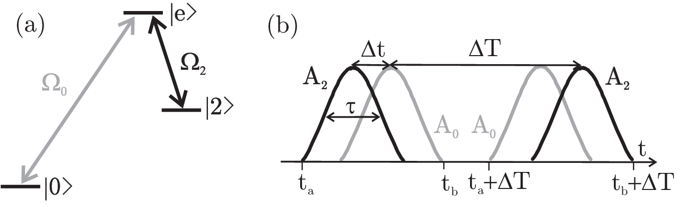
With all population initially in the $|0\rangle$-state and only $\Omega_{2}$ applied the system is in this dark state. Now, adiabatically increasing $\Omega_{0}$ and decreasing $\Omega_{2}$ causes population transfer from $|0\rangle$ to $|2\rangle$, while all population remains in $|D\rangle$ of Eq. (4). This implies that the excited state, $|e\rangle$ is never populated and hence no population is lost due to spontaneous emission.

STIRAP is well-suited for studying geometric phases, because no dynamic phase is acquired, $\omega^{D}=0$. The geometric phase is calculated by Eq. (3) with $\bar{R}=(\theta,\varphi_{2})$,

To obtain a non-zero $\gamma_{D}$, the phase difference between the two laser fields, $\varphi_{2}$, should be controlled and have a time-dependence with non-vanishing $\dot{\varphi}_{2}$. In order to be able to control the actual value of $\gamma_{D}$ we require that $\sin^{2}\theta=0$ before and after the pulse sequence, ensuring that only during the sequence a geometric phase is acquired. As stated in Eq. (4) $\sin^{2}\theta=|\Omega_{0}|^{2}/(|\Omega_{0}|^{2}+|\Omega_{2}|^{2})$, which implies that during one STIRAP process $\sin^{2}\theta$ is increased from zero to one. Applying a second STIRAP process, where $\Omega_{0}$ is decreased while $\Omega_{2}$ is increased, decreases $\sin^{2}\theta$ from one to zero. This second process transfers the population from $|2\rangle$ back to $|0\rangle$. The whole pulse sequence is shown in Fig. 1(b) and after this sequence the system ends up in

where $\gamma_{D}$ is calculated form Eq. (7) with $t_{i}=t_{a}$ and $t_{f}=t_{b}+\Delta T$ as defined in Fig. 1(b).

In the lambda system described above the geometric phase acquired by the dark state, $|D\rangle$ is a collective phase on the two atomic states, $|0\rangle$ and $|2\rangle$. We now turn to the tripod system shown in Fig. 2(a).

This system has the advantage that two dark states are populated and these acquire different geometric phases leading to relative phases between the atomic states as well as changes in their population due to changes in the interference of the two dark states. In the tripod system we can therefore calculate the geometric phase and see how it affects the measurable populations and relative phases between the atomic states. The tripod system further constitute a system, where a universal set of quantum gates can be implemented (see, e.g., Møller et al. 2007 and references therein). The level structure consists of three lower states ($|0\rangle$, $|1\rangle$ and $|2\rangle$) coupled to an excited state, $|e\rangle$, with three laser fields. These have Rabi frequencies $\Omega_{0}$, $\Omega_{1}$ and $\Omega_{2}$, respectively, and for simplicity we assume that they are all on resonance. We restrict ourselves to the case where the relative phase between $\Omega_{0}$ and $\Omega_{1}$, $\varphi_{01}$, is time-independent while the phase of $\Omega_{2}$, $\varphi_{2}(t)$, is time-dependent. The real amplitudes of all fields, $A_{0}(t)$, $A_{1}(t)$ and $A_{2}(t)$ are time-dependent and the Rabi frequencies explicitly read

The pulses are as in the lambda-system case modeled by the $\sin^{2}$-pulses in Eq. (6). When we apply the pulse sequence shown in Fig. 2(b), the STIRAP process transfers part of the population from $|0\rangle$ and $|1\rangle$ to $|2\rangle$ and back. During this process geometric phases are acquired. Calculations of the evolution of the system is presented in Sec. III for a closed system and in Sec. IV for an open system.

With the Lindblad operator $C_{0}=\sqrt{2\Gamma_{0}}|0\rangle\langle 0|$, $H^{\prime}=-i\hbar\Gamma_{0}|0\rangle\langle 0|$ and the non-Hermitian Hamiltonian of the tripod system, $\tilde{H}=H+H^{\prime}$ reads

In order to determine the time evolution of the system, we transform into the interaction picture with respect to $H^{\prime}$

The subscript $I$ indicates that the evolution is described in the interaction picture. This Hamiltonian is non-Hermitian due to the $\Gamma_{0}$-exponents and in order to determine the geometric phases we follow the procedure of Ref. Garrison and Wright 1988. We diagonalize $H_{I}$ and find the eigenvalues

and the right (subscript $r$) and left (subscript $l$) eigenvectors

The left and right eigenvectors fulfill the biorthonormal condition $\langle i_{l}|j_{r}\rangle_{I}=\delta_{i,j}$ Faisal 1987.

Initially $(t=t_{i})$ the eigenvectors of the open system [Eq. (42)] coincide with the eigenvectors of the closed system [Eq. (20)], and hence the initial state of the closed system is also the initial state of the open system

The adiabatic STIRAP evolution ensures that the system remains within the subspace spanned by $\{|D_{1r}(t)\rangle_{I},|D_{2r}(t)\rangle_{I}\}$. Inserting Eq. (43) into the time-dependent Schrödinger equation gives a set of equations that can be solved numerically for $C_{D_{1}}$ and $C_{D_{2}}$. Without loss of generality we write the solutions as

and expand the wave function as

The two dark states each acquire a complex geometric phase composed by real ($\gamma_{1}$ and $\gamma_{2}$) and imaginary parts ($\Gamma_{0}\alpha(t)$ and $\Gamma_{0}\beta(t)$) parameterized by the dephasing rate, $\Gamma_{0}$. As an example we choose an initial state $|\psi_{i}\rangle=|0\rangle$ and apply the pulse sequence in Fig. 2(b) with parameters leading to $\theta_{01}=\frac{\pi}{8}$, $\phi_{01}=\pi$ and $\gamma_{D_{1}}=-\pi$ (see details in caption of Fig. 3). As discussed in Sec. III this evolution corresponds to the Hadamard gate, Eq. (27) for the closed system. In Fig. 3 we show the evolution of the phases as a function of time for different values of the dephasing rate $\Gamma_{0}$. The real geometric phases $\gamma_{1}$ (light grey) and $\gamma_{2}$ (grey) are unaffected by the dephasing and their values are identical to the analytical result for the closed system [Eq. (24)], which are marked with crosses in Fig. 3. The exponents $\alpha$ and $\beta$ are also almost unaffected by the dephasing rate. The results for $\Gamma_{0}\tau=10^{-5}$ and $\Gamma_{0}\tau=10^{-3}$ (solid) are identical while increasing the dephasing to $\Gamma_{0}\tau=10^{-1}$ (dotted) gives only a small deviation. Experimentally dephasing rates can be kept below $\Gamma_{0}\tau=10^{-3}$ and for these values of $\Gamma_{0}$, $\alpha$ and $\beta$ are unaffected by the dephasing rate and hence the imaginary part of the phases $\Gamma_{0}\alpha$ and $\Gamma_{0}\beta$ scales linear with the dephasing rate. It should be noted that the value of $\alpha$ and $\beta$ depend on the initial state while $\gamma_{1}$ and $\gamma_{2}$ are unaffected and equal to the values in the closed system case.

Going back to the Schrödinger picture yields

where the wave function was re-normalized (factor $1/\sqrt{N}$) because the non-Hermitian Hamiltonian does not preserve the norm. In the $\{|0\rangle,|1\rangle\}$-basis an initial state in the Schrödinger picture $|\psi_{i}\rangle=a_{i}|0\rangle+b_{i}|1\rangle$ is transferred to a final non-normalized state $|\psi_{f}\rangle_{non-norm}=L|\psi_{i}\rangle=a_{f}|0\rangle+b_{f}|1\rangle$, with

The normalization constant, $N=|C_{D_{1}}(t_{i})|^{2}e^{-2\Gamma_{0}\alpha}+|C_{D_{2}}(t_{i})|^{2}e^{-2\Gamma_{0}\beta}$, depends on the initial state, and the final state reads $|\psi_{f}\rangle=\frac{1}{\sqrt{N}}|\psi_{f}\rangle_{non-norm}$. While the phases $\gamma_{1}$ and $\gamma_{2}$ are robust with respect to dephasing, the appearance of the imaginary phases, affects the population of the states.

Figure 4 shows the evolution of the population of the four states $(|0\rangle,|1\rangle,|e\rangle,|2\rangle)$ with initial state $|\psi_{i}\rangle=|0\rangle$ and the pulse sequence in Fig. 2(b) with parameters $\theta_{01}=\pi/8$, $\varphi_{01}=\pi$ and $\gamma_{D_{1}}=-\pi$ (see detailed parameters in the caption of Fig. 4). In the closed system these parameters lead to an implementation of the Hadamard gate and hence final populations $P_{0}=\frac{1}{2}$ and $P_{1}=\frac{1}{2}$. When we introduce dephasing $|\psi_{i}\rangle=|0\rangle$ leads to final population found from the no-jump evolution [Eq. (47)]

The deviation from the closed system case $(P_{0}=(\cos^{2}\theta_{01}-\sin^{2}\theta_{01})^{2},P_{1}=4\sin^{2}\theta_{01}\cos^{2}\theta_{01})$ is thus determined by the the two imaginary geometric phases, $\Gamma_{0}\alpha$ and $\Gamma_{0}\beta$. The values of $\alpha$ and $\beta$ are found by numerically solving the time-dependent Schrödinger equation. On the scale of Fig. 4 there is no deviation between the closed and the open system results for realistic dephasing rates.

For the present choice of parameters the system jumps in a small part of the Monte Carlo traces to the $|0\rangle$-state due to $C_{0}=\sqrt{2\Gamma_{0}}|0\rangle\langle 0|$. If a jump occurs at $t_{j}$ we expand the wave function ($|0\rangle$) in the adiabatic basis of the instantaneous eigenstates

After the jump the evolution is described by the no-jump non-Hermitian Hamiltonian [Eq. (IV.1)]. In the adiabatic basis we can describe this evolution by calculating the geometric and dynamic phases acquired by the four states. The dark part of the wave function evolves as described for the no-jump evolution. The bright eigenstates $(|+_{r}\rangle,|-_{r}\rangle)$ are separated energetically from each other and from the dark states, such that there is no diabatic population transfer among these. The bright states acquire a dynamic phase as well as a complex geometric phase that can be calculated directly Eq. (3). The complex geometric phase is the same for the two bright states