Finite-temperature Bell test for quasiparticle entanglement in the Fermi sea
Abstract
We demonstrate that the Bell test cannot be realized at finite temperatures in the vast majority of electronic setups proposed previously for quantum entanglement generation. This fundamental difficulty is shown to originate in a finite probability of quasiparticle emission from Fermi-sea detectors. In order to overcome the feedback problem we suggest a detection strategy, which takes advantage of a resonant coupling to the quasiparticle drains. Unlike other proposals the designed Bell test provides a possibility to determine the critical temperature for entanglement production in the solid state.
pacs
03.67.Mn, 05.30.Fk, 05.60.Gg, 73.23.-bIt is well-known that, unlike photons, quasiparticles in the Fermi sea injected from reservoirs, which are kept at thermal equilibrium, can be entangled by just a tunnel barrier.Bee03 This allows for particularly simple proposals for quantum quasiparticle entanglement, which do not involve interactions.Bee03; Bee04; Sam04a; Leb05; Lor05 Theoretical results for the entanglement production in different electronic setups have been summarized in Refs. Sam04b and Bee05a, while yet no experimental evidence of the quasiparticle entanglement in the Fermi sea has become available.
The quantum entanglement of two particles with respect to a spin-like degree of freedom can be accessed experimentally by measuring the spin correlator
| (1) |
where is the vector of Pauli matrices. The spin projection of the particles in the detectors and is measured with respect to the unit vectors and , correspondingly. If the correlation between the particles is of a classical origin the following Bell inequality holds,Cla69
| (2) |
for arbitrary choice of the unit vectors , , , . The violation of the inequality (2) is, therefore, sufficient but not necessary condition for quantum entanglement.
In solid-state electronics we deal with elementary excitations in the Fermi gas, which are referred to as quasiparticles. Even though the pairwise quasiparticle entanglementBur00; Bur03 is believed to be generated in many devices,Sam03; Sca04; Bee05b; Sam05 its experimental observation is obscured by the nature of electronic detectors. Those, unlike the photodetectors in optical setups, contain a number of quasiparticles in the ground state, which fill up available quantum levels below the Fermi energy. If a part of the device is at finite temperature the electron and hole excitations are spontaneously created near the Fermi surface resulting in a finite probability for a Fermi-sea detector to emit. Such processes are harmful for any sensible Bell test.
The problem of quasiparticle entanglement detection has been put forward in Refs. Kaw01 and Cht02, where the possibility to construct a Bell-type inequality with current cross-correlators is discussed. It has been suggested to take advantage of the generalized spin-correlator
| (3) |
where is a number of particles with a spin projection registered by the detector . (In solid state the role of spin can be played by other quantum degrees of freedom such as orbital momentum or isospin). Similarly to Eq. (1) the spin projection in Eq. (3) is measured with respect to the direction in the first detector and in the second one. Both definitions (1) and (3) are equivalent in the original Bell setup, if no more than two particles are received within the detection time and the detectors do not emit particles. In electronic circuits the number of quasiparticles is given by the time integral of a current flowing to the corresponding Fermi-sea reservoir
| (4) |
which is not restricted. For large detection times one typically observes , hence the Bell inequality (2) cannot be violated and the corresponding measurement is useless for entanglement detection. The difficulty has been discussed in Ref. Cht02 for zero temperature.
An essential problem occurs in the opposite limit , because defined by Eq. (4) can take on negative values. This leads to fluctuations with , which are explicitly forbidden in the Bell test. This situation is realized at finite temperatures. Then, the violation of Eq. (2) has no relation to the entanglement detection and the corresponding measurement is not of a Bell type.
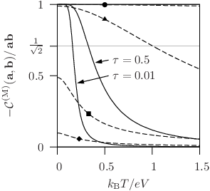
Thus, the violation of the inequality (2) with the correlator substituted by does not provide a conclusive evidence for quantum entanglement generation at any finite temperature. This difficulty clearly applies to the detection of electron-hole entanglementBee05a; Bee05b produced by tunneling events or by time-dependent gating. But even in more sophisticated setups where zero-temperature detectors and finite-temperature sources are represented by different metallic leads (in close resemblance to the original Bell proposal) the Bell test based on Eq. (3) is flawed. Examples include three-terminal fork geometriesLeb05 and four-terminal beam-splitter geometries with grounded detectors. We focus on the latter (see Fig. 1) due to a number of previously proposed realizations,Bee03; Sam04a; Leb05; Lor05; Sam03; Gio06; Fao07 which are mostly based on the directed transport along quantum-Hall edge channels. Minor modifications, such as lowering chemical potential in one of the detectors or increasing detection time, can suppress the probability of detector emission but lead, instead, to useless measurement with . The generic situation is illustrated in Fig. 2 for the case of electronic beam splitter.
For quantum particles the spin correlator from Eq. (3) is expressed through the expectation value
| (5) | |||
where and are regarded as operators. We introduce the function and the frequency-dependent cross-correlator
| (6) |
with . In Figs. 2,3 the correlator defined by experimentally measurable quantities (5,6) is compared with the exact result of the density matrix analysis of the final state.Bee05a
We restrict ourselves to an important class of systems which do not involve spin-dependent scattering, because the chances to generate quantum entanglement with respect to the spin degree of freedom are obviously maximized in such setups. The values of in Eq. (6) are related to the cross-correlator of the corresponding spin-independent problem as
| (7) | |||
| (8) |
This symmetry holds even for interacting electronic systems provided the absence of spin dephasing. It follows from Eqs. (7,8) that a neglection of the mean currentsLor05; Bee05a in Eq. (5) is equivalent to , hence the inequality (2) is violated with irrespective of voltages, temperature or other setup characteristics. Clearly, such violation has nothing to do with pairwise quantum entanglement. We will see that the problem persists even if the exact expression for is used.
In the absence of spin-dependent scattering the mean currents measured by the detectors do not depend on the directions and , . From Eqs. (5,6,7,8) we obtain
| (9) |
with a parameter given by the ratio
| (10) |
where both the cross-correlator and the product of the mean currents have to be calculated for the corresponding spin-independent problem.

An example of such a calculation can be performed within the Landauer-Büttiker scattering approach,Bla00 which is valid as far as inelastic processes in between the reservoirs can be disregarded. Within the scattering approach the mean current to the reservoir is given by
| (11) |
where is the Fermi distribution function, which depends on the temperature of the corresponding reservoir and the voltage bias applied. The frequency-dependent correlator (6) of the currents flowing to the reservoirs and reads,Bla00
| (12) |
| (13) |
Let us consider a generic beam splitter with no spin-dependent scattering depicted schematically in Fig. 1. Such a setup is characterized by an energy-independent -matrix
| (14) |
where unitary matrices and describe the transport from sources to detectors and from detectors to sources, correspondingly. We parameterize
| (15) |
where is the beam-splitter transparency and the spin index is omitted. Following the majority of proposals both detectors and the second source are grounded, i.e. , , while is the voltage applied between the sources.
At zero temperature the beam splitter actsBee05a as a source of spin-entangled Bell pairs
| (16) |
where the index refers to the detector number. Such an entanglement generation is due to the Pauli principle, which guarantees that a filled state with in the first source contains exactly two quasiparticles with the opposite spins.
The Bell pairs can be accessed at zero temperature by performing a time coincidence detection. For finite temperature in the sources the density matrix projection, which corresponds to a single particle in each detector, is derived in the Appendix ABee05a
| (17) |
where is the unit matrix in the two-particle Hilbert space and is an energy-independent weight factor
| (18) |
where is the Fermi distribution function in -th source. The result (17) describes the mixed Werner state,Wer89 which is entangled as far as according to the Wootters formula.Woo98 In the present case this condition is equivalent to with the critical temperature determined by the equationBee05a
| (19) |
From Eqs. (1,17) one obtains the exact spin correlator
| (20) |
which is plotted in Fig. 2 with the solid line for different values of the transparency parameter. The corresponding Bell inequality (2) can be violated for , which is, indeed, a sufficient condition for the entanglement. Whether or not such a Bell test can be performed by measuring current cross-correlator (3) is, however, an open question.
In order to answer this question we substitute the expression (14) for the -matrix to Eqs. (11,12), where the summation runs over the index . The correlator is, then, obtained from Eqs. (9,10) with , , and .
For we obtain
| (21) |
i.e. the corresponding measurement is useless for an entanglement detection. Indeed, such a long-time measurement is not projective, therefore it does not single out the state with one quasiparticle in each detector.Bay06
In the opposite limit we, however, find
| (22) |
hence the inequality (2) is violated for any temperature of the source. Thus, according to the density matrix analysis (17,20), the corresponding measurement is not of a Bell type. Both results (21) and (22) formally hold for any temperature of the detectors.
The transition from non Bell-type measurement to the useless measurement with the increase of is illustrated in Fig. 2. The Bell parameter defined with the correlator does not depend on the beam-splitter transparency and can easily exceed even in the absence of any entanglement.
The result of Eq. (22) is equivalent to
| (23) |
At the currents are sign-definite, hence Eq. (23) is exact for every single time-coincidence measurement in agreement with the prediction of the density matrix approach. For rising temperatures the correlation (23) holds only on average and is not sensitive to vanishing quantum entanglement in the final state of the beam splitter (17). Consequently, the inequality (2) with substituted by can be violated for arbitrarily high temperatures. The absence of critical temperature indicates once againFin05 that such a violation has nothing to do with the entanglement detection. Instead, the decay of with the temperature in Fig. 2 (dashed lines) is determined by the detection time .
Thus, the measurement of cannot be used for the entanglement test in the beam-splitter setup and the value of cannot be inferred from such a measurement as the matter of principle.
We propose a way to rescue the Bell measurement by coupling detectors via the energy filters, which are described by energy dependent scattering amplitudes: , where is the number of the detector. The use of energy-filters in the context of Bell measurement at zero temperature has been discussed in Ref. Les01. Let us illustrate our results for the case of identical filters with the Breit-Wigner form of the transmission amplitude
| (24) |
The -matrix of the full setup including the filters is given by
| (25) |
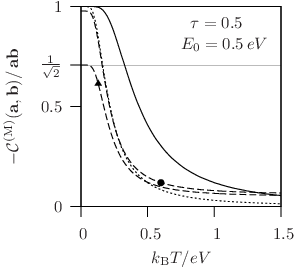
where , , etc. The condition for time-coincidence detection now reads . The currents can be made sign-definite by applying an additional voltage bias , as shown in Fig. 1. The current fluctuations due to temperature are not harmful for the Bell test as far as , which is the only restriction on the value of . In this case there is no requirement for an additional cooling of the detectors, so that a whole setup can be kept in temperature equilibrium. Moreover, for the dependence on vanishes, meaning that can be obtained experimentally from zero-frequency noise measurements. The feasibility of such a Bell test is illustrated in Fig. 3 for realistic values of the parameters.
For we obtain from Eqs. (9,10,12,24,25)
| (26) |
The result is plotted with the short-dashed line in Fig. 3. It is evident from the comparison with Eqs. (18,20) that the proposed measurement is always of the Bell type. The correlator (26) tends to the exact one (20) for . The setup efficiency is, however, exponentially low in this limit. The numerical results in the case of finite resonance width are plotted in Fig. 3 with the dashed lines. The test provides the lower estimate for the critical temperature.
In conclusion we point out the fundamental restrictions for the Bell test in electronic setups due to the quasiparticle emission from Fermi-sea detectors. We propose a way to rescue the Bell measurement by a resonant coupling to the detectors. We show that the lower estimate of the critical temperature for entanglement production can be experimentally obtained in the proposed setup.
This research was supported by the DFG Priority Programm 1285. The discussions with C. W. J. Beenakker, W. Belzig, and Yu. V. Nazarov are gratefully acknowledged.
Appendix A Density matrix projection
Following Ref. Bee05a we review the derivation of the density matrix projection (17) for final scattering state in the case of the setup depicted in Fig. 1. The density matrix of the incoming state is given by
| (27) |
where is the Fermi distribution function in the source , , and is the fermion annihilation operator for an incoming scattering state at the channel and energy . The annihilation operators for the outgoing scattering states, , are obtained from the relation,
| (28) |
where are the components of a unitary scattering matrix.
Thus, the density matrix of the final state is
| (29) |
where
| (30) |
In order to quantify the two-particle entanglement for the partition of Hilbert space with respect to the detectors, the state has to be projected onto the sectors of the Fock space with the energies and particle numbers in the corresponding detectors . The density matrix of the projection factorizes into a product state in all sectors except for the sector with and . Projection onto this sector is found from Eq. (29) as
| (31) | |||||
where is the unit matrix in the two-particle Hilbert space, is the Bell state (16), and the weight factor is determined from the condition as
| (32) |
From Eqs. (31,32) we obtain Eqs. (17,18). By substituting with , in Eq. (18) we can further simplify the parameter as
| (33) |
The critical temperature is determined from the equation , which is equivalent to Eq. (19).
Appendix B Evaluation of the correlator
B.1 Plain beam splitter
We evaluate the generalized spin-correlator given by Eqs. (9,10) in the framework of the scattering approach. By substituting the scattering matrix (14, 15), into Eq. (11) we calculate the mean currents, which are measured in the detectors , as
| (34) |
The cross-correlator (12) is found as
| (35) | |||||
The parameter given by Eq. (10) can be calculated analytically in two opposite limits:
B.2 Beam splitter with energy filters
We repeat the calculation in a more general case of an energy-dependent scattering matrix (25). From Eq. (11) we obtain the mean currents
| (38) | |||||
| (39) | |||||
where is the Fermi distribution function in the detectors. From Eq. (12) we calculate the cross-correlator
| (40) |
where the function is defined in Eq. (12). These expressions allow for the numerical evaluation of for arbitrary energy-dependent scattering matrix (25).
In the case of sharp resonances, such as those of the Breit-Wigner form (24) with , we have
| (41) |
and obtain from Eqs. (38,39,40,41)
| (42) |
where the Fermi functions are evaluated at the position of the resonance . For the value is exponentially small, hence Eq. (26) is justified. In general the setup is functional provided the detector voltage is sufficiently large to ensure that is much smaller than both and within the energy window of the filters.
References
- (1) C. W. J. Beenakker, C. Emary, M. Kindermann, and J. L. van Velsen, Phys. Rev. Lett. 91, 147901 (2003).
- (2) C. W. J. Beenakker and M. Kindermann, Phys. Rev. Lett. 92, 056801 (2004).
- (3) P. Samuelsson, E. V. Sukhorukov, and M. Büttiker, Phys. Rev. Lett. 92, 026805 (2004).
- (4) A. V. Lebedev, G. B. Lesovik, and G. Blatter, Phys. Rev. B 71, 045306 (2005).
- (5) A. Di Lorenzo and Y. V. Nazarov, Phys. Rev. Lett. 94, 210601 (2005).
- (6) P. Samuelsson, E. V. Sukhorukov, and M. Büttiker, Phys. Rev. B 70, 115330 (2004).
- (7) C. W. J. Beenakker, Proc. Int. School Phys. E. Fermi, Vol. 162 (IOS Press, Amsterdam, 2006).
- (8) J. F. Clauser, M. A. Horne, A. Shimony, and R. A. Holt, Phys. Rev. Lett. 23, 880 (1969).
- (9) G. Burkard, D. Loss, and E. V. Sukhorukov, Phys. Rev. B 61, R16303 (2000).
- (10) G. Burkard and D. Loss, Phys. Rev. Lett. 91, 087903 (2003).
- (11) P. Samuelsson, E. V. Sukhorukov, and M. Büttiker, Phys. Rev. Lett. 91, 157002 (2003).
- (12) V. Scarani, N. Gisin, and S. Popescu, Phys. Rev. Lett. 92, 167901 (2004).
- (13) C. W. J. Beenakker, M. Titov, and B. Trauzettel, Phys. Rev. Lett. 94, 186804 (2005).
- (14) P. Samuelsson and M. Büttiker, Phys. Rev. B 71, 245317 (2005).
- (15) S. Kawabata, J. Phys. Soc. Jpn. 70, 1210 (2001).
- (16) N. M. Chtchelkatchev, G. Blatter, G. B. Lesovik, and T. Martin, Phys. Rev. B 66, 161320(R) (2002).
- (17) V. Giovannetti, D. Frustaglia, F. Taddei, and R. Fazio, Phys. Rev. B 74, 115315 (2006); 75, 241305(R) (2007).
- (18) L. Faoro and F. Taddei, Phys. Rev. B 75, 165327 (2007).
- (19) Ya. M. Blanter and M. Büttiker, Phys. Rep. 336, 1 (2000).
- (20) R. F. Werner, Phys. Rev. A 40, 4277 (1989).
- (21) W. K. Wootters, Phys. Rev. Lett. 80, 2245 (1998).
- (22) K. V. Bayandin, G. B. Lesovik, and T. Martin, Phys. Rev. B 74, 085326 (2006).
- (23) B. V. Fine, F. Mintert, and A. Buchleitner, Phys. Rev. B 71, 153105 (2005).
- (24) G. B. Lesovik, T. Martin, and G. Blatter, Eur. Phys. J. B 24, 287 (2001).