MPP-2007-136
Holographic vector mesons from spectral functions
at finite baryon or isospin density
Abstract
We consider gauge/gravity duality with flavor for the finite-temperature field theory dual of the AdS-Schwarzschild black hole background with embedded D7-brane probes. In particular, we investigate spectral functions at finite baryon density in the black hole phase. We determine the resonance frequencies corresponding to meson-mass peaks as function of the quark mass over temperature ratio. We find that these frequencies have a minimum for a finite value of the quark mass. If the quotient of quark mass and temperature is increased further, the peaks move to larger frequencies. At the same time the peaks narrow, in agreement with the formation of nearly stable vector meson states which exactly reproduce the meson mass spectrum found at zero temperature. We also calculate the diffusion coefficient, which has finite value for all quark mass to temperature ratios, and exhibits a first-order phase transition. Finally we consider an isospin chemical potential and find that the spectral functions display a resonance peak splitting, similar to the isospin meson mass splitting observed in effective QCD models.
pacs
11.25.Tq, 11.25.Wx, 12.38.Mh, 11.10.WxI Introduction and Summary
Recently in the context of gauge/gravity duality, there has been an intensive study of the phase diagram of large supersymmetric Yang-Mills theory with added fundamental degrees of freedom, by considering the AdS-Schwarzschild black hole background with added D7-brane probes Babington:2003vm; Kirsch:2004km; Apreda:2005yz; Mateos:2006nu; Albash:2006ew; Hoyos:2006gb. There are two kinds of D7-brane probes in the black hole background: Either they end before reaching the black hole horizon, since the wrapped by the D7-brane probe shrinks to zero as in Karch:2002sh, or they reach all the way to the black hole horizon. The first class of embeddings is usually called ‘Minkowski embeddings’, while the second is referred to as ‘black hole embeddings’. The parameter which parametrizes different embeddings is the temperature normalized quark mass , which may be given in terms of the asymptotic value of the embedding coordinate at the AdS horizon. The phase transition between both classes of embeddings is of first order. The analysis of the meson spectrum shows that this phase transition corresponds to a fundamental confinement/deconfinement transition at which the mesons melt.
Particular interest has arisen in the more involved structure of the phase diagram when a baryon chemical potential is present Kobayashi:2006sb. It was argued that for non-vanishing baryon density, there are no embeddings of Minkowski type, and all embeddings reach the black hole horizon. This is due to the fact that a finite baryon density generates strings in the dual supergravity picture which pull the brane towards the black hole. A chemical potential for these baryons corresponds to a vev for the time component of the gauge field on the brane. In the dual thermal -gauge theory a baryon is composed of quarks, such that the baryon density can be directly translated into a quark density . The thermodynamic dual quantity of the quark density is the quark chemical potential . In the brane setup we use, the chemical potential is determined by the choice of quark density and by the embedding parameter .
Very recently, however, it was found that for a vanishing baryon number density, there may indeed be Minkowski embeddings if a constant vev is present, which does not depend on the holographic coordinate Karch:2007br; Mateos:2007vc; Nakamura:2006xk; Nakamura:2007nx; Ghoroku:2007re. The phase diagram found there is sketched in figure 1. In the grey shaded region, the baryon density vanishes () but temperature, quark mass and chemical potential can be nonzero. This low temperature region only supports Minkowski embeddings with the brane ending before reaching the horizon. In contrast, the unshaded region supports black hole embeddings with the branes ending on the black hole horizon. In this regime the baryon density does not vanish (). In this paper we exclusively explore the latter region. At the lower tip of the line separating from in figure 1, there exists also a small region of multivalued embeddings, which are thermodynamically unstable Mateos:2007vc.

In the black hole phase considered here, there is a fundamental phase transition between different black hole embeddings Kobayashi:2006sb. This is a first order transition, which occurs in a region of the phase diagram close to the separation line between the two regions with vanishing (gray shaded) and non-vanishing (unshaded) baryon density. This transition disappears above a critical value for the baryon density given by
| (1) |
In this paper we make use of the methods developed in the context of AdS/CFT applied to hydrodynamics, for instance Son:2002sd; Teaney:2006nc; Kovtun:2006pf, in order to determine the spectral function at finite temperature and finite baryon density. For vanishing chemical potential, a similar analysis of the spectral functions has been performed in Myers:2007we. It was found that the spectrum is discrete at large quark mass, or equivalently at low temperature. At low quark mass, a quasiparticle structure is seen which displays the broadening decay width of the mesons. As the mass decreases or temperature rises, the mesons are rendered unstable as the resonance frequencies develop imaginary parts. Modes corresponding to such frequencies are called quasinormal. These excitations are then dissipated in the plasma. – Note that for this case, there are also lattice gauge theory results Aarts:2007wj.
In this paper we study the differences in the spectral functions with and without chemical potential. Relating our work to the phase diagram shown in (Mateos:2007vc, figure 2) (and reproduced here in figure 1), we here consider the region of black hole embeddings (unshaded region) with nonvanishing quark density. We find that at low temperature to quark mass ratio, the spectrum is asymptotically discrete and coincides with the zero-temperature supersymmetric meson mass formula found in Kruczenski:2003be, which in our coordinates reads
| (2) |
In Kruczenski:2003be, denotes the asymptotic separation of the D3- and D7-branes and counts the nodes of the embedding fluctuations. Here we are considering s-wave modes in the Kaluza-Klein expansion of the D7 brane probe wrapping , so the angular quantum number is zero. We connect the structure of the spectra found to the phase diagram in figure 1: The meson mass behavior described above occurs close to the Minkowski region of the phase diagram, where temperature effects are subdominant. Moreover, as a function of decreasing temperature to quark mass ratio, the quasiparticle peaks behave differently with and without finite quark density. As discussed in Myers:2007we, at vanishing density the peak maxima move towards smaller frequencies as a function of increasing quark mass. Here, in the case of finite quark density, we observe a similar behavior at small quark mass. However, keeping the temperature fixed as we increase the quark mass further, the peaks turn around at a value and move to larger and larger frequencies as the associated mesons become more stable. Note that a turning point behavior was also observed for vanishing quark density in the context of quasinormal modes for scalar modes of melting mesons Hoyos:2006gb.
Our spectra also show that for given quark mass and temperature, lower meson excitations can be nearly stable in the plasma, while higher excitations remain unstable. At vanishing baryon density, the formation of resonance peaks for higher excitations has also been observed in Mateos:2007yp. We discuss the distinct behavior of resonance peaks in section III.2.2, including a comparison of the observed turning points at finite baryon density with previous results.
We also calculate the quark diffusion constant and show that at finite density, it exhibits the first-order fundamental phase transition up to the critical density given by . For very large values of the density, the diffusion constant asymptotes to . This reflects the fact that in this case, the free quarks outnumber the quarks bound in mesons.
As a second point we consider the case of an isospin chemical potential, on which previous work in the holographic context has appeared in Apreda:2005yz; Parnachev:2007bc. In this case, two coincident D7-brane probes are considered. In particular we extend the results of our previous paper Erdmenger:2007ap, in which we calculated the retarded Green function and diffusion coefficient at finite isospin chemical potential for the flat embedding . In this previous work we also restricted to the case of constant vev for the non-Abelian gauge field , where is the flavor and the Lorentz index. This means that we chose to be independent of the radial direction. In this case we found a non-analytic frequency dependence of the Green functions and the diffusion coefficient. Here we extend this work to the case of non-vanishing quark mass, leading to non-trivial D7 embeddings, and to the case of radially varying gauge field component . We find that spectral functions quantitatively deviate from the baryonic background case. Additionally, a splitting of quasi-particle resonances is observed, which depends on the magnitude of the chemical potential.
This paper is organized as follows. In the following section II, we introduce the gravity background, field and brane configuration, used for the subsequent calculations. We also sketch the method to obtain retarded real-time correlators of thermal field theories from supergravity calculations. In section III we discuss the spectral functions and diffusion behavior of fundamental matter at finite baryon density. For matter with isospin chemical potential, the same analysis is carried out in section IV. The results are briefly summarized in section V.
II Holographic setup and thermodynamics
II.1 Background and brane configuration
We consider asymptotically space-time which arises as the near horizon ††margin: test limit of a stack of coincident D3-branes. More precisely, our background is an black hole, which is the geometry dual to a field theory at finite temperature (see e.g. Policastro:2002se). We make use of the coordinates of Kobayashi:2006sb to write this background in Minkowski signature as
| (3) |
with the metric of the unit -sphere, where ††margin: test
| (4) |
Here is the radius, is the string coupling constant, the temperature, the number of colors. In the following some equations may be written more conviniently in terms of the dimensionless radial coordinate , which covers a range from at the event horizon to , representing the boundary of space.
Into this ten-dimensional space-time we embed coinciding D7-branes, hosting flavor gauge fields . The embedding we choose lets the D7-branes extend in all directions of space and, in the limit , wraps an on the . It is convenient to write the D7-brane action in coordinates where
| (5) |
with . From the viewpoint of ten dimensional Cartesian , is the angle between the subspace spanned by the 4,5,6,7-directions, into which the D7-branes extend perpendicular to the D3-branes, and the subspace spanned by the 8,9-directions, which are transverse to all branes.
Due to the symmetries of this background, the embeddings depend only on the radial coordinate . Defining , the embeddings of the D7-branes are parametrized by the functions . They describe the location of the D7-branes in -directions. Due to our choice of the gauge field fluctuations in the next subsection, the remaining three-sphere in this metric will not play a prominent role.
The metric induced on the D7-brane probe is then given by
| (6) |
Here and in what follows we use a prime to denote a derivative with respect to (resp. to in dimensionless equations). The symbol denotes the square root of the determinant of the induced metric on the D7-brane, which is given by
| (7) |
The table below gives an overview of the indices we use to refer to certain directions and subspaces.
![[Uncaptioned image]](0710.0334v3/tableCoords.png)
The background geometry described so far is dual to thermal supersymmetric Yang-Mills theory with additional hypermultiplets. These hypermultiplets arise from the lowest excitations of the strings stretching between the D7-branes and the background-generating D3-branes. The particles represented by the fundamental fields of the hypermultiplets model the quarks in our system. Their mass is given by the asymptotic value of the separation of the D3- and D7-branes. In the coordinates used here we write Myers:2007we
| (8) |
where we introduced the dimensionless scaled quark mass .
In addition to the parameters incorporated so far, we aim for a description of the system at finite chemical potential and baryon density . In field theory, a chemical potential is given by a nondynamical time component of the gauge field. In the gravity dual, this is obtained by introducing a -dependent gauge field component on the D7 brane probe. For now we consider a baryon chemical potential which is obtained from the subgroup of the flavor symmetry group. The sum over flavors then yields a factor of in front of the DBI action written down below.
The value of the chemical potential in the dual field theory is then given by
| (9) |
where we introduced the dimensionless quantity for convenience. We apply the same normalization to the gauge field and distinguish the dimensionful quantity from the dimensionless .
The action for the probe branes’ embedding function and gauge fields on the branes is
| (10) |
Here is the induced metric (6) on the brane, is the field strength tensor of the gauge fields on the brane and are the branes’ worldvolume coordinates. is the brane tension and the factor arises from the trace over the generators of the symmetry group under consideration. For finite baryon density, this factor will be different from that at finite isospin density.
In Kobayashi:2006sb, the dynamics of this system of branes and gauge fields was analyzed in view of describing phase transitions at finite baryon density. Here we use these results as a starting point which gives the background configuration of the brane embedding and the gauge field values at finite baryon density. To examine vector meson spectra, we will then investigate the dynamics of fluctuations in this gauge field background.
In the coordinates introduced above, the action for the embedding and the gauge fields’ field strength is obtained by inserting the induced metric and the field strength tensor into (10). As in Kobayashi:2006sb, we get
| (11) |
where is the field strength on the brane. depends solely on .
According to Kobayashi:2006sb, the equations of motion for the background fields are obtained after Legendre transforming the action (11). Varying this Legendre transformed action with respect to the field gives the equation of motion for the embeddings ,
| (12) | ||||
The dimensionless quantity is a constant of motion. It is related to the baryon number density by Kobayashi:2006sb
| (13) |
Below, equation (12) will be solved numerically for different initial values and . The boundary conditions used are
| (14) |
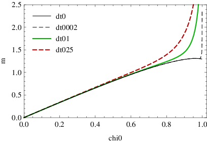
The quark mass is determined by . It is zero for and tends to infinity for . Figure 2 shows the dependence of the scaled quark mass on the starting value for different values of the baryon density parametrized by . In general, a small (large) is equivalent to a small (large) quark mass. For , can be viewed as being proportional to the large quark masses. At larger for vanishing , the quark mass reaches a finite value. In contrast, at finite baryon density, if is close to , the mass rapidly increases when increasing further. In embeddings with a phase transition, there exist more than one embedding for one specific mass value. In a small regime close to , there are more than one possible value of for a given . So in this small region, is not proportional to .
The equation of motion for the background gauge field is
| (15) |
Integrating both sides of the equation of motion from to some , and respecting the boundary condition Kobayashi:2006sb, we obtain the full background gauge field
| (16) |
Recall that the chemical potential of the field theory is given by and thus can be obtained from the formula above. Examples for the functional behavior of are shown in figure 3. Note that at a given baryon density there exists a minimal chemical potential which is reached in the limit of massles quarks.
The asymptotic form of the fields and can be found from the equations of motion in the boundary limit ,
| (17) | ||||
| (18) |
Here is the chemical potential, is the dimensionless quark mass parameter given in (8), is related to the quark condensate (but irrelevant in this work) and is related to the baryon number density as stated in (13). See also figure 3 for this asymptotic behavior. The -coordinate runs from the horizon value to the boundary at . In most of this range, the gauge field is almost constant and reaches its asymptotic value, the chemical potential , at . Only near the horizon the field drops rapidly to zero. For small , the curves asymptote to the lowest (red) curve. So there is a minimal chemical potential for fixed baryon density in this setup. At small baryon density () the embeddings resemble the Minkowski and black hole embeddings known from the case without a chemical potential. Only a thin spike always reaches down to the horizon.
In the setup described in this section we restrict ourselves to the regime of so called ‘black hole embeddings’ which are those embeddings ending on the horizon of the black hole, opposed to ‘Minkowski embeddings’ , which would reach without touching the horizon. The black hole embeddings we use for this work (see figure 3) are not capable of describing matter in all possible phases. In fact we are able to cover the regime of fixed and thus examine thermal systems in the canonical ensemble at finite baryon density. For a detailed discussion of this aspect see Karch:2007br; Mateos:2007vc.


II.2 Holographic spectral functions
Spectral functions contain information about the quasiparticle spectrum of a given theory. Recently, methods were developed to compute spectral functions from the holographic duals of strongly coupled finite temperature gauge theories. In this work we extend these results to investigate the quasiparticle spectrum corresponding to vector mesons in the limit of vanishing spatial momentum. Therefore, we analyze the holographic dual to spectral functions for thermal supersymmetric Yang-Mills theory with fundamental degrees of freedom (quarks) at finite baryon density and finite chemical potential. We compute the spectral densities for the flavor current , which is dual to the fluctuations of the flavor gauge field on the supergravity side.
Within field theory, the spectral function of some operator is defined via the imaginary part of the retarded Green function as follows
| (19) |
where Energy and spatial momentum may be written in a four vector and the Green function may be written as
| (20) |
One may find singularities of in the lower half of the complex -plane, including hydrodynamic poles of the retarded real-time Green function. Consider for example
| (21) |
These poles emerge as peaks in the spectral densities,
| (22) |
located at with a width given by . These peaks are interpreted as quasi-particles if their lifetime is considerably long, i.e. if .
In this paper we use the gauge/gravity duality prescription of Son:2002sd for calculating Green functions in Minkowski space-time. For further reference, we outline this prescription briefly in the subsequent. Starting out from a classical supergravity action for the gauge field , according to Son:2002sd we extract the function (containing metric factors and the metric determinant) in front of the kinetic term ,
| (23) |
Then we perform a Fourier transformation and solve the linearized equations of motion for the fields in momentum space. The solutions in general are functions of all five coordinates in Anti-de Sitter space. Near the boundary we may separate the radial behavior from the boundary dynamics by writing
| (24) |
where is the value of the supergravity field at the boundary of depending only on the four flat boundary coordinates. Thus by definition we have . Then the retarded thermal Green function is given by
| (25) |
The thermal correlators obtained in this way display hydrodynamic properties, such as poles located at complex frequencies. They are used to compute the spectral densities (19). We are going to compute the functions numerically in the limit of vanishing spatial momentum . The functions are then obtained by dividing out the boundary value . Numerically we obtain the boundary value by computing the solution at a fixed large .
III Spectral functions at finite baryon density
III.1 Baryon diffusion
In this section we calculate the baryon diffusion coefficient and its dependence on the baryon density. As discussed in Mateos:2007vc, the baryon density affects the location and the presence of the fundamental phase transition between two black hole embeddings observed in Kobayashi:2006sb. This first order transition is present only very close to the separation line between the regions of zero and non-zero baryon density shown in figure 1.
We show that this fundamental phase transition may also be seen in the diffusion coefficient for quark diffusion. In order to compute the diffusion using holography, we use the membrane paradigm approach developed in Kovtun:2003wp and extended in Myers:2007we. This method allows to compute various transport coefficients in Dp/Dq-brane setups from the metric coefficients. The resulting formula for our background is the same as in Myers:2007we,
| (26) |


The dependence of on the baryon density and on the quark mass originates from the dependence of the embedding on these variables. The results for are shown in figure 4. The thick solid line shows the diffusion constant at vanishing baryon density found in in Myers:2007we, which reaches at the fundamental phase transition. Increasing the baryon density, the diffusion coefficient curve is lifted up for small temperatures, still showing a phase transition up to the critical density . This is the same value as found in Kobayashi:2006sb in the context of the phase transition of the quark condensate.
The diffusion coefficient never vanishes for finite density. Both in the limit of and , converges to for all densities, i.e. to the same value as for vanishing baryon density, as given for instance in Kovtun:2003wp for R-charge diffusion. At the phase transition, the diffusion constant develops a nonzero minimum at finite baryon density. Furthermore, the location of the first order phase transition moves to lower values of while we increase towards its critical value.
In order to give a physical explanation for this behavior, we focus on the case without baryon density first. We see that the diffusion coefficient vanishes at the temperature of the fundamental deconfinement transition. This is simply due to the fact that at and below this temperature, all charge carriers are bound into mesons not carrying any baryon number.
For non-zero baryon density however, there is a fixed number of charge carriers (free quarks) present at any finite temperature. This implies that the diffusion coefficient never vanishes. Switching on a very small baryon density, even below the phase transition, where most of the quarks are bound into mesons, by definition there will still be a finite amount of free quarks. By increasing the baryon density, we increase the amount free quarks, which at some point outnumber the quarks bound in mesons. Therefore in the large density limit the diffusion coefficient approaches for all values of , because only a negligible fraction of the quarks is still bound in this limit.
Note that as discussed in Karch:2007br; Kobayashi:2006sb; Mateos:2007vc there exists a region in the phase diagram at small and where the embeddings are unstable. In figure 4, this corresponds to the region just below the phase transition at small baryon density. This instability disappears for large .
III.2 Vector mesons in the black hole phase
III.2.1 Application of calculation method
We now compute the spectral functions of flavor currents at finite baryon density , chemical potential and temperature in the ‘black hole phase’. As black hole phase the authors of Karch:2007br denote the phase of matter which has nonzero baryon density. Compared to the limit of vanishing chemical potential treated in Myers:2007we, we discover a qualitatively different behavior of the finite temperature oscillations corresponding to vector meson resonances.
To obtain the spectral functions, we compute the correlations of flavor gauge field fluctuations about the background given by (11), denoting the full gauge field by
| (27) |
According to section II.1, the background field has a non-vanishing time component, which depends solely on . The fluctuations in turn are gauged to have non-vanishing components along the Minkowski coordinates only and only depend on these coordinates and on . Additionally they are assumed to be small, so that it suffices to consider their linearized equations of motion. At this point we neglect the fluctuation of the scalar and pseudoscalar modes and their coupling to the vector fluctuations. In fact there is no such coupling in the limit of vanishing spatial momentum, which we restrict to below.
The resulting equations of motion are obtained from the action (10), where we introduce small fluctuations by setting with . The background gauge field is given by (15). The fluctuations now propagate on a background given by
| (28) |
and their dynamics is determined by the Lagrangian
| (29) |
with the fluctuation field strength . Since the fluctuations and their derivatives are chosen to be small, we consider their equations of motion only up to linear order, as derived from the part of the Lagrangian which is quadratic in the fields and their derivatives. Denoting this part by , we get
| (30) |
Here and below we use upper indices on to denote elements of . The equations of motion for the components of are
| (31) |
The terms of the corresponding on-shell action at the -boundaries are (with as an index for the coordinate , not summed)
| (32) |
Note that on the boundary at , the background matrix reduces to the induced D7-brane metric . Therefore, the analytic expression for boundary contributions to the on-shell action is identical to the one found in Myers:2007we. There, the coordinates in Minkowski directions were chosen such that the fluctuation four vector exhibits only one non vanishing spatial component, e. g. in -direction as . Then the action was expressed in terms of the gauge invariant field component combinations
| (33) |
In the case of vanishing spatial momentum , the Green functions for the different components coincide and were computed as Myers:2007we
| (34) |
where the in the denominator divides out the boundary value of the field in the limit of large , as discussed after (25). The indices on the Green function denote the components of the operators in the correlation function, in our case all off-diagonal correlations (as , for example) vanish.
In our case of finite baryon density, new features arise through the modified embedding and gauge field background, which enter the equations of motion (31) for the field fluctuations. To apply the prescription to calculate the Green function, we Fourier transform the fields as
| (35) |
As above, we are free to choose our coordinate system to give us a momentum vector of the fluctuation with nonvanishing spatial momentum only in -direction, .
For simplicity we restrict ourselves to vanishing spatial momentum . In this case the equations of motion for transversal fluctuations match those for longitudinal fluctuations . For a more detailed discussion see Myers:2007we. As an example consider the equation of motion obtained from (31) with , determining ,
| (36) |
The symbol denotes the dimensionless frequency , and we made use of the dimensionless radial coordinate .
In order to numerically integrate this equation, we determine local solutions of that equation near the horizon . These can be used to compute initial values in order to integrate (36) forward towards the boundary. The equation of motion (36) has coefficients which are singular at the horizon. According to standard methods Bender, the local solution of this equation behaves as , where is a so-called ‘index’ of the differential equation. We compute the possible indices to be
| (37) |
Only the negative one will be retained in the following, since it casts the solutions into the physically relevant incoming waves at the horizon and therefore satisfies the incoming wave boundary condition. The solution can be split into two factors, which are and some function , which is regular at the horizon. The first coefficients of a series expansion of can be found recursively as described in Teaney:2006nc; Kovtun:2006pf. At the horizon the local solution then reads
| (38) | ||||
So, asymptotically assumes values
| (39) |
For the calculation of numbers, we have to specify the baryon density and the mass parameter to obtain the embeddings used in (36). Then we obtain a solution for a given frequency using initial values (38) and (39) in the equation of motion (36). This eventually gives us the numerical solutions for .
III.2.2 Results for spectral functions
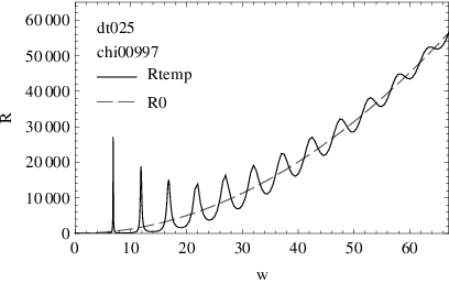
We now discuss the resulting spectral functions at finite baryon density, and observe crucial qualitative differences compared to the case of vanishing baryon density. In figures 5 to 8, some examples for the spectral function at fixed baryon density are shown. To emphasize the resonance peaks, in some plots we subtract the quantity
| (41) |
around which the spectral functions oscillate, cf. figure 9.
The graphs are obtained for a value of above (given by (1)), where the fundamental phase transition does not occur. The different curves in these plots show the spectral functions for different quark masses, corresponding to different positions on the solid blue line in the phase diagram shown in figure 1. Regardless whether we chose to be below or above the critical value of , we observe the following behavior of the spectral functions with respect to changes in the quark mass to temperature ratio.
Increasing the quark mass from zero to small finite values results in more and more pronounced peaks of the spectral functions. This eventually leads to the formation of resonance peaks in the spectrum. At small masses, though, there are no narrow peaks. Only some maxima in the spectral functions are visible. At the same time as these maxima evolve into resonances with increasing quark mass, their position changes and moves to lower freqencies , see figure 5. This behavior was also observed for the case of vanishing baryon density in Myers:2007we.
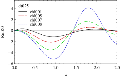
However, further increasing the quark mass leads to a crucial difference to the case of vanishing baryon density. Above a value of the quark mass, parametrized by , the peaks change their direction of motion and move to larger values of , see figure 6. Still the maxima evolve into more and more distinct peaks.
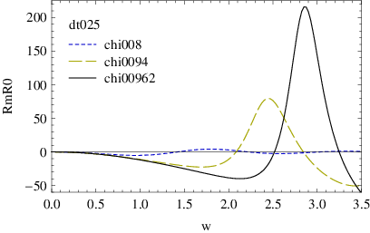
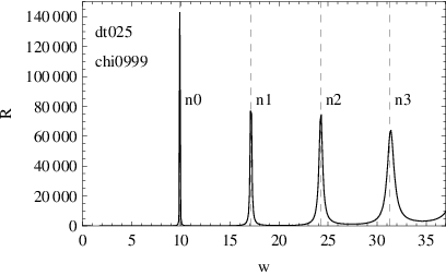
Eventually at very large quark masses, given by closer and closer to 1, the positions of the peaks asymptotically reach exactly those frequencies which correspond to the masses of the vector mesons at zero temperature Kruczenski:2003be. In our coordinates, these masses are given by
| (42) |
where labels the Kaluza-Klein modes arising from the D7-brane wrapping , and is the radial distance in -direction between the stack of D3-branes and the D7, evaluated at the -boundary,
| (43) |
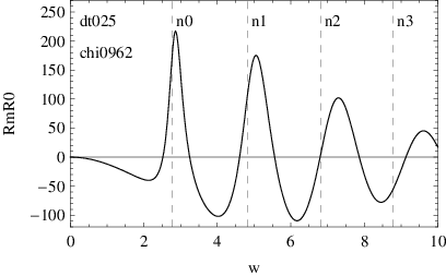
The formation of a line-like spectrum can be interpreted as the evolution of highly unstable quasi-particle excitations in the plasma into quark bound states, finally turning into nearly stable vector mesons, cf. figures 7 and 8.
We now consider the turning behavior of the resonance peaks shown in figures 5 and 6. There are two different scenarios, depending on whether the quark mass is small or large.
First, when the quark mass is very small , we are in the regime of the phase diagram corresponding to the right half of figure 1. In this regime the influence of the Minkowski phase is negligible, as we are deeply inside the black hole phase. We therefore observe only broad structures in the spectral functions, instead of peaks.
Second, when the quark mass is very large, , or equivalently the temperature is very small, the quarks behave just as they would at zero temperature, forming a line-like spectrum. This regime corresponds to the left side of the phase diagram in figure 1, where all curves of constant asymptote to the Minkowski phase.
The turning of the resonance peaks is associated to being in the first or in the second regime. At the two regimes are connected and none of them is dominant.
The turning behavior is best understood by following a line of constant density in the phase diagram of figure 1. Consider for instance the solid blue line in figure 1, starting at large temperatures/small masses on the right of the plot. First, we are deep in the unshaded region (), far inside the black hole phase. Moving along to lower , the solid blue line in figure 1 rapidly bends upwards, and asymptotes to both the line corresponding to the onset of the fundamental phase transition, as well as to the separation line between black hole and Minkowski phase (gray region).
This may be interpreted as the quarks joining in bound states. Increasing the mass further, quarks form almost stable mesons, which give rise to resonance peaks at larger frequency if the quark mass is increased. The confined and deconfined phase are coexistent asymptotically for .
We also observe a dependence of on the baryon density. As the baryon density is increased from zero, the value of decreases.
Figures 8 and 9 show that higher excitations from the Kaluza-Klein tower are less stable. While the first resonance peaks in this plot are very narrow, the following peaks show a broadening with decreasing amplitude.
This broadening of the resonances is due to the behaviour of the quasinormal modes of the fluctuations, which correspond to the poles of the correlators in the complex plane, as described in the example (21) and sketched in figure 10. The location of the resonance peaks on the real frequency axis corresponds to the real part of the quasinormal modes. It is a known fact that the the quasinormal modes develop a larger real and imaginary part at higher . So the sharp resonances at low , which correspond to quasiparticles of long lifetime, originate from poles whith small imaginary part. For higher excitations in at larger , the resonances broaden and get damped due to larger imaginary parts of the corresponding quasi normal modes.


For increasing mass we described above that the peaks of the spectral functions first move to smaller frequencies until they reach the turning point . Further increasing the mass leads to the peaks moving to larger frequencies, asymptotically approaching the line spectrum. This behavior can be translated into a movement of the quasinormal modes in the complex plane. It would be interesting to compare our results to a direct calculation of the quasinormal modes of vector fluctuations in analogy to Hoyos:2006gb.
In Hoyos:2006gb the quasinormal modes are considered for scalar fluctuations exclusively, at vanishing baryon density. The authors observe that starting from the massless case, the real part of the quasinormal frequencies increases with the quark mass first, and then turns around to decrease. This behavior agrees with the peak movement for scalar spectral functions observed in (Myers:2007we, figure 9) (above the fundamental phase transition, ) where the scalar meson resonances move to higher frequency first, turn around and move to smaller frequency increasing the mass further. These results do not contradict the present work since we consider vector modes exclusively. The vector meson spectra considered in Myers:2007we at vanishing baryon density only show peaks moving to smaller frequency as the quark mass is increased. Note that the authors there continue to consider black hole embeddings below the fundamental phase transition which are only metastable, the Minkowski embeddings being thermodynamically favored. At small baryon density and small quark mass our spectra are virtually coincident with those of Myers:2007we. In our case, at finite baryon density, black hole embeddings are favored for all values of the mass over temperature ratio. At small values of in the phase diagram of figure 1, we are very close to the Minkowski regime, temperature effects are small, and the meson mass is proportional to the quark mass as in the supersymmetric case. Therefore, the peaks in the spectral function move to the right (higher frequencies) as function of increasing quark mass.
The turning point in the location of the peaks is a consequence of the transition between two regimes, i.e. the temperature-dominated one also observed in Myers:2007we, and the potential-dominated one which asymptotes to the supersymmetric spectrum.
We expect the physical interpretation of the left-moving of the peaks in the temperature-dominated regime to be related to the strong dissipative effects present in this case. This is consistent with the large baryon diffusion coefficient present in this regime as discussed in section III.1 and shown in figure 4. A detailed understanding of the physical picture in this regime requires a quantitative study of the quasipaticle behavior which we leave to future work.
In our approach it is straightforward to investigate the limit since black hole embeddings are thermodynamically favored even near at finite baryon density. We expect that a right-moving of the peaks consistent with the SUSY spectrum should also be observable for Minkowski embeddings at vanishing baryon density. However this has not been investigated for vector modes neither in Hoyos:2006gb nor in Myers:2007we.
IV Spectral functions at finite isospin density
IV.1 Radially varying -background gauge field
In order to examine the case in the strongly coupled plasma, we extend our previous analysis of vector meson spectral functions to a chemical potential with -flavor (isospin) structure. Starting from the general action
| (44) |
we now consider field strength tensors
| (45) |
with the Pauli matrices and given by equation (27). The factor is due to the introduction of dimensionless fields as described below (9). In order to obtain a finite isospin-charge density and its conjugate chemical potential , we introduce an -background gauge field Erdmenger:2007ap
| (46) |
This specific choice of the 3-direction in flavor space as well as spacetime dependence simplifies the isospin background field strength, such that we get two copies of the baryonic background on the diagonal of the flavor matrix,
| (47) |
The action for the isospin background differs from the action (11) for the baryonic background only by a group theoretical factor: The factor (compare (44)) replaces the baryonic factor in equation (10), which arises by summation over the representations. We can thus use the embeddings and background field solutions of the baryonic case of Kobayashi:2006sb, listed here in section II.1. As before, we collect the induced metric and the background field strength in the background tensor .
We apply the background field method in analogy to the baryonic case examined in section III. As before, we obtain the quadratic action by expanding the determinant and square root in fluctuations . The term linear in fluctuations again vanishes by the equation of motion for our background field. This leaves the quadratic action
| (48) |
Note that besides the familiar Maxwell term, two other terms appear, which are due to the non-Abelian structure. One of the new terms depends linearly, the other quadratically on the background gauge field and both contribute nontrivially to the dynamics. The equation of motion for gauge field fluctuations on the D7-brane is
| (49) | ||||
with the modified field strength linear in fluctuations .
Integration by parts of (48) and application of (49) yields the on-shell action
| (50) |
The three flavor field equations of motion (flavor index ) for fluctuations in transversal Lorentz-directions can again be written in terms of the combination . At vanishing spatial momentum we get
| (51) | ||||
| (52) | ||||
| (53) |
Note that we use the dimensionless background gauge field and . Despite the presence of the new non-Abelian terms, at vanishing spatial momentum the equations of motion for longitudinal fluctuations are the same as the transversal equations (51), (52) and (53), such that .
Note at this point that there are two essential differences which distinguish this setup from the approach with a constant potential at vanishing mass followed in Erdmenger:2007ap. First, the inverse metric coefficients contain the embedding function computed with varying background gauge field. Second, the background gauge field giving rise to the chemical potential now depends on .
Two of the ordinary second order differential equations (51), (52), (53) are coupled through their flavor structure. Decoupling can be achieved by transformation to the flavor combinations Erdmenger:2007ap
| (54) |
The equations of motion for these fields are given by
| (55) | ||||
| (56) | ||||
| (57) |
with dimensionless and . Proceeding as described in section III, we determine the local solution of (55), (56) and (57) at the horizon. The indices turn out to be
| (58) |
Since in the setup considered here, we are left with the same index as in (37) for the baryon case. Therefore, here the chemical potential does not influence the singular behavior of the fluctuations at the horizon. The local solution coincides to linear order with the baryonic solution given in (38).
Application of the recipe described in section II.2 yields the spectral functions of flavor current correlators shown in figures 11 and 12. Note that after transforming to flavor combinations and , given in (54), the diagonal elements of the propagation submatrix in flavor-transverse directions vanish, , while the off-diagonal elements give non-vanishing contributions. However, the component , longitudinal in flavor space, is not influenced by the isospin chemical potential, such that is nonzero, while other combinations with vanish (see Erdmenger:2007ap for details).
Introducing the chemical potential as described above for a zero-temperature background, we obtain the gauge field correlators in analogy to Freedman:1998tz. The resulting spectral function for the field theory at zero temperature but finite chemical potential and density is given by
| (59) |
with the dimensionless chemical potential . Note that (59) is independent of the temperature. This part is always subtracted when we consider spectral functions at finite temperature, in order to determine the effect of finite temperature separately, as we did in the baryonic case.
IV.2 Results at finite isospin density
In figure 11 we compare typical spectral functions found for the isospin case (solid lines) with that found in the baryonic case (dashed line). While the qualitative behavior of the isospin spectral functions agrees with the one of the baryonic spectral functions, there nevertheless is a quantitative difference for the components , which are transversal to the background in flavor space. We find that the propagator for flavor combinations exhibits a spectral function for which the zeroes as well as the peaks are shifted to higher frequencies, compared to the Abelian case curve. For the spectral function computed from , the opposite is true. Its zeroes and peaks appear at lower frequencies. As seen from figure 12, also the quasiparticle resonances of these two different flavor correlations show distinct behavior. The quasiparticle resonance peak in the spectral function appears at higher frequencies than expected from the vector meson mass formula (2) (shown as dashed grey vertical lines in figure 12). The other flavor-transversal spectral function displays a resonance at lower frequency than observed in the baryonic curve. The spectral function for the third flavor direction behaves as in the baryonic case.


This may be viewed as a splitting of the resonance peak into three distinct peaks with equal amplitudes. This is due to the fact that we explicitly break the symmetry in flavor space by our choice of the background field . Decreasing the chemical potential reduces the distance of the two outer resonance peaks from the one in the middle and therefore the splitting is reduced.
The described behavior resembles the mass splitting of mesons in presence of a isospin chemical potential expected to occur in QCD He:2005nk; Chang:2007sr. A linear dependence of the separation of the peaks on the chemical potential is expected. Our observations confirm this behavior. Since our vector mesons are isospin triplets and we break the isospin symmetry explicitly, we see that in this respect our model is in qualitative agreement with effective QCD models. Note also the complementary discussion of this point in Aharony:2007uu.
To conclude this section, we comment on the relation of the present results to those of our previous paper Erdmenger:2007ap where we considered a constant non-Abelian gauge field background for zero quark mass. From equation (58), the difference between a constant non-vanishing background gauge field and the varying one becomes clear. In Erdmenger:2007ap the field is chosen to be constant in and terms quadratic in the background gauge field are neglected. This implies that the square in (55) and (56) is replaced by , such that we obtain the indices instead of (58). If we additionally assume , then the under the square root can be neglected. In this case the spectral function develops a non-analytic structure coming from the factor in the index.
However in the case considered here, the background gauge field is a non-constant function of which vanishes at the horizon. Therefore the indices have the usual form from (58), and there is no non-analytic behavior of the spectral functions, at least none originating from the indices.
It will also be interesting to consider isospin diffusion in the setup of the present paper. However, in order to see non-Abelian effects in the diffusion coefficient, we need to give the background gauge field a more general direction in flavor space or a dependence on further space-time coordinates besides . In that case, we will have a non-Abelian term in the background field strength in contrast to considered here.
V Conclusion
Two distinct setups were examined here at non-zero charge density in the black hole phase. First, switching on a baryon chemical potential at non-zero baryon density, we find that nearly stable vector mesons exist close to the transition line to the Minkowski phase. Far from this line, at small quark masses, we essentially recover the picture given in the case of vanishing chemical potential Myers:2007we. Increasing the quark mass beyond a distinct value, the plasma changes its behavior in order to asymptotically behave as it would at zero temperature. In the spectral functions we computed, this zero-temperature-like behavior is found in form of line-like resonances, exactly reproducing the zero-temperature supersymmetric vector meson mass spectrum. A turning point at , where , is observed: Below , the resonance peaks move to lower frequencies as function of rising quark mass. This behavior of the system resembles the behavior known of that system without a chemical potential Myers:2007we. Above , the resonance peaks move to higher frequencies as function of the quark mass. This is the zero-temperature-like regime. Moreover, an examination of the diffusion coefficient reveals that the phase transition separating two different black hole phases Kobayashi:2006sb is shifted towards smaller temperature as the baryon density is increased.
Second, we switched on a nonzero isospin density, and equivalently an isospin chemical potential arises. The spectral functions in this case show a qualitatively similar behavior as those for baryonic potential. However, we additionally observe a splitting of the single resonance peak at vanishing isospin potential into three distinct resonances. This suggests that by explicitly breaking the flavor symmetry by a chemical potential, the isospin triplet states, vector mesons in our case, show a mass splitting similar to that observed for QCD He:2005nk. It is an interesting task to explore the features of this isospin theory in greater detail in order to compare with available lattice data and effective QCD models Kogut:2002zg; Kogut:2002tm; Kogut:2004zg; Splittorff:2000mm; Loewe:2002tw; Barducci:2004tt; Sannino:2002wp; Ebert:2005cs; Ebert:2005wr. In most of these approaches, baryon and isospin chemical potential are considered at the same time, which suggests another promising extension of this work. Moreover, in the context of gravity duals, it will be interesting to compare our results for the isospin chemical potential to the recent work Aharony:2007uu.
Alternatively, instead of giving the gauge field time component a non-vanishing vev, one may also switch on B-field components and connect the framework developed in Erdmenger:2007bn; Albash:2007bk; Albash:2007bq with the calculation of spectral functions for the dual gauge theory.
Acknowledgements.
We are grateful to P. Kerner, C. Greubel, K. Landsteiner, D. Mateos, G. Policastro, A. Starinets, L. Yaffe and M. Zagermann for useful discussions and correspondence, as well as to R. Myers for suggesting to consider a -dependent component in the isospin case. Part of this work was funded by the Cluster of Excellence for Fundamental Physics – Origin and Structure of the Universe.Appendix A Notation
The five-dimensional Schwarzschild black hole space in which we work is endowed with a metric of signature , as given explicitly in (3). We make use of the Einstein notation to indicate sums over Lorentz indices, and additionally simply sum over non-Lorentz indices, such as gauge group indices, whenever they occur twice in a term.
To distinguish between vectors in different dimensions of the space, we use bold symbols like for vectors in the the three spatial dimensions which do not live along the radial coordinate. Four-vectors which do not have components along the radial coordinates are denoted by symbols with an arrow on top, as .
The Green functions considered give correlations between currents and . These currents couple to fields and respectively. In our notation we use symbols such as to denote correlators of currents coupling to fields and , with flavor indices and Lorentz indices . If no other indices are of relevance for the discussion we restrict ourselves to Lorentz indices. For the gauge field combinations and given in (54), we obtain Green functions or denoting correlators of the corresponding currents.
References
- (1) J. Babington, J. Erdmenger, N. J. Evans, Z. Guralnik, and I. Kirsch, Chiral symmetry breaking and pions in non-supersymmetric gauge / gravity duals, Phys. Rev. D69 (2004) 066007, hep-th/0306018.
- (2) I. Kirsch, Generalizations of the AdS/CFT correspondence, Fortsch. Phys. 52 (2004) 727–826, hep-th/0406274.
- (3) R. Apreda, J. Erdmenger, N. Evans, and Z. Guralnik, Strong coupling effective Higgs potential and a first order thermal phase transition from AdS/CFT duality, Phys. Rev. D71 (2005) 126002, hep-th/0504151.
- (4) D. Mateos, R. C. Myers, and R. M. Thomson, Holographic phase transitions with fundamental matter, Phys. Rev. Lett. 97 (2006) 091601, hep-th/0605046.
- (5) T. Albash, V. Filev, C. V. Johnson, and A. Kundu, A topology-changing phase transition and the dynamics of flavour, hep-th/0605088.
- (6) C. Hoyos-Badajoz, K. Landsteiner, and S. Montero, Holographic Meson Melting, JHEP 04 (2007) 031, hep-th/0612169.
- (7) A. Karch and E. Katz, Adding flavor to AdS/CFT, JHEP 06 (2002) 043, hep-th/0205236.
- (8) S. Kobayashi, D. Mateos, S. Matsuura, R. C. Myers, and R. M. Thomson, Holographic phase transitions at finite baryon density, JHEP 02 (2007) 016, hep-th/0611099.
- (9) A. Karch and A. O’Bannon, Holographic Thermodynamics at Finite Baryon Density: Some Exact Results, JHEP 11 (2007) 074, arXiv:0709.0570 [hep-th].
- (10) D. Mateos, S. Matsuura, R. C. Myers, and R. M. Thomson, Holographic phase transitions at finite chemical potential, JHEP 11 (2007) 085, arXiv:0709.1225 [hep-th].
- (11) S. Nakamura, Y. Seo, S.-J. Sin, and K. P. Yogendran, A new phase at finite quark density from AdS/CFT, hep-th/0611021.
- (12) S. Nakamura, Y. Seo, S.-J. Sin, and K. P. Yogendran, Baryon-charge Chemical Potential in AdS/CFT, arXiv:0708.2818 [hep-th].
- (13) K. Ghoroku, M. Ishihara, and A. Nakamura, D3/D7 holographic Gauge theory and Chemical potential, arXiv:0708.3706 [hep-th].
- (14) D. T. Son and A. O. Starinets, Minkowski-space correlators in AdS/CFT correspondence: Recipe and applications, JHEP 09 (2002) 042, hep-th/0205051.
- (15) D. Teaney, Finite temperature spectral densities of momentum and R- charge correlators in N = 4 Yang Mills theory, Phys. Rev. D74 (2006) 045025, hep-ph/0602044.
- (16) P. Kovtun and A. Starinets, Thermal spectral functions of strongly coupled N = 4 supersymmetric Yang-Mills theory, Phys. Rev. Lett. 96 (2006) 131601, hep-th/0602059.
- (17) R. C. Myers, A. O. Starinets, and R. M. Thomson, Holographic spectral functions and diffusion constants for fundamental matter, JHEP 11 (2007) 091, arXiv:0706.0162 [hep-th].
- (18) G. Aarts, C. Allton, J. Foley, S. Hands, and S. Kim, Spectral functions at small energies and the electrical conductivity in hot, quenched lattice QCD, Phys. Rev. Lett. 99 (2007) 022002, hep-lat/0703008.
- (19) M. Kruczenski, D. Mateos, R. C. Myers, and D. J. Winters, Meson spectroscopy in AdS/CFT with flavour, JHEP 07 (2003) 049, hep-th/0304032.
- (20) D. Mateos and L. Patino, Bright branes for strongly coupled plasmas, JHEP 11 (2007) 025, arXiv:0709.2168 [hep-th].
- (21) A. Parnachev, Holographic QCD with Isospin Chemical Potential, arXiv:0708.3170 [hep-th].
- (22) J. Erdmenger, M. Kaminski, and F. Rust, Isospin diffusion in thermal AdS/CFT with flavor, Phys. Rev. D76 (2007) 046001, arXiv:0704.1290 [hep-th].
- (23) G. Policastro, D. T. Son, and A. O. Starinets, From AdS/CFT correspondence to hydrodynamics, JHEP 09 (2002) 043, hep-th/0205052.
- (24) P. Kovtun, D. T. Son, and A. O. Starinets, Holography and hydrodynamics: Diffusion on stretched horizons, JHEP 10 (2003) 064, hep-th/0309213.
- (25) C. M. Bender and S. Orszag, Advanced mathematical methods for scientists and engineers,.
- (26) D. Z. Freedman, S. D. Mathur, A. Matusis, and L. Rastelli, Correlation functions in the CFT()/AdS() correspondence, Nucl. Phys. B546 (1999) 96–118, hep-th/9804058.
- (27) L.-y. He, M. Jin, and P.-f. Zhuang, Pion superfluidity and meson properties at finite isospin density, Phys. Rev. D71 (2005) 116001, hep-ph/0503272.
- (28) S. Chang, J. Liu, and P. Zhuang, Nucleon mass splitting at finite isospin chemical potential, nucl-th/0702032.
- (29) O. Aharony, K. Peeters, J. Sonnenschein, and M. Zamaklar, Rho meson condensation at finite isospin chemical potential in a holographic model for QCD, arXiv:0709.3948 [hep-th].
- (30) J. B. Kogut and D. K. Sinclair, Lattice QCD at finite isospin density at zero and finite temperature, Phys. Rev. D66 (2002) 034505, hep-lat/0202028.
- (31) J. B. Kogut and D. K. Sinclair, Quenched lattice QCD at finite isospin density and related theories, Phys. Rev. D66 (2002) 014508, hep-lat/0201017.
- (32) J. B. Kogut and D. K. Sinclair, The finite temperature transition for 2-flavor lattice QCD at finite isospin density, Phys. Rev. D70 (2004) 094501, hep-lat/0407027.
- (33) K. Splittorff, D. T. Son, and M. A. Stephanov, QCD-like theories at finite baryon and isospin density, Phys. Rev. D64 (2001) 016003, hep-ph/0012274.
- (34) M. Loewe and C. Villavicencio, Thermal pions at finite isospin chemical potential, Phys. Rev. D67 (2003) 074034, hep-ph/0212275.
- (35) A. Barducci, R. Casalbuoni, G. Pettini, and L. Ravagli, A calculation of the QCD phase diagram at finite temperature, and baryon and isospin chemical potentials, Phys. Rev. D69 (2004) 096004, hep-ph/0402104.
- (36) F. Sannino, General structure of relativistic vector condensation, Phys. Rev. D67 (2003) 054006, hep-ph/0211367.
- (37) D. Ebert and K. G. Klimenko, Gapless pion condensation in quark matter with finite baryon density, J. Phys. G32 (2006) 599–608, hep-ph/0507007.
- (38) D. Ebert and K. G. Klimenko, Pion condensation in electrically neutral cold matter with finite baryon density, Eur. Phys. J. C46 (2006) 771–776, hep-ph/0510222.
- (39) J. Erdmenger, R. Meyer, and J. P. Shock, AdS/CFT with Flavour in Electric and Magnetic Kalb-Ramond Fields, arXiv:0709.1551 [hep-th].
- (40) T. Albash, V. Filev, C. V. Johnson, and A. Kundu, Finite Temperature Large N Gauge Theory with Quarks in an External Magnetic Field, arXiv:0709.1547 [hep-th].
- (41) T. Albash, V. Filev, C. V. Johnson, and A. Kundu, Quarks in an External Electric Field in Finite Temperature Large N Gauge Theory, arXiv:0709.1554 [hep-th].