Bottom Baryons

Recently CDF Collaboration observed four bottom baryons $\Sigma_{b}^{\pm}$ and $\Sigma_{b}^{*\pm}$  CDF; CDF-1. D0 Collaboration announced the observation of $\Xi_{b}$ D0-Xi, which was confirmed by CDF collaboration later CDF-Xi; CDF-Xi-1. Very recently, Babar Collaboration reported the observation of $\Omega_{c}^{*}$ with the mass splitting $m_{\Omega_{c}^{*}}-m_{\Omega_{c}}=70.8\pm 1.0\pm 1.1$ MeV Omega-star. We collect the masses of these recently observed bottom baryons in Table  1.

The heavy hadron containing a single heavy quark is particularly interesting. The light degrees of freedom (quarks and gluons) circle around the nearly static heavy quark. Such a system behaves as the QCD analogue of the familiar hydrogen bounded by electromagnetic interaction. The heavy quark expansion provides a systematic tool for heavy hadrons. When the heavy quark mass $m_{Q}\to\infty$, the angular momentum of the light degree of freedom is a good quantum number. Therefore heavy hadrons form doublets. For example, $\Omega_{b}$ and $\Omega^{\ast}_{b}$ will be degenerate in the heavy quark limit. Their mass splitting is caused by the chromo-magnetic interaction at the order ${\cal O}(1/m_{Q})$, which can be taken into account systematically in the framework of heavy quark effective field theory (HQET).

In the past two decades, various phenomenological models have been used to study heavy baryon masses  Capstick:1986bm; Roncaglia:1995az; Jenkins:1996de; Mathur:2002ce; Ebert:2005xj; sum-rule-heavy-1. Capstick and Isgur studied the heavy baryon system in a relativized quark potential model Capstick:1986bm. Roncaglia et al. predicted the masses of baryons containing one or two heavy quarks using the Feynman-Hellmann theorem and semiempirical mass formulas Roncaglia:1995az. Jenkins studied heavy baryon masses using a combined expansion of $1/{m_{Q}}$ and $1/{N_{c}}$ Jenkins:1996de. Mathur et al. predicted the masses of charmed and bottom baryons from lattice QCD Mathur:2002ce. Ebert et al. calculated the masses of heavy baryons with the light-diquark approximation Ebert:2005xj. Using the relativistic Faddeev approach, Gerasyuta and Ivanov calculated the masses of the S-wave charmed baryons GI. Later, Gerasyuta and Matskevich studied the charmed ${\bf(70,1^{-})}$ baryon multiplet using the same approach GM. Stimulated by recent experimental progress, there have been several theoretical papers on the the masses of $\Sigma_{b}$, $\Sigma_{b}^{*}$ and $\Xi_{b}$ using the hyperfine interaction in the quark model rosner; lipkin; rosner-Xi; Rosner-Lipkin; Spin-KL. Recently the strong decays of heavy baryons were investigated systematically using ${}^{3}P_{0}$ model in Ref. ChengChongPRD2007.

QCD sum rule (QSR) is a useful non-perturbative method in hadron physics sum rule, which has been applied to study heavy baryon masses previously  sum-rule-heavy-1; sum-rule-heavy-2; Navarra:1998vi; shuryak; grozin; sum-rule-heavy-3; dai; zhu; csh; hmq; Wang:2007sq; Wang:2002ts; Nielsen. The mass sum rules of $\Lambda_{c,b}$ and $\Sigma_{c,b}$ were obtained in full QCD in Refs. sum-rule-heavy-1; sum-rule-heavy-2; Navarra:1998vi. The mass sum rules of $\Sigma_{Q}$ and $\Lambda_{Q}$ in the leading order of the heavy quark effective theory (HQET) have been discussed in Refs. shuryak; grozin; sum-rule-heavy-3. Dai et al. calculated the $1/m_{Q}$ correction to the mass sum rules of $\Lambda_{Q}$ and $\Sigma_{Q}^{(*)}$ in HQET dai. Later the mass sum rules of $\Lambda_{Q}$ and $\Sigma_{Q}^{(*)}$ were reanalyzed in Ref. Wang:2002ts. The mass sum rules of orbitally excited heavy baryons in the leading order of HQET were discussed in Refs. zhu; csh while the $1/m_{Q}$ correction was considered in Ref. hmq. Recently Wang studied the mass sum rule of $\Omega_{c,b}^{*}$ Wang:2007sq while Durães and Nielsen studied the mass sum rule of $\Xi_{c,b}$ using full QCD Lagrangian Nielsen.

In order to extract the chromo-magnetic splitting between the bottom baryon doublets reliably, we derive the mass sum rules up to the order of $1/m_{Q}$ in the heavy quark effective field theory in this work. We perform a systematic study of the masses of $\Xi_{b}$, $\Xi_{b}^{\prime}$, $\Xi_{b}^{*}$, $\Omega_{b}$ and $\Omega_{b}^{*}$ through the inclusion of the strange quark mass correction. The resulting chromo-magnetic mass splitting agrees well with the available experimental data. As a cross-check, we reproduce the mass sum rules of $\Lambda_{b}$, $\Sigma_{b}$ and $\Sigma^{\ast}_{b}$ which have been derived in literature previously. As a byproduct, we extend the same formalism to the case of charmed baryons while keeping in mind that the heavy quark expansion does not work well for the charmed hadrons.

This paper is organized as follows. We present the formulation of the leading order QCD sum rules in HQET for bottom baryons in Section II. The following section is about the $1/m_{Q}$ correction. The numerical analysis and a short discussion are presented in Section  IV.

We first introduce our notations for the heavy baryons. Inside a heavy baryon there are one heavy quark and two light quarks ($u$, $d$ or $s$). It belongs to either the symmetric $\mathbf{6_{F}}$ or antisymmetric $\mathbf{\bar{3}_{F}}$ flavor representation (see Fig. 1). For the S-wave heavy baryons, the total flavor-spin wave function of the two light quarks must be symmetric since their color wave function is antisymmetric. Hence the spin of the two light quarks is either $S=1$ for $\mathbf{6_{F}}$ or $S=0$ for $\mathbf{\bar{3}_{F}}$. The angular momentum and parity of the S-wave heavy baryons are $J^{P}=\frac{1}{2}^{+}$ or $\frac{3}{2}^{+}$ for $\mathbf{6_{F}}$ and $J^{P}=\frac{1}{2}^{+}$ for $\mathbf{\bar{3}_{F}}$. The names of S-wave heavy baryons are listed in Fig. 1, where we use $*$ to denote $\frac{3}{2}^{+}$ baryons and the $\prime$ to denote the $J^{P}=\frac{1}{2}^{+}$ baryons in the $\mathbf{6_{F}}$ representation. In this work, we use $B$ to denote the heavy baryons with $\frac{1}{2}^{+}$ in $\mathbf{\bar{3}_{F}}$ and $B^{\prime}$ and $B^{*}$ to denote those states with $\frac{1}{2}^{+}$ and $\frac{3}{2}^{+}$ in $\mathbf{6_{F}}$.

We will study heavy baryon masses in HQET using QCD sum rule approach. HQET plays an important role in the investigation of the heavy hadron properties neubert. In the limit of $m_{Q}\to\infty$, the heavy quark field $Q(x)$ in full QCD can be decomposed into its small and large components

where $v^{\mu}$ is the velocity of the heavy baryon. Accordingly the heavy quark field $h_{v}(x)$ reads

The Lagrangian in HQET reads

The second and third term in the above Lagrangian corresponds to the kinetic and chromo-magnetic corrections at the order of $1/m_{Q}$. Here $D^{\mu}_{\perp}=D^{\mu}-v^{\mu}v\cdot D$ and $D^{\mu}=\partial^{\mu}+igA^{\mu}$. $C_{mag}(\mu)$ is renormalization coefficient $C_{mag}(\mu)=(\alpha_{s}(m_{Q})/\alpha_{s}(\mu))^{3/\beta_{0}}[1+\frac{13\alpha_{s}}{6\pi}]$, where $\beta_{0}=11-2n_{f}/3$ and $n_{f}$ is the number of quark flavors neubert.

In order to derive the mass sum rules of $B$, $B^{\prime}$ and $B^{*}$, we use the following interpolating currents for the heavy baryons with $J^{P}=\frac{1}{2}^{+}$ in $\mathbf{6_{F}}$,

For the heavy baryons with $J^{P}=\frac{3}{2}^{+}$ in $\mathbf{6_{F}}$,

For the heavy baryons with $J^{P}=\frac{1}{2}^{+}$ in $\mathbf{\bar{3}_{F}}$

Here $a$, $b$ and $c$ are color indices, $q_{i}(x)$ denotes up, down and strange quark fields. $T$ is the transpose matrix and $C$ is the charge conjugate matrix. $g_{t}^{\mu\nu}=g^{\mu\nu}-v^{\mu}v^{\nu}$, $\gamma_{t}^{\mu}=\gamma^{\mu}-v\!\!\!/\penalty v^{\mu}$.

The overlapping amplitudes of the interpolating currents with $B$, $B^{\prime}$ and $B^{*}$ are defined as

where $u^{\mu}_{B^{*}}$ is the Rarita-Schwinger spinor in HQET. $f_{B^{\prime}}=f_{B^{*}}$ due to heavy quark symmetry.

The binding energy ${\bar{\Lambda}}_{i}$ is defined as the mass difference between the heavy baryon and heavy quark when $m_{Q}\to\infty$. In order to extract ${\bar{\Lambda}}_{i}$, we consider the following correlation function

with $\omega=v\cdot q$.

The dispersion relation for $\Pi(\omega)$ is

where $\rho(\omega)$ denotes the spectral density in the limit of $m_{Q}\to\infty$. At the phenomenological level,

Making the Borel transformation with variable $\omega$, we obtain

where we have invoked the quark-hadron duality assumption and approximated the continuum above $\omega_{0}$ with the perturbative contribution at the quark-gluon level. The mass sum rules of $B$, $B^{\prime}$ and $B^{*}$ are

The mass sum rule of $B^{*}$ is same as that of $B^{\prime}$ at the leading order of HQET. In the above equations, $\langle\bar{q_{i}}q_{i}\rangle$ is the quark condensates, $\langle g^{2}GG\rangle$ is the gluon condensate and $\langle g\bar{q_{i}}\sigma Gq_{i}\rangle$ is the quark-gluon mixed condensate. The above sum rules have been derived in the massless light quark limit in Refs. shuryak; grozin; sum-rule-heavy-3; dai. Up and down quark mass correction is tiny for heavy baryons $\Lambda_{b}$, $\Sigma_{b}$ and $\Sigma_{b}^{\ast}$. In this work we have included the finite quark mass correction which is important for heavy baryons $\Xi_{b}$, $\Xi_{b}^{\prime}$, $\Xi_{b}^{*}$, $\Omega_{b}$ and $\Omega_{b}^{*}$.

The binding energy $\bar{\Lambda}_{i}$ can be extracted using the following formula

where $\mathbb{R}_{i}$ denotes the right-hand part in the above sum rules.

In order to calculate the ${1}/{m_{Q}}$ correction, we insert the heavy baryon eigen-state of the Hamiltonian up to the order $\mathcal{O}(1/m_{Q})$ into the correlation function

Its pole contribution is

where both $\delta m$ and $\delta f$ are $\mathcal{O}(1/m_{Q})$.

We consider the three-point correlation function

where operators $O=\mathcal{K}$ and $\mathcal{S}$ correspond to the kinetic energy and chromo-magnetic interaction in Eq. (4). The double dispersion relation for $\delta^{O}\Pi(\omega,\omega^{\prime})$ reads

At the hadronic level,

with

After setting $\omega=\omega^{\prime}$ in Eqs. (25) and (26) and comparing them with Eq. (22), we can extract $\delta m$

Here the renormalization coefficient $C_{mag}$ for bottom baryons is $C_{mag}\approx 0.8$ zhu.

We calculate the diagrams listed in Fig. 2 to derive $\delta^{O}\Pi(\omega,\omega^{\prime})$. After invoking double Borel transformation to Eq. 24, we obtain the spectral density $\rho^{O}(s,s^{\prime})$. Then we redefine the integration variable

Now the integral in Eq. (24) is changed as

In the subtraction of the continuum contribution, quark hadron duality is assumed for the integration variable $s_{+}$ variable.

For $B(\frac{1}{2}^{+})$ in $\mathbf{\bar{3}_{F}}$, the $1/m_{Q}$ correction comes from the kinetic term only.

Here $\mathcal{S}_{B}=0$ is consistent with the simple expectation in the constituent quark model that the chromo-magnetic interaction $\langle S_{Q}\cdot j_{l}\rangle=0$ since $j_{l}=0$ for $B(\frac{1}{2}^{+})$ in $\mathbf{\bar{3}_{F}}$.

For $B^{\prime}(\frac{1}{2}^{+})$ in $\mathbf{6_{F}}$, the $1/m_{Q}$ corrections are

Through explicit calculation, we obtain

which are consistent with the heavy quark symmetry.

In our numerical analysis, we use mass splitting-1; Gasser:1984gg; Gimenez:2005nt; Jamin:2002ev; Ioffe:2002be; Ovchinnikov:1988gk; PDG:

The values of the $u,d,s$ and charm quark masses correspond to the $\overline{MS}$ scheme at a scale $\mu\approx 2$ GeV and $\mu=\overline{m}_{c}$ respectively PDG. The $b$ quark mass is obtained from the Upsilon $1S$ mass PDG; 1S.

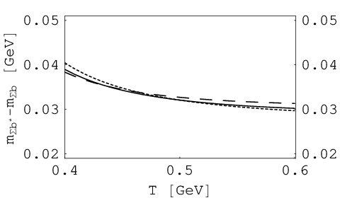
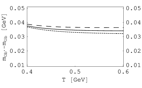
Since the energy gap between the S-wave heavy baryons and their radial/orbital excitations is around 500 MeV, the continuum contribution can be subtracted quite cleanly. We require that the high-order power corrections be less than 30% of the perturbative term to ensure the convergence of the operator product expansion. This condition yields the minimum value for the working region of the Borel parameter. In this work, we choose the working region as $0.4<T<0.6$ GeV.

In Fig. 3-5, we give the dependence of $\bar{\Lambda}$, $\mathcal{K}_{i}$, $\mathcal{S}_{i}$ and mass splitting $m_{B_{b}^{*}}-m_{B_{b}^{\prime}}$ on $T$ and $\omega_{c}$ for $\Sigma_{b}$, $\Xi_{b}^{\prime}$, $\Omega_{b}$. The variation of a sum rule with both $T$ and $\omega_{i}$ contributes to the errors of the extracted value, together with the truncation of the operator product expansion and the uncertainty of vacuum condensate values. We collect the extracted $\bar{\Lambda}$, $\mathcal{K}_{i}$, $\mathcal{S}_{i}$ and mass splitting $m_{B_{c}^{*}}-m_{B_{c}^{\prime}}$ in Table 2.

The masses of bottom baryons from the present work are presented in Table 3. It’s well known that the heavy quark expansion does not work very well for the charmed baryons since the charm quark is not heavy enough to ensure the good convergence of $1/m_{Q}$ expansion. For example, the chromo-magnetic splitting between $\Omega_{c}^{\ast}$ and $\Omega_{c}$ from our work is around 133 MeV, which is much larger than the experimental value 67.4 MeV. However, we still choose to present the masses of S-wave charmed baryons also in Table 3 simply for the sake of comparison with experimental data.

References

• (1) CDF Collaboration, T. Aaltonen, et al., arXiv: 0706.3868 [hep-ex].
• (2) I. V. Gorelov, arXiv:hep-ex/0701056.
• (3) D0 Collaboration, V. Abazov et al., arXiv: 0706.1690 [hep-ex].
• (4) D. Litvintsev, on behalf of the CDF Collaboration, seminar at Fermilab, June 15, 2007, http://theory.fnal.gov/jetp/talks/litvintsev.pdf.
• (5) CDF Collaboration, T. Aaltonen et al., arXiv:0707.0589v1 [hep-ex].
• (6) Babar Collaboration, B. Aubert et al., Phys. Rev. Lett. 97, 232001 (2006); Babar Collaboration, T Schrer, a talk given in Europhysics Conference on High Energy Physics, Manchester, 19-25, July 2007.
• (7) S. Capstick and N. Isgur, Phys. Rev. D 34, 2809 (1986).
• (8) R. Roncaglia, D. B. Lichtenberg and E. Predazzi, Phys. Rev. D 52, 1722 (1995).
• (9) E. E. Jenkins, Phys. Rev. D 54, 4515 (1996).
• (10) N. Mathur, R. Lewis and R. M. Woloshyn, Phys. Rev. D 66, 014502 (2002).
• (11) D. Ebert, R. N. Faustov and V. O. Galkin, Phys. Rev. D 72, 034026 (2005).
• (12) S.M. Gerasyuta and D.V. Ivanov, Nuovo Cim. A 112, 261-276 (1999).
• (13) S. M. Gerasyuta, E. E. Matskevich arXiv:0709.0397.
• (14) E. Bagan, M. Chabab, H. G. Dosch and S. Narison, Phys. Lett. B 278, 367 (1992);i ibid. B 287, 176 (1992).
• (15) M. Karliner and H.J. Lipkin, arXiv: hep-ph/0611306.
• (16) M. Karlinera, B. Keren-Zura, H.J. Lipkina and J.L. Rosner, arXiv: 0706.2163 [hep-ph].
• (17) M. Karliner, B. Keren-Zur, H.J. Lipkin and J.L. Rosner, arXiv:0708.4027 [hep-ph].
• (18) J. L. Rosner, Phys. Rev. D 75, 013009 (2007).
• (19) M. Karlinear and H.J. Lipkin, arXiv: hep-ph/0307243; M. Karlinear and H.J. Lipkin, Phys. Lett. B 575, 249 (2003).
• (20) C. Chen, X.L. Chen, X. Liu, W.Z. Deng and S.L. Zhu, Phys. Rev. D 75, 094017 (2007).
• (21) M.A. Shifman, A.I. Vainshtein and V.I. Zakharov, Nucl. Phys. B 147, 385 (1979); L.J. Reinders, H. Rubinstein and S. Yazaki, Phys. Rep. 127, 1 (1985).
• (22) E. Bagan, M. Chabab, H. G. Dosch and S. Narison, Phys. Lett. B 287, 176 (1992).
• (23) F. S. Navarra and M. Nielsen, Phys. Lett. B 443, 285 (1998).
• (24) E.V. Shuryak, Nucl. Phys. B 198, 83 (1982).
• (25) A.G. Grozin and O.I. Yakovlev, Phys. Lett. B 285, 254 (1992);ibid. B 291, 441 (1992).
• (26) E. Bagan, M. Chabab, H. G. Dosch and S. Narison, Phys. Lett. B 301, 243 (1993).
• (27) Y.B. Dai, C.S. Huang, C. Liu and C.D. Lu, Phys. Lett. B 371, 99 (1996); Y.B. Dai, C.S. Huang, M.Q. Huang and C. Liu, Phys. Lett. B 387, 379 (1996).
• (28) D. W. Wang, M. Q. Huang and C. Z. Li, Phys. Rev. D 65, 094036 (2002).
• (29) S.L. Zhu, Phys. Rev. D 61, 114019 (2000).
• (30) C.S. Huang, A.L. Zhang and S.L. Zhu, Phys. Lett. B 492, 288 (2000).
• (31) D. W. Wang and M. Q. Huang, Phys. Rev. D 68, 034019 (2003).
• (32) Z. G. Wang, arXiv:0704.1106 [hep-ph].
• (33) F.O. Durães and M. Nielsen, arXiv:0708.3030 [hep-ph].
• (34) M. Neubert, Phys. Rept. 245, 259 (1994).
• (35) M. Neubert, Phys. Rev. D 45, 2451 (1992); B. Blok and M. Shifman, Phys. Rev. D 47, 2949 (1993).
• (36) K.C. Yang, W-Y. P. Hwang, E.M. Henley and L.S. Kisslinger, Phys. Rev. D 47, 3001 (1993).
• (37) J. Gasser and H. Leutwyler, Nucl. Phys. B 250, 465 (1985).
• (38) V. Gimenez, V. Lubicz, F. Mescia, V. Porretti and J. Reyes, Eur. Phys. J. C 41, 535 (2005).
• (39) M. Jamin, Phys. Lett. B 538, 71 (2002).
• (40) B.L. Ioffe and K.N. Zyablyuk, Eur. Phys. J. C 27, 229 (2003).
• (41) A.A. Ovchinnikov and A.A. Pivovarov, Sov. J. Nucl. Phys. 48, 721 (1988) [Yad. Fiz. 48, 1135 (1988)].
• (42) W.M. Yao et al., Particle Data Group, J. Phys. G 33, 1 (2006).
• (43) A.H. Hoang, Z. Ligeti and A.V. Manohar, Phys. Rev. Lett. 82, 277 (1999); Phys. Rev. D 59, 074017 (1999).
• (44) W. Lucha, D. Melikhov and S. Simula, Phys. Rev. D 76, 036002 (2007).
• (45) A.A. Ovchinnikov, A.A. Pivovarov and L.R.. Surguladze, Int. J. Mod. Phys. A 6, 2025 (1991).
Refer to caption
Figure 3: The dependences of Λ¯Σb\bar{\Lambda}_{\Sigma_{b}}, 𝒦Σb\mathcal{K}_{\Sigma_{b}}, 𝒮Σb\mathcal{S}_{\Sigma_{b}}, and the mass splitting mΣb∗−mΣbm_{\Sigma_{b}^{*}}-m_{\Sigma_{b}} on TT. Here the dotted, solid and dashed line corresponds to the threshold value ωΣb=1.2,1.3,1.4\omega_{\Sigma_{b}}=1.2,1.3,1.4 GeV respectively.
Figure 4: The dependences of Λ¯Ξb′\bar{\Lambda}_{\Xi_{b}^{\prime}}, 𝒦Ξb′\mathcal{K}_{\Xi_{b}^{\prime}}, 𝒮Ξb′\mathcal{S}_{\Xi_{b}^{\prime}}, and the mass splitting mΞb∗−mΞb′m_{\Xi_{b}^{*}}-m_{\Xi_{b}^{\prime}} on TT. The dotted, solid and dashed line corresponds to ωΞb′=1.3,1.4,1.5\omega_{\Xi_{b}^{\prime}}=1.3,1.4,1.5 GeV respectively.
Figure 5: The dependences of Λ¯Ωb\bar{\Lambda}_{\Omega_{b}}, 𝒦Ωb\mathcal{K}_{\Omega_{b}}, 𝒮Ωb\mathcal{S}_{\Omega_{b}}, and the mass splitting mΩb∗−mΩbm_{\Omega_{b}^{*}}-m_{\Omega_{b}} on TT. The dotted, solid and dashed line corresponds to ωΩb=1.45,1.55,1.65\omega_{\Omega_{b}}=1.45,1.55,1.65 GeV respectively.