跳到论文正文
W Papers独立论文阅读器 arXiv:0709.4506 论文正文 计算阅读时间 · 0%
引用这篇论文根据当前论文元数据生成,正式投稿前建议核对。


License: Assumed arXiv.org perpetual non-exclusive license
arXiv:0709.4506v1 [cs.IT] 27 Sep 2007

Optimum Diversity-Multiplexing Tradeoff in the Multiple Relays Network Financial supports provided by Nortel, and the corresponding matching funds by the Federal government: Natural Sciences and Engineering Research Council of Canada (NSERC) and Province of Ontario: Ontario Centres of Excellence (OCE) are gratefully acknowledged.

Shahab Oveis Gharan    Alireza Bayesteh       Amir K. Khandani Affiliation: Coding & Signal Transmission Laboratory Affiliation: [-5pt] Department of Electrical & Computer Engineering Affiliation: [-5pt] University of Waterloo Affiliation: [-5pt] Waterloo, ON, N2L 3G1 Affiliation: [-5pt] shahab, alireza, khandani@cst.uwaterloo.ca
Abstract

In this paper, a multiple-relay network in considered, in which KK single-antenna relays assist a single-antenna transmitter to communicate with a single-antenna receiver in a half-duplex mode. A new Amplify and Forward (AF) scheme is proposed for this network and is shown to achieve the optimum diversity-multiplexing trade-off curve.

I System Model

The system , as in [1], [2], and [3], consists of KK relays assisting the transmitter and the receiver in the half-duplex mode, i.e. in each time, the relays can either transmit or receive. The channels between each two node is assumed to be quasi-static flat Rayleigh-fading, i.e. the channel gains remain constant during a block of transmission and changes independently from one block to another. However, we assume that there is no direct link between the transmitter and the receiver. This assumption is reasonable when the transmitter and the receiver are far from each other or when the receiver is supposed to have connection with just the relay nodes to avoid the complexity of the network. As in [2] and [4], each node is assumed to know the state of its backward channel and, moreover, the receiver is supposed to know the equivalent channel gain from the transmitter to the receiver. No feedback to the transmitting node is permitted. All nodes have the same power constraint. Also, we assume that a capacity achieving gaussian random codebook can be generated at each node of the network. Hence, the code design problem is not considered in this paper.

II Proposed KK-Slot Switching N-sub-block Markovian Scheme (SM)

In the proposed scheme, the entire block of transmission is divided into NN sub-blocks. Each sub-block consists of KK slots. Each slot has T′T^{\prime} symbols. Hence, the entire block consists of T=N​K​T′T=NKT^{\prime} symbols. In order to transmit a message ww, the transmitter selects the corresponding codeword of a gaussian random codebook consisting of 2N​K​T′​r2^{NKT^{\prime}r} codewords of length N​K−1N​K​T\frac{NK-1}{NK}T and transmits the codeword during the first N​K−1NK-1 slots. In each sub-block, each relay receives the signal in one of the slots and transmits the received signal in the next slot. So, each relay is off in K−22\frac{K-2}{2} of time. More precisely, in the kk’ slot of the nn’the sub-block (1≤n≤N,1≤k≤K,n​k≠N​K1\leq n\leq N,1\leq k\leq K,nk\neq NK), the kk’th relay receives the signals the transmitter is sending, and amplifies and forwards it to the receiver in the next slot. The receiver starts receiving the signal from the second slot. After receiving the last slot (N​KNK’th slot) signal, the receiver decodes the transmitted message by using the signal of N​K−1NK-1 slot received from KK relays. It will be shown in the next section that the equivalent point-to-point channel from the transmitter to the receiver would act as a lower-triangular MIMO channel.

III Diversity-Multiplexing Tradeoff

In this section, we show that the proposed method achieves the optimum achievable diversity-multiplexing curve. First, according to the cut-set bound theorem [5], the point-to-point capacity of the uplink channel (the channel from the transmitter to the relays) is an upper-bound for the capacity of this system. Accordingly, the diversity-multiplexing curve of a 1×K1\times K SIMO system which is a straight line from multiplexing gain 11 to the diversity gain KK is an upper-bound for the diversity-multiplexing curve of our system. In this section, we prove that the tradeoff curve of the proposed method achieves the upper-bound and thus, it is optimum. First, we prove the statement for the case that there is no link between the relays. Next, we prove the statement for the general case.

III-A No Interfering Relays

Assume, the link gain between the kk’th relay and the transmitter and the kk’th relay and the receiver are hkh_{k} and gkg_{k}, respectively. Furthermore, assume that there is no link between the relays. Accordingly, at the kk’th relay we have

𝐫k=hk​𝐱+𝐧k,\mathbf{r}_{k}=h_{k}\mathbf{x}+\mathbf{n}_{k}, (1)

where 𝐫k\mathbf{r}_{k} is the received signal vector of the kk’th relay, 𝐱\mathbf{x} is the transmitter signal vector and 𝐧k∼𝒩⁡(0,𝐈T′)\mathbf{n}_{k}\sim\mathcal{N}(0,\mathbf{I}_{T^{\prime}}) is the noise vector of the channel. At the receiver side, we have

𝐲=∑k=1Kgk​𝐭k+𝐳,\mathbf{y}=\sum_{k=1}^{K}{g_{k}\mathbf{t}_{k}}+\mathbf{z}, (2)

where 𝐭k\mathbf{t}_{k} is the transmitted signal vector of the kk’th relay, 𝐲\mathbf{y} is the received signal vector at the receiver side and 𝐳∼𝒩⁡(0,𝐈T′)\mathbf{z}\sim\mathcal{N}(0,\mathbf{I}_{T^{\prime}}) is the noise vector of the downlink channel. The output power constraint 𝔼⁡{‖𝐱‖2},𝔼⁡{‖𝐭k‖2}≤T′​P\mathbb{E}\left\{\left\|\mathbf{x}\right\|^{2}\right\},\mathbb{E}\left\{\left\|\mathbf{t}_{k}\right\|^{2}\right\}\leq T^{\prime}P holds at the transmitter and relays side. To obtain the DM tradeoff curve of the proposed scheme, we are looking for the end-to-end probability of outage from the rate r​log⁡(P)r\log\left(P\right), as PP goes to infinity.

Refer to caption
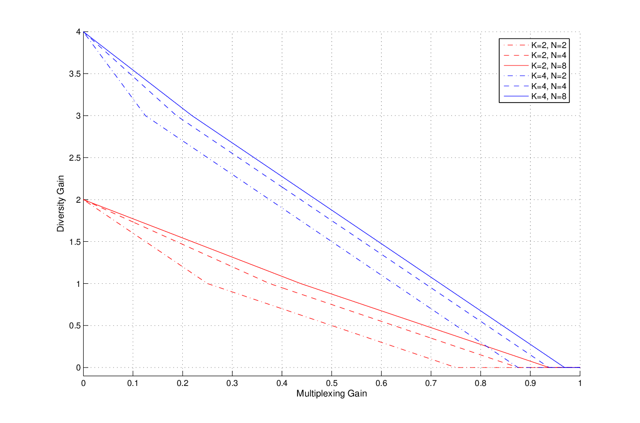
Fig. 1: DM Tradeoff for the proposed Switching Markovian Scheme and various values of (K,N), No interfering relays case
Theorem 1

Assume a half-duplex parallel relay scenario with KK no interfering relays. The proposed SM scheme achieves the diversity gain

dS​M,N​I​(r)=max⁡{0,K⁡(1−r)−1N,K⁡(1−r)−K​rN−1},d_{SM,NI}(r)=\max\left\{0,K\left(1-r\right)-\frac{1}{N},K\left(1-r\right)-\frac{Kr}{N-1}\right\}, (3)

which achieves the optimum achievable DM tradeoff curve do​p​t​(r)=K⁡(1−r)d_{opt}(r)=K(1-r) as N→∞N\to\infty.

Proof.

Let us define 𝐱n,k,𝐧n,k,𝐫n,k,𝐭n,k,𝐳n,k,𝐲n,k\mathbf{x}_{n,k},\mathbf{n}_{n,k},\mathbf{r}_{n,k},\mathbf{t}_{n,k},\mathbf{z}_{n,k},\mathbf{y}_{n,k} as the signal/noise transmitted/received by the transmitter/relay/receiver to the kk’th relay/receiver in the kk’th slot of the nn’th sub-block. Also, let us define (k)≡k−2modK+1(k)\equiv k-2~\mod~K+1 and (n)≡n−⌊(k)K⌋(n)\equiv n-\lfloor{\frac{(k)}{K}}\rfloor. Thus, we have

𝐲n,k\displaystyle\mathbf{y}_{n,k} =\displaystyle= gk​𝐭n,k+𝐳n,k\displaystyle g_{k}\mathbf{t}_{n,k}+\mathbf{z}_{n,k} (4)
=\displaystyle= gk​α(k)​(h(k)​𝐱(n),(k)+𝐧(n),(k))+𝐳n,k,\displaystyle g_{k}{\alpha}_{(k)}\left(h_{(k)}\mathbf{x}_{(n),(k)}+\mathbf{n}_{(n),(k)}\right)+\mathbf{z}_{n,k},

where αk=P|hk|2​P+1{\alpha}_{k}=\frac{P}{|h_{k}|^{2}P+1} is the amplification coefficient performed in the kk’th relay. Defining the event ℰk\mathcal{E}_{k} as the event of outage from the rate r​log⁡(P)r\log(P) in the kk’th sub-channel consisting of the transmitter, the kk’th relay, and the receiver, we have

ℙ​{ℰk}\displaystyle\mathbb{P}\{\mathcal{E}_{k}\} =\displaystyle= ℙ{log[1+P|gk|2|αk|2|hk|2(1+|gk|2|αk|2)−1]≤rlog(P)}\displaystyle\mathbb{P}\left\{\log\left[1+P|g_{k}|^{2}|{\alpha}_{k}|^{2}|h_{k}|^{2}\left(1+|g_{k}|^{2}|{\alpha}_{k}|^{2}\right)^{-1}\right]\leq r\log(P)\right\} (5)
≐\displaystyle\doteq min{sign(r),ℙ{|gk|2|αk|2|hk|2(1+|gk|2|αk|2)−1≤Pr−1}}\displaystyle\min\left\{\mbox{sign}(r),\mathbb{P}\left\{|g_{k}|^{2}|{\alpha}_{k}|^{2}|h_{k}|^{2}\left(1+|g_{k}|^{2}|{\alpha}_{k}|^{2}\right)^{-1}\leq P^{r-1}\right\}\right\}
≐(a)\displaystyle\stackrel{{\scriptstyle(a)}}{{\doteq}} min{sign(r),ℙ{|gk|2|αk|2|hk|2min{12,12​|gk|2​|αk|2}≤Pr−1}}\displaystyle\min\left\{\mbox{sign}(r),\mathbb{P}\left\{|g_{k}|^{2}|{\alpha}_{k}|^{2}|h_{k}|^{2}\min\left\{\frac{1}{2},\frac{1}{2|g_{k}|^{2}|{\alpha}_{k}|^{2}}\right\}\leq P^{r-1}\right\}\right\}
≐(b)\displaystyle\stackrel{{\scriptstyle(b)}}{{\doteq}} min{sign(r),ℙ{|hk|2≤2Pr−1}+ℙ{|gk|2|αk|2|hk|2≤2Pr−1}}\displaystyle\min\left\{\mbox{sign}(r),\mathbb{P}\left\{|h_{k}|^{2}\leq 2P^{r-1}\right\}+\mathbb{P}\left\{|g_{k}|^{2}|{\alpha}_{k}|^{2}|h_{k}|^{2}\leq 2P^{r-1}\right\}\right\}
≐(c)\displaystyle\stackrel{{\scriptstyle(c)}}{{\doteq}} min{sign(r),P−(1−r)+ℙ{|gk|2min{12,|hk|2​P2}≤2Pr−1}}\displaystyle\min\left\{\mbox{sign}(r),P^{-(1-r)}+\mathbb{P}\left\{|g_{k}|^{2}\min\left\{\frac{1}{2},\frac{|h_{k}|^{2}P}{2}\right\}\leq 2P^{r-1}\right\}\right\}
≐(d)\displaystyle\stackrel{{\scriptstyle(d)}}{{\doteq}} min{sign(r),P−(1−r)+ℙ{|gk|2≤4Pr−1}+ℙ{|gk|2|hk|2≤4Pr−2}}\displaystyle\min\left\{\mbox{sign}(r),P^{-(1-r)}+\mathbb{P}\left\{|g_{k}|^{2}\leq 4P^{r-1}\right\}+\mathbb{P}\left\{|g_{k}|^{2}|h_{k}|^{2}\leq 4P^{r-2}\right\}\right\}
≐(e)\displaystyle\stackrel{{\scriptstyle(e)}}{{\doteq}} min⁡{sign​(r),P−(1−r)},\displaystyle\min\left\{\mbox{sign}(r),P^{-(1-r)}\right\},

where sign​(r)\mbox{sign}(r) is the sign function, i.e. sign​(r)=1,r≥0,sign​(r)=0,r<0\mbox{sign}(r)=1,r\geq 0,\mbox{sign}(r)=0,r<0. Here, (a) follows from the fact that 11+|gk|2​|αk|2≐min⁡{12,12​|gk|2​|αk|2}\frac{1}{1+|g_{k}|^{2}|{\alpha}_{k}|^{2}}\doteq\min\left\{\frac{1}{2},\frac{1}{2|g_{k}|^{2}|{\alpha}_{k}|^{2}}\right\}, (b) and (d) follow from the union bound inequality, (c) follows from the fact that |αk|2​|hk|2≐min⁡{12,|hk|2​P2}|{\alpha}_{k}|^{2}|h_{k}|^{2}\doteq\min\left\{\frac{1}{2},\frac{|h_{k}|^{2}P}{2}\right\} and the pdf distribution of the rayleigh-fading parameter near zero, and (e) follows from the fact that the product of two independent rayleigh-fading parameters behave as a rayleigh-fading parameter near zero. (5) shows that each sub-channel’s tradeoff curve performs as a single-antenna point-to-point channel.

Defining Rk​(P)R_{k}(P) as the random variable showing the rate of the kk’th sub-channel consisting of the transmitter, the kk’th relay, and the receiver in terms of PP, the outage event of the entire channel from the r​log⁡(P)r\log(P), the event ℰ\mathcal{E}, is equal to

ℙ{ℰ}=ℙ{N∑k=1K−1Rk(P)+(N−1)RK(P)≤NKrlog(P)}\mathbb{P}\left\{\mathcal{E}\right\}=\mathbb{P}\left\{N\sum_{k=1}^{K-1}{R_{k}(P)}+(N-1)R_{K}(P)\leq NKr\log(P)\right\} (6)

Assuming Rk​(P)=rk​log⁡(P)R_{k}(P)=r_{k}\log(P), we have

ℙ{ℰ}≐ℙ{N∑k=1K−1rk+(N−1)rK≤NKr}\mathbb{P}\left\{\mathcal{E}\right\}\doteq\mathbb{P}\left\{N\sum_{k=1}^{K-1}{r_{k}}+(N-1)r_{K}\leq NKr\right\} (7)

ℙ{Rk(P)≤rklog(P)}\mathbb{P}\left\{R_{k}(P)\leq r_{k}\log(P)\right\} is known by (5). Defining the region ℛ\mathcal{R} as

ℛ={(r1,r2,⋯,rK)|0≤rk≤1,N∑k=1K−1rk+(N−1)rK≤NKr}\mathcal{R}=\left\{\left(r_{1},r_{2},\cdots,r_{K}\right)|0\leq r_{k}\leq 1,N\sum_{k=1}^{K-1}{r_{k}}+(N-1)r_{K}\leq NKr\right\} (8)

it is easy to check that all the vectors (r1,r2,⋯,rK)\left(r_{1},r_{2},\cdots,r_{K}\right) that result in the outage event almost surely lie in ℛ\mathcal{R}. In fact, according to (5), for all kk we know rk≥0r_{k}\geq 0. Also, for rk>1r_{k}>1, ℙ{Rk(P)≥rklog(P)}≤e−Pr−1\mathbb{P}\left\{R_{k}(P)\geq r_{k}\log(P)\right\}\leq e^{-P^{r-1}} which is exponential in terms of PP. Hence, rk>1r_{k}>1 can be disregarded for the outage region. As a result, ℙ{ℰ}≐ℙ{𝐫∈ℛ}\mathbb{P}\left\{\mathcal{E}\right\}\doteq\mathbb{P}\left\{\mathbf{r}\in\mathcal{R}\right\}.

On the other hand, by (5) and the fact that rkr_{k}’s are independent, we have

ℙ⁡{r1≤r10,r2≤r20,⋯,rK≤rK0}≐P−(K−∑k=1Krk0)\mathbb{P}\left\{r_{1}\leq r_{1}^{0},r_{2}\leq r_{2}^{0},\cdots,r_{K}\leq r_{K}^{0}\right\}\doteq P^{-\left(K-\sum_{k=1}^{K}{r_{k}^{0}}\right)} (9)

Now, we show that ℙ​{ℰ}≐P−min𝐫∈ℛ⁡K−𝟏⋅𝐫\mathbb{P}\left\{\mathcal{E}\right\}\doteq P^{-\min_{\mathbf{r}\in\mathcal{R}}{K-\mathbf{1}\cdot\mathbf{r}}}. First of all, by taking derivative of (9) with respect to r1,r2,⋯,rKr_{1},r_{2},\cdots,r_{K}, it is easy to see that the probability density function of 𝐫\mathbf{r} behaves the same as the probability function in (9), i.e. fr​(𝐫)≐P−(K−𝟏⋅𝐫)f_{r}(\mathbf{r})\doteq P^{-\left({K-\mathbf{1}\cdot\mathbf{r}}\right)}. Hence, the outage probability is equal to

ℙ​{ℰ}\displaystyle\mathbb{P}\left\{\mathcal{E}\right\} ≐\displaystyle\doteq ∫𝐫∈ℛfr​(𝐫)​𝑑𝐫\displaystyle\int_{\mathbf{r}\in\mathcal{R}}{f_{r}(\mathbf{\mathbf{r}})d\mathbf{r}} (10)
≤˙\displaystyle\dot{\leq} v​o​l​(ℛ)​P−min𝐫∈ℛ⁡K−𝟏⋅𝐫\displaystyle vol(\mathcal{R})P^{-\min_{\mathbf{r}\in\mathcal{R}}{K-\mathbf{1}\cdot\mathbf{r}}}
≐(a)\displaystyle\stackrel{{\scriptstyle(a)}}{{\doteq}} P−min𝐫∈ℛ⁡K−𝟏⋅𝐫\displaystyle P^{-\min_{\mathbf{r}\in\mathcal{R}}{K-\mathbf{1}\cdot\mathbf{r}}}

Here, (a) follows from the fact that ℛ\mathcal{R} is a fixed bounded region whose volume is independent of PP. On the other hand, by continuity of P−(K−𝟏⋅𝐫)P^{-\left({K-\mathbf{1}\cdot\mathbf{r}}\right)} over 𝐫\mathbf{r}, we have ℙ​{ℰ}​≥˙​P−min𝐫∈ℛ⁡K−𝟏⋅𝐫\mathbb{P}\left\{\mathcal{E}\right\}\dot{\geq}P^{-\min_{\mathbf{r}\in\mathcal{R}}{K-\mathbf{1}\cdot\mathbf{r}}} which combining with (10), results into ℙ​{ℰ}≐P−min𝐫∈ℛ⁡K−𝟏⋅𝐫\mathbb{P}\left\{\mathcal{E}\right\}\doteq P^{-\min_{\mathbf{r}\in\mathcal{R}}{K-\mathbf{1}\cdot\mathbf{r}}}. Defining l⁡(𝐫)=K−𝟏⋅𝐫l(\mathbf{r})=K-\mathbf{1}\cdot\mathbf{r}, we have to solve the following linear programming optimization problem min𝐫∈ℛ⁡l⁡(𝐫)\min_{\mathbf{r}\in\mathcal{R}}{l(\mathbf{r})}. Notice that the region ℛ\mathcal{R} is defined by a set of linear inequality constraints. To solve the problem, we have

l⁡(𝐫)\displaystyle l(\mathbf{r}) ≥(a)\displaystyle\stackrel{{\scriptstyle(a)}}{{\geq}} max⁡{0,K−N​K​r+rKN,K−N​K​r−∑k=1K−1rkN−1}\displaystyle\max\left\{0,K-\frac{NKr+r_{K}}{N},K-\frac{NKr-\sum_{k=1}^{K-1}r_{k}}{N-1}\right\} (11)
≥(b)\displaystyle\stackrel{{\scriptstyle(b)}}{{\geq}} max⁡{0,K⁡(1−r)−1N,K⁡(1−r)−K​rN−1}.\displaystyle\max\left\{0,K(1-r)-\frac{1}{N},K(1-r)-\frac{Kr}{N-1}\right\}.

Here, (a) follows from the inequality constraint in (8) governing ℛ\mathcal{R}, and (b) follows from the fact that rK≤1r_{K}\leq 1 and ∀k<K:rk≥0\forall k<K:r_{k}\geq 0. Now, we partition the range 0≤r≤10\leq r\leq 1 into three intervals. First, in the case that r>1−1N​Kr>1-\frac{1}{NK}, the feasible point 𝐫=𝟏\mathbf{r}=\mathbf{1} achieves the lower bound 00. Second, in the case that r<1K−1N​Kr<\frac{1}{K}-\frac{1}{NK}, the feasible point 𝐫=(0,0,⋯,0,N​K​rN−1)\mathbf{r}=\left(0,0,\cdots,0,\frac{NKr}{N-1}\right), achieves the lower bound K⁡(1−r)−K​rN−1K(1-r)-\frac{Kr}{N-1}. Finally, in the case that 1K−1N​K≤r≤1−1N​K\frac{1}{K}-\frac{1}{NK}\leq r\leq 1-\frac{1}{NK}, The lower bound K⁡(1−r)−1NK(1-r)-\frac{1}{N} is achievable by the feasible point 𝐫,∀k<K:rk=N​K​r−N+1N⁡(K−1),rK=1\mathbf{r},\forall k<K:~r_{k}=\frac{NKr-N+1}{N(K-1)},r_{K}=1. Hence, we have min𝐫∈ℛ⁡l⁡(𝐫)=max⁡{0,K⁡(1−r)−1N,K⁡(1−r)−K​rN−1}\min_{\mathbf{r}\in\mathcal{R}}l(\mathbf{r})=\max\left\{0,K(1-r)-\frac{1}{N},K(1-r)-\frac{Kr}{N-1}\right\}. This completes the proof. ∎

Remark - It is worth noting that as long as the graph G⁡(V,E)G(V,E) whose vertices are the relay nodes and edges are the non interfering relay node pairs includes a hamiltonian cycle 11 1 By hamiltonian cycle, we mean a simple cycle v1v2⋯vKv1v_{1}v_{2}\cdots v_{K}v_{1} that goes exactly one time through each vertex of the graph., the result of this subsection remains valid.

III-B General Case

In the general case, an interference term due to the neighboring relay adds at the receiver antenna of each relay.

𝐫k=hk​𝐱+i(k)​𝐭(k)+𝐧k,\mathbf{r}_{k}=h_{k}\mathbf{x}+i_{(k)}\mathbf{t}_{(k)}+\mathbf{n}_{k}, (12)

where i(k)i_{(k)} is the interference link gain between the kk’th and (k)(k)’th relays. Hence, the amplification coefficient is bounded as αk≤PP⁡(|hk|2+|i(k)|2)+1\alpha_{k}\leq\frac{P}{P\left(\left|h_{k}\right|^{2}+\left|i_{(k)}\right|^{2}\right)+1}. Here, we observe that in the case that αk>1\alpha_{k}>1, the noise nkn_{k} at the receiving side of the kk’th relay can be boosted at the receiving side of the next relay. Hence, we bound the amplification coefficient as αk=min⁡{1,PP⁡(|hk|2+|i(k)|2)+1}\alpha_{k}=\min\left\{1,\frac{P}{P\left(\left|h_{k}\right|^{2}+\left|i_{(k)}\right|^{2}\right)+1}\right\}. In this way, it is guaranteed that the noise of relays are not boosted up through the system. This is at the expense working with the output power less than PP. On the other hand, we know that almost surely 22 2 By almost surely, we mean its probability is greater than 1−P−δ1-P^{-\delta}, for all values of δ\delta. |hk|2,|i(k)|2​≤˙​1\left|h_{k}\right|^{2},\left|i_{(k)}\right|^{2}\dot{\leq}1. Hence, almost surely we have αk≐1\alpha_{k}\doteq 1. Another change we make in this part is that we assume that the entire time of transmission consists of N​K+1NK+1 slots, and the transmitter sends the data during the first N​KNK slots while the relays send in the last N​KNK slots (from the second slot up to the N​K+1NK+1’th slot). Hence, we have T=(N​K+1)​T′T=(NK+1)T^{\prime}. This assumption makes our analysis easier and the lower bound on the diversity curve tighter. Now, we prove the main theorem of this section.

Theorem 2

Consider a half-duplex multiple relays scenario with KK interfering relays whose gains are independent rayleigh fading variables. The proposed SM scheme achieves the diversity gain

dS​M,I​(r)≥max⁡{0,K⁡(1−r)−rN},d_{SM,I}(r)\geq\max\left\{0,K\left(1-r\right)-\frac{r}{N}\right\}, (13)

which achieves the optimum achievable DM tradeoff curve do​p​t​(r)=K⁡(1−r)d_{opt}(r)=K(1-r) as N→∞N\to\infty.

Proof.

First, we show that the entire channel matrix acts as a lower triangular matrix. At the receiver side, we have

𝐲n,k\displaystyle\mathbf{y}_{n,k} =\displaystyle= gk​𝐭n,k+𝐳n,k\displaystyle g_{k}\mathbf{t}_{n,k}+\mathbf{z}_{n,k} (14)
=\displaystyle= gk​α(k)​(∑0<n1,k1,n1​(K+1)+k1<n⁡(K+1)+kpn−n1,k,k1​(hk1​𝐱n1,k1+𝐧n1,k1))+𝐳n,k\displaystyle g_{k}\alpha_{(k)}\left(\sum_{0<n_{1},k_{1},n_{1}(K+1)+k_{1}<n(K+1)+k}{p_{n-n_{1},k,k_{1}}\left(h_{k_{1}}\mathbf{x}_{n_{1},k_{1}}+\mathbf{n}_{n_{1},k_{1}}\right)}\right)+\mathbf{z}_{n,k}

Here, pn,k,k1p_{n,k,k_{1}} has the following recursive formula p0,k,k=1,pn,k,k1=i(k)​α(k)​p(n),(k),k1p_{0,k,k}=1,p_{n,k,k_{1}}=i_{(k)}\alpha_{(k)}p_{(n),(k),k_{1}}. Defining the square N​K×N​KNK\times NK matrices as 𝐆=𝐈N⊗diag​{g1,g2,⋯,gK}\mathbf{G}=\mathbf{I}_{N}\otimes\textit{diag}\left\{g_{1},g_{2},\cdots,g_{K}\right\}, 𝐇=𝐈N⊗diag​{h1,h2,⋯,hK}\mathbf{H}=\mathbf{I}_{N}\otimes\textit{diag}\left\{h_{1},h_{2},\cdots,h_{K}\right\}, 𝛀=𝐈N⊗diag​{α1,α2,⋯,αK}\mathbf{\Omega}=\mathbf{I}_{N}\otimes\textit{diag}\left\{\alpha_{1},\alpha_{2},\cdots,\alpha_{K}\right\}, and

𝐅=(1000…p0,2,1100…p0,3,1p0,3,210…⋮⋮⋮⋮⋱pN−1,K,1pN−1,K,2…p0,K,K−11,)\mathbf{F}=\left(\begin{array}[]{ccccc}1&0&0&0&\ldots\\ p_{0,2,1}&1&0&0&\ldots\\ p_{0,3,1}&p_{0,3,2}&1&0&\ldots\\ \vdots&\vdots&\vdots&\vdots&\ddots\\ p_{N-1,K,1}&p_{N-1,K,2}&\ldots&p_{0,K,K-1}&1\end{array},\right) (15)

where ⊗\otimes is the Kronecker product[6] of matrices and 𝐈N\mathbf{I}_{N} is the N×NN\times N identity matrix, and the N​K×1NK\times 1 vectors 𝐱⁡(s)=[x1,1​(s),x1,2​(s),⋯,xN,K​(s)]T\mathbf{x}\left(s\right)=[x_{1,1}(s),x_{1,2}(s),\cdots,x_{N,K}(s)]^{T}, 𝐧⁡(s)=[n1,1​(s),n1,2​(s),⋯,nN,K​(s)]T\mathbf{n}\left(s\right)=\left[n_{1,1}\left(s\right),n_{1,2}(s),\cdots,n_{N,K}(s)\right]^{T}, 𝐳⁡(s)=[z1,2​(s),z1,3​(s),⋯,zN+1,1​(s)]T\mathbf{z}\left(s\right)=[z_{1,2}(s),z_{1,3}(s),\cdots,z_{N+1,1}(s)]^{T}, and 𝐲⁡(s)=[y1,2​(s),y1,3​(s),⋯,yN+1,1​(s)]T\mathbf{y}\left(s\right)=[y_{1,2}(s),y_{1,3}(s),\cdots,y_{N+1,1}(s)]^{T}, we have

𝐲⁡(s)=𝐆​𝛀​𝐅​(𝐇𝐱⁡(s)+𝐧⁡(s))+𝐳⁡(s).\mathbf{y}\left(s\right)=\mathbf{G}\mathbf{\Omega}\mathbf{F}\left(\mathbf{H}\mathbf{x}\left(s\right)+\mathbf{n}\left(s\right)\right)+\mathbf{z}\left(s\right). (16)

Here, we observe that the matrix of the entire channel acts as a lower triangular matrix of a N​K×N​KNK\times NK MIMO channel whose noise is colored. The probability of outage of such a channel for the multiplexing gain rr is defined as

ℙ{ℰ}=ℙ{log|𝐈K​N+P𝐇T𝐇TH𝐏n−1|≤(NK+1)rlog(P)},\mathbb{P}\left\{\mathcal{E}\right\}=\mathbb{P}\left\{\log\left|\mathbf{I}_{KN}+P\mathbf{H}_{T}\mathbf{H}_{T}^{H}\mathbf{P}_{n}^{-1}\right|\leq(NK+1)r\log\left(P\right)\right\}, (17)

where 𝐏N=𝐈N​K+𝐆​𝛀​𝐅𝐅H​𝛀H​𝐆H\mathbf{P}_{N}=\mathbf{I}_{NK}+\mathbf{G}\mathbf{\Omega}\mathbf{F}\mathbf{F}^{H}\mathbf{\Omega}^{H}\mathbf{G}^{H}, and 𝐇T=𝐆​𝛀​𝐅𝐇\mathbf{H}_{T}=\mathbf{G}\mathbf{\Omega}\mathbf{F}\mathbf{H}. Assume |h⁡(k)|2=P−μ⁡(k)|h(k)|^{2}=P^{-\mu(k)}, |g⁡(k)|2=P−ν⁡(k)|g(k)|^{2}=P^{-\nu(k)}, |i⁡(k)|2=P−ω⁡(k)|i(k)|^{2}=P^{-\omega(k)}, and ℛ\mathcal{R} as the region in ℝ3​K\mathbb{R}^{3K} that defines the outage event ℰ\mathcal{E} in terms of the vector [μ,ν,ω][\mathbf{\mu},\mathbf{\nu},\mathbf{\omega}], where μ=[μ(1)μ(2)⋯μ(K)]T,ν=[ν(1)ν(2)⋯ν(K)]T,ω=[ω(1)ω(2)⋯ω(K)]T\mathbf{\mu}=\left[\mu(1)\mu(2)\cdots\mu(K)\right]^{T},\mathbf{\nu}=\left[\nu(1)\nu(2)\cdots\nu(K)\right]^{T},\mathbf{\omega}=\left[\omega(1)\omega(2)\cdots\omega(K)\right]^{T}. The probability distribution function (and also the inverse of cumulative distribution function) decays exponentially as P−P−δP^{-P^{-\delta}} for positive values of δ\delta. Hence, the outage region ℛ\mathcal{R} is almost surely equal to ℛ+=ℛ​⋂ℝ+3​K\mathcal{R}_{+}=\mathcal{R}\bigcap\mathbb{R}_{+}^{3K}. Now, we have

ℙ​{ℰ}\displaystyle\mathbb{P}\left\{\mathcal{E}\right\} ≤(a)\displaystyle\stackrel{{\scriptstyle(a)}}{{\leq}} ℙ{|𝐇T|2|𝐏n|−1≤P−N​K​(1−r)+r}\displaystyle\mathbb{P}\left\{\left|\mathbf{H}_{T}\right|^{2}\left|\mathbf{P}_{n}\right|^{-1}\leq P^{-NK\left(1-r\right)+r}\right\} (18)
≤(b)\displaystyle\stackrel{{\scriptstyle(b)}}{{\leq}} ℙ{−N∑k=1Kμ(k)+ν(k)−min{0,μ(k),ω((k))}+\displaystyle\mathbb{P}\left\{-N\sum_{k=1}^{K}{\mu(k)+\nu(k)-\min\left\{0,\mu(k),\omega((k))\right\}}+\right.
N​K​log⁡(3)−log⁡|𝐏N|log⁡(P)≤−NK(1−r)+r}\displaystyle\frac{NK\log(3)-\log\left|\mathbf{P}_{N}\right|}{\log\left(P\right)}\leq-NK(1-r)+r\Bigg\}
≤˙(c)\displaystyle\stackrel{{\scriptstyle(c)}}{{\dot{\leq}}} ℙ{NKlog⁡(3)−log⁡(N2​K2+1)log⁡(P)+NK(1−r)−r≤N∑k=1Kμ(k)+ν(k),\displaystyle\mathbb{P}\left\{NK\frac{\log(3)-\log(N^{2}K^{2}+1)}{\log(P)}+NK\left(1-r\right)-r\leq N\sum_{k=1}^{K}{\mu(k)+\nu(k)},\right.
μ(k),ν(k),ω(k)≥0}.\displaystyle\mu(k),\nu(k),\omega(k)\geq 0\Bigg\}.

Here, (a) follows from the fact that for a positive semidefinite matrix 𝐀\mathbf{A} we have |𝐈+𝐀|≥|𝐀|\left|\mathbf{I}+\mathbf{A}\right|\geq\left|\mathbf{A}\right|, (b) follows from the fact that

α⁡(k)=min⁡{1,PP1−μ⁡(k)+P1−ω⁡((k))+1}≥13​min⁡{1,P,Pμ⁡(k),Pω⁡((k))}\alpha(k)=\min\left\{1,\frac{P}{P^{1-\mu(k)}+P^{1-\omega((k))}+1}\right\}\geq\frac{1}{3}\min\left\{1,P,P^{\mu(k)},P^{\omega((k))}\right\}

and assuming PP is large enough such that P≥1P\geq 1, and (c) follows from the fact that α⁡(k)≤1\alpha(k)\leq 1 and accordingly, pn,k,k1≤1p_{n,k,k_{1}}\leq 1, and knowing that the sum of the entries of each row in 𝐅𝐅H\mathbf{F}\mathbf{F}^{H} is less than N2​K2N^{2}K^{2}, we have33 3 This can be verified by the fact that every symmetric real matrix 𝐀\mathbf{A} which has the property that for every ii, ai,i≥∑i≠j|ai,j|a_{i,i}\geq\sum_{i\neq j}|a_{i,j}| is positive semidefinite. 𝐅𝐅H≼N2​K2​𝐈N​K\mathbf{F}\mathbf{F}^{H}\preccurlyeq N^{2}K^{2}\mathbf{I}_{NK}, and ℙ​{ℛ}≐ℙ​{ℛ+}\mathbb{P}\left\{\mathcal{R}\right\}\doteq\mathbb{P}\left\{\mathcal{R}_{+}\right\}, and conditioned on ℛ+\mathcal{R}_{+}, we have min⁡{0,μ⁡(k),ω⁡((k))}=0\min\left\{0,\mu(k),\omega((k))\right\}=0 and ν⁡(k)≥0\nu(k)\geq 0 and consecutively 𝐏N≼(N2​K2+1)​𝐈K​N\mathbf{P}_{N}\preccurlyeq(N^{2}K^{2}+1)\mathbf{I}_{KN}.

On the other hand, we know for vectors μ0,ν0,ω0≥𝟎\mathbf{\mu}^{0},\mathbf{\nu}^{0},\mathbf{\omega}^{0}\geq\mathbf{0}, we have ℙ{μ≥μ0,ν≥ν0,ω≥ω0}≐P−𝟏⋅(μ0+ν0+ω0)\mathbb{P}\left\{\mathbf{\mu}\geq\mathbf{\mu}^{0},\mathbf{\nu}\geq\mathbf{\nu}^{0},\mathbf{\omega}\geq\mathbf{\omega}^{0}\right\}\doteq P^{-\mathbf{1}\cdot\left(\mathbf{\mu}^{0}+\mathbf{\nu}^{0}+\mathbf{\omega}^{0}\right)}. Similarly to the proof of Theorem 1, by taking derivative with respect to μ,ν\mathbf{\mu},\mathbf{\nu} we have fμ,ν(μ,ν)≐P−𝟏⋅(μ+ν)f_{\mathbf{\mu},\mathbf{\nu}}(\mathbf{\mu},\mathbf{\nu})\doteq P^{-\mathbf{1}\cdot\left(\mathbf{\mu}+\mathbf{\nu}\right)} .Defining the lower bound l0l_{0} as l0=log⁡(3)−log⁡(N2​K2+1)log⁡(P)+(1−r)−rN​Kl_{0}=\frac{\log(3)-\log(N^{2}K^{2}+1)}{\log(P)}+\left(1-r\right)-\frac{r}{NK}, the new region ℛ^\hat{\mathcal{R}} as ℛ^={μ,ν≥𝟎,1K𝟏⋅(μ+ν)≥l0}\hat{\mathcal{R}}=\left\{\mathbf{\mu},\mathbf{\nu}\geq\mathbf{0},\frac{1}{K}\mathbf{1}\cdot\left(\mathbf{\mu}+\mathbf{\nu}\right)\geq l_{0}\right\}, the cube ℐ\mathcal{I} as ℐ=[0,K​l0]2​K\mathcal{I}=\left[0,Kl_{0}\right]^{2K}, and for 1≤i≤2​K1\leq i\leq 2K, ℐic=[0,∞)i−1×[Kl0,∞)×[0,∞)2​K−i\mathcal{I}_{i}^{c}=[0,\infty)^{i-1}\times[Kl_{0},\infty)\times[0,\infty)^{2K-i}, we observe

ℙ​{ℰ}\displaystyle\mathbb{P}\left\{\mathcal{E}\right\} ≤˙(a)\displaystyle\stackrel{{\scriptstyle(a)}}{{\dot{\leq}}} ℙ​{ℛ^}\displaystyle\mathbb{P}\{\hat{\mathcal{R}}\} (19)
≤\displaystyle\leq ∫ℛ^​⋂ℐfμ,ν(μ,ν)dμdν+∑i=12​Kℙ{[μ,ν]∈ℛ^∩ℐic}\displaystyle\int_{\mathcal{\hat{R}}\bigcap\mathcal{I}}{f_{\mathbf{\mu},\mathbf{\nu}}\left(\mathbf{\mu},\mathbf{\nu}\right)d\mathbf{\mu}d\mathbf{\nu}}+\sum_{i=1}^{2K}{\mathbb{P}\left\{[\mathbf{\mu},\mathbf{\nu}]\in\mathcal{\hat{R}}\cap\mathcal{I}_{i}^{c}\right\}}
≤˙\displaystyle\dot{\leq} vol(ℛ^∩ℐ)P−min[μ0,ν0]∈ℛ^​⋂ℐ𝟏⋅(μ0+ν0)+2KP−K​l0\displaystyle vol(\mathcal{\hat{R}}\cap\mathcal{I})P^{-\min_{\left[\mathbf{\mu}^{0},\mathbf{\nu}^{0}\right]\in\mathcal{\hat{R}}\bigcap\mathcal{I}}\mathbf{1}\cdot\left(\mathbf{\mu}^{0}+\mathbf{\nu}^{0}\right)}+2KP^{-Kl_{0}}
≐(b)\displaystyle\stackrel{{\scriptstyle(b)}}{{\doteq}} P−K​l0\displaystyle P^{-Kl_{0}}
≐\displaystyle\doteq P−[K⁡(1−r)−rN].\displaystyle P^{-\left[K\left(1-r\right)-\frac{r}{N}\right]}.

Here, (a) follows from (18) and (b) follows from the fact that ℛ^​⋂ℐ\mathcal{\hat{R}}\bigcap\mathcal{I} is a bounded region whose volume is independent of PP. (19) completes the proof. ∎

Refer to caption
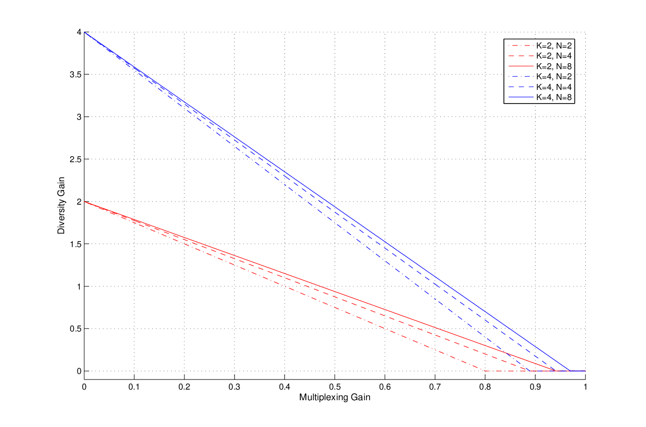
Fig. 2: DM Tradeoff for the proposed Switching Markovian Scheme and various values of (K,N), Interfering relays case

Remark - The statement in the above theorem holds for the general case in which any arbitrary set of relay pairs are non-interfering. Hence, the proposed scheme achieves the upper-bound of the tradeoff curve in the asymptotic case of N→∞N\to\infty for any graph topology on the interfering relay pairs.

Figure (2) shows the D-M tradeoff curve of the scheme for the case of interfering relays and varying number of KK and NN.

References

  • [1] J. N. Laneman, D. N. C. Tse, and G. W. Wornell, “Cooperative diversity in wireless networks: efficient protocols and outage behavior,” IEEE Trans. Inform. Theory, vol. 50, no. 12, pp. 3062–3080, Dec. 2004.
  • [2] K. Azarian, H. El Gamal, and Ph. Schniter, “On the Achievable Diversity-Multiplexing Tradeoff in Half-Duplex Cooperative Channels,” IEEE Trans. Inform. Theory, vol. 51, no. 12, pp. 4152–4172, Dec. 2005.
  • [3] M. Yuksel and E. Erkip, “Cooperative Wireless Systems: A Diversity-Multiplexing Tradeoff Perspective,” IEEE Trans. Inform. Theory, Aug. 2006, under Review.
  • [4] Sh. Yang and J.-C. Belfiore, “A Novel Two-Relay Three-Slot Amplify-and-Forward Cooperative Scheme,” IEEE Trans. Inform. Theory, vol. 51, no. 12, pp. 4152–4172, Dec. 2005.
  • [5] T. M. Cover and J. A. Thomas, Elements of Information Theory. New york: Wiley, 1991.
  • [6] R. A. Horn and C. R. Johnson, Matrix Analysis. Cambridge University Press, 1985.