First, we consider the simplest case where the scalar field $\varphi$ couples only to the real scalar field $\chi$ via the interaction

with $\mu$ being the coupling constant. With this interaction, the decay rate of single particle in the vacuum is given by

In this section, with the interaction given in Eq. (3.1), we discuss how the coherent state decays.

As discussed in the previous section, the decay rate of the coherent state can be related to the imaginary part of the diagonal element of the $T$-matrix $\langle\varphi|\hat{\cal T}|\varphi\rangle$. Importantly, $\langle\varphi|\hat{\cal T}|\varphi\rangle$ is obtained by calculating loop diagrams in the quantum field theory.

At the one-loop level, in other words, neglecting the fluctuation of $\varphi$, $\langle\varphi|\hat{\cal T}|\varphi\rangle$ is expressed as

where the summation over ${\cal F}^{(2p)}$ is for all the possible Feynman diagrams with $2p$ external $\varphi$. With $p$ being fixed, one can find

where $\varphi_{-}$ and $\varphi_{+}$ show up when the field operator $\hat{\varphi}$ is contracted with the creation operator in $|\varphi\rangle$ and the annihilation operator in $\langle\varphi|$, respectively. In order to obtain non-vanishing results, we need to pick up same number of $\varphi_{-}$ and $\varphi_{+}$.

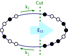
The right-hand side of Eq. (3.4) contains contribution from various Feynman diagrams because $\varphi_{-}$ and $\varphi_{+}$ can be ordered in many ways. In Fig. 1, we show a typical diagram (after imposing the cut). In our notation, we represent the insertion of $\varphi_{-}$ by the white dot $\circ$ while $\varphi_{+}$ by the black dot $\bullet$; non-vanishing diagrams have $p$ black and $p$ white dots. Internal lines are $\chi$-propagator.

Expectation value of $\hat{\cal T}$ for the given diagram ${\cal F}^{(2p)}$ (with $2p$ external $\varphi$ insertion) is given by

where $S_{\cal F}$ is the symmetry factor and

In addition, the momentum flowing on the $I$-th propagator is given by

with

and $\varepsilon_{J}=1$ and $-1$ if the $J$-th $\varphi$ insertion is $\varphi_{-}$ and $\varphi_{+}$, respectively.

The imaginary part of ${\cal T}^{{\cal F}^{(2p)}}$ is obtained by cutting two propagators (see Fig. 1), which corresponds to the replacements of those two propagators by the $\delta$-functions (with a relevant numerical factor):

where

(For details, see Appendix A.) $\Im[{\cal T}^{{\cal F}^{(2p)}}_{i,j}]$ is the contribution from the diagram in which cut is on $i$- and $j$-th propagators. For $\Im[{\cal T}^{{\cal F}^{(2p)}}_{i,j}]$, we define the energy flow from one side of the cut to the other, which we denote $E_{\chi\chi}$; with the following non-negative integer:

the energy flow is given by

Notice that $\Im[{\cal T}^{{\cal F}^{(2p)}}_{i,j}]$ contributes only to the decay rate of the process in which $N_{\varphi}$ of $\varphi$ in the condensation simultaneously annihilate into two $\chi$ because we neglect the fluctuations of the $\varphi$ field. At the perturbative level, such a decay process is kinematically allowed when $E_{\chi\chi}>2m_{\chi}$.

In this and the next subsections, we concentrate on the case where the amplitude of $\varphi$ is small. In this case, the leading-order contribution to the $E_{\varphi}=N_{\varphi}m_{\phi}$ mode is from the diagram with $2N_{\varphi}$ external $\varphi$ with $\varphi_{-}$ and $\varphi_{+}$ being completely separated by the cut. (See Fig. 2.) Concentrating on such a leading-order diagram, the imaginary part of the $T$-matrix element is given by

Constraints from the $\delta$-functions give $\tilde{k}Q_{\varphi}=\frac{1}{2}N_{\varphi}m_{\varphi}^{2}$. Thus,

and hence

where, for $N_{\varphi}m_{\varphi}>2m_{\chi}$, the velocity $\beta_{N_{\varphi}}$ is given by

while $\beta_{N_{\varphi}}=0$ for $N_{\varphi}m_{\varphi}\leq 2m_{\chi}$.

The decay rate of the coherent state $|\varphi\rangle$ per unit volume is evaluated as

and hence is given by

The above expression is consistent with the result given in the study of the parametric resonance [12]. In addition, the decay rate for the $N_{\varphi}=1$ mode is related to the decay rate of single particle, which is given in Eq. (3.2), as

Thus, when the amplitude of $\varphi$ is small, decay of the coherent state can be treated as the decay of individual particles in the condensation, which justifies the conventional treatment of the decay processes of scalar condensations.

We also comment here that the decay rate given in Eq. (3.18) is also derived from the tree-level calculation of the $\chi\chi$ pair creation rate in the external oscillating $\varphi$ field; $\Gamma^{(N_{\varphi})}_{\rm Leading}$ is equal to the production rate of $\chi\chi$ pair per unit volume with total energy of $E_{\chi\chi}=N_{\varphi}m_{\varphi}$. In general, at the leading order of $A_{\varphi}$, the decay rate of the coherent state is also obtained by calculating the tree-level production rate of the final-state particles treating the scalar condensation as an external field. If we consider higher order contributions, however, such a calculation breaks down; treating the scalar condensation as the external field, denominators of some propagators vanish in certain types of diagrams. Notice that, in Eq. (3.9), such a difficulty does not exist. (See also the following discussion.)

In the previous subsection, we have calculated leading-order contributions to the decay rates of each mode in the small amplitude limit. Calculations of the contributions which are higher order in the amplitude are straightforward. In this subsection, we discuss when the small-amplitude expansion breaks down, taking the $N_{\varphi}=1$ mode as an example.

If we calculate $O(|A_{\varphi}|^{2p})$ contributions to the decay rate of such mode, which are from diagrams with $2p$ external $\varphi$ insertions, one finds that the imaginary part of the $T$-matrix element is inversely proportional to the powers of $\beta_{1}$ in the $m_{\varphi}\rightarrow 2m_{\chi}$ limit. First, let us derive such a behavior with explicit calculation.

For the $N_{\varphi}=1$ mode, the most important Feynman diagrams in the $m_{\varphi}\rightarrow 2m_{\chi}$ limit are those in which $\varphi_{+}$ and $\varphi_{-}$ insertions are next to each other. (See Fig. 3.) As we will discuss, other types of diagrams with fixed $p$ have less singular behavior when $\beta_{1}\rightarrow 0$. We also note here that the diagram in Fig. 3 contributes only to the $N_{\varphi}=1$ mode. (The imaginary part of the $T$-matrix vanishes when $N_{\varphi}=0$.)

Taking into account the diagram shown in Fig. 3, the $T$-matrix element becomes

and the imaginary part of ${\cal T}^{(N_{\varphi}=1)}_{\beta_{1}\rightarrow 0}$ is given by

where $(2p-1)!!\equiv\prod_{I=1}^{p}(2I-1)$ for $p\geq 1$, and $(-3)!!\equiv-1$. (For details, see Appendix B.) Hereafter, we neglect $O(\beta_{1}^{7-4p})$ contribution in Eq. (3.21), and the decay rate of the coherent state becomes

As discussed in Appendix B, the inverse powers of $\beta_{1}$ stems from the derivative of the function $B(m_{\phi}^{2};\xi_{i},\xi_{j})$ given in Eq. (A.7) with respect to $\xi_{i}$ or $\xi_{j}$. The order of the derivatives is equal to the number of the propagators whose denominators vanish in the on-shell limit $\xi_{i}\rightarrow m_{\chi}^{2}$ ($i=1-2p$). Number of such propagators is maximized for the diagram given in Fig. 3. Thus, we safely neglect other types of diagrams in studying the case of $\beta_{1}\rightarrow 0$.

As we mentioned, $\Gamma^{(N_{\varphi}=1)}_{\beta_{1}\rightarrow 0}$ becomes singular when $\beta_{1}\rightarrow 0$. In other words, for the $N_{\varphi}=1$ mode, the small-amplitude expansion breaks down when $|A_{\varphi}|$ is comparable to $\mu^{-1}m_{\varphi}^{2}\beta_{1}^{2}$. These behaviors are related to the fact that instability bands appear in the solution to the classical wave equation of the scalar field (i.e., $\chi$ in our argument) which couples to a oscillating scalar field (i.e., $\varphi$). With the interaction given in Eq. (3.1), the wave equation of $\chi$ (with the 3-momentum ${\bf k}$) in the oscillating background is given by the Mathieu equation:

Parametrizing the momentum of $\chi$ as

the lowest instability band in the small-amplitude limit is given by [12]

where

From the study of the parametric resonance, the momentum of $\chi$ produced by the decay of the scalar condensation is in the range given by Eq. (3.25). For the consistency of the calculation, the mass of the initial-state particle $\varphi$ should be large enough so that ${\bf k}^{2}$ is positive even for $\epsilon\sim-\theta$; otherwise, $O(\theta^{2})$ contributions may be also important. This argument gives the limitation of the small-amplitude approximation; $\beta_{1}\gg\theta^{1/2}$ is required, which results in $|A_{\varphi}|\gg\mu^{-1}m_{\varphi}^{2}\beta_{1}^{2}$.

The above argument is supported by the fact that $\Gamma^{(N_{\varphi}=1)}_{\beta_{1}\rightarrow 0}$ given in Eq. (3.22) is equal to the decay rate obtained by the parametric-resonance analysis. Indeed, $\Gamma^{(N_{\varphi}=1)}_{\beta_{1}\rightarrow 0}$ is also expressed as

where, in the first equality, $|{\bf k}|_{\pm}\equiv\frac{1}{2}m_{\varphi}\sqrt{\beta_{1}^{2}\pm\theta}$, and $\lambda^{(N_{\varphi}=1)}=\frac{1}{2}\sqrt{\theta^{2}-\epsilon^{2}}$ is the “growth-rate factor” for the $N_{\varphi}=1$ mode obtained in the study of the Mathieu equation [12]. The equivalence of Eq. (3.22) and Eq. (3.27) can be seen by expanding $\sqrt{\beta_{1}^{2}+\epsilon}$ in the integrand of Eq. (3.27) around $\epsilon=0$ (assuming $\beta_{1}>\theta^{1/2}$). Eq. (3.27) is nothing but the decay rate of the scalar condensation in the small-amplitude limit derived from the parametric-resonance analysis.

Eq. (3.27) (and Eq. (3.18)) also shows the fact that, at least at the small-amplitude limit, the results from the parametric-resonance analysis is obtained in our procedure where the quantum state describing the scalar condensation is postulated to be the coherent state. The equivalence of two approaches is also expected from the fact that the basic equations governing the behavior of the parametric resonance is derived in our framework. In particular, we can calculate the density matrix of the final-state particle $\chi$ in the quantum field theory. We can see that the Mathieu equation shows up in the calculation and that the resultant density matrix is the same as the one obtained in the study of parametric resonance. These subjects will be discussed in the next subsection.

In the classical treatment of the parametric resonant system, it is well known that the Mathieu equation appears as the equation of motion for the $\chi$ field. Thus, the equation is also expected to be obtained in the quantum-field-theory treatment. In this subsection, we show the derivations of the Mathieu equation and the density matrix of $\chi$ explicitly.

Since we are interested in the case where the scalar field $\varphi$ initially forms the scalar condensation oscillating around the minimum of its potential, we describe the initial state (which is taken at $t=0$ in this subsection) as

where the first and second kets represent the states for $\varphi$ and $\chi$, respectively. In addition, $|0\rangle_{\chi}$ is the vacuum of the $\chi$ field. (In the following, we omit the subscript $\chi$.)

For our argument, it is convenient to use the density matrix of the total system in the Schroedinger picture. The density matrix at the time $T$ is simply given by

with $\hat{H}$ being the Hamiltonian of the total system. We consider the properties of $\hat{\rho}_{\rm tot}$ in the coordinate basis:

where $|q\rangle$ and $|X\rangle$ are eigenstates of the field operators $\hat{\varphi}$ and $\hat{\chi}$, respectively:

Then, the density matrix in the coordinate basis, $\rho_{\rm tot}[q,X;q^{\prime},X^{\prime}]\equiv\langle q\otimes X|\hat{\rho}_{\rm tot}(T)|q^{\prime}\otimes X^{\prime}\rangle$, is given by

The kernel is represented in the path integral form as

where $S_{\rm tot}$ is the total action. For the explicit form of the kernel, see [14, 15].

In order to study the behavior of the $\chi$ field, we derive the reduced density matrix of $\chi$ by tracing out $q$ and $q^{\prime}$ variables:

For this purpose, we define

Then, with the use of the properties of the coherent state, we obtain the following relations:

where, in this subsection, we consider the case where $A_{\varphi}$ is real. ($A_{\varphi}$ can be taken to be real with a relevant shift of the time variable.) In addition, $\omega_{\bf k}^{2}={\bf k}^{2}+m^{2}_{\chi}$. In Eqs. (3.37) and (3.38), we omit unimportant numerical constants. Using Eq. (3.37), the reduced density matrix becomes

where

while ${\cal C}$ gives the collision terms:

It can be seen that the periodic perturbation term, $\chi^{2}\cos m_{\varphi}t$, appears in the reduced density matrix. Collision terms, which are proportional to $\chi^{4}$, $\chi^{\prime 4}$, and $\chi^{2}\chi^{\prime 2}$, also appear after the integration. Since no approximation was made to derive the density matrix, the above formula can be used at any amplitude of the $\varphi$ field, $A_{\varphi}$. Furthermore, we can derive the kinetic equation by calculating the correlation function of the $\chi$ field on the reduced density matrix, which allows us to describe the non-linear dynamics of the $\chi$ system, as pointed out in [16].

When the amplitude $A_{\varphi}$ is small enough, we can treat the collision terms as perturbations. Then, the reduced density matrix is, at the leading order calculation, written by using the wave functional of the $\chi$ field:

where

The wave functional is written as a product of an infinite set of wave functions of harmonic oscillators as

where

with the “dot” being the derivative with respect to time. $\Psi[T,X]$ satisfies the boundary condition $\Psi[0,X]=\prod_{\bf k}e^{-\omega_{\bf k}|\tilde{X}_{{\bf k}}|^{2}/2}$ (up to normalization), and its evolution is governed by the wave equation derived from the action given in Eq. (3.45). Thus, $\Psi[T,X]$ is nothing but the wave functional obtained in [12]:

References

- [1] A. H. Guth, Phys. Rev. D 23 (1981) 347.
- [2] K. Sato, Mon. Not. Roy. Astron. Soc. 195 (1981) 467.
- [3] A. D. Linde, Phys. Lett. B 108 (1982) 389.
- [4] A. Albrecht and P. J. Steinhardt, Phys. Rev. Lett. 48 (1982) 1220.
- [5] D. N. Spergel et al. [WMAP Collaboration], Astrophys. J. Suppl. 170 (2007) 377.
- [6] K. Enqvist and M. S. Sloth, Nucl. Phys. B 626 (2002) 395.
- [7] D. H. Lyth and D. Wands, Phys. Lett. B 524 (2002) 5.
- [8] T. Moroi and T. Takahashi, Phys. Lett. B 522 (2001) 215 [Erratum-ibid. B 539 (2002) 303].
- [9] I. Affleck and M. Dine, Nucl. Phys. B 249 (1985) 361.
- [10] L. Kofman, A. D. Linde and A. A. Starobinsky, Phys. Rev. Lett. 73 (1994) 3195.
- [11] Y. Shtanov, J. H. Traschen and R. H. Brandenberger, Phys. Rev. D 51 (1995) 5438.
- [12] M. Yoshimura, Prog. Theor. Phys. 94 (1995) 873.
- [13] L. Kofman, A. D. Linde and A. A. Starobinsky, Phys. Rev. D 56 (1997) 3258.
- [14] R. P. Feynman and F. L. Vernon, Annals Phys. 24 (1963) 118.
- [15] R. P. Feynman and A. R. Hibbs, Quantum Mechanics and Path Integral (McGraw-Hill, New York, 1965).
- [16] S. Matsumoto and M. Yoshimura, Phys. Rev. D 61 (2000) 123509.