Colloids dragged through a polymer solution: experiment, theory and simulation
Abstract
We present micro-rheological measurements of the drag force on colloids pulled through a solution of -DNA (used here as a monodisperse model polymer) with an optical tweezer. The experiments show a violation of the Stokes-Einstein relation based on the independently measured viscosity of the DNA solution: the drag force is larger than expected. We attribute this to the accumulation of DNA infront of the colloid and the reduced DNA density behind the colloid. This hypothesis is corroborated by a simple drift-diffusion model for the DNA molecules, which reproduces the experimental data surprisingly well, as well as by corresponding Brownian dynamics simulations.
Keywords:
DDFT, Brownian particlesI Introduction
Complex fluids in general and colloid-polymer mixtures in particular are an ideal model system for studying of the structure and phase behaviour of multicomponent systems. But they also play a large role in many technological processes such as oil recovery, food science Mezzenga et al. 2005, as well as in most biological systems. For these systems, in addition to the equilibrium properties the dynamics is important. While until recently, research largely focused on bulk rheological properties, it is now understood that interface effects play a significant role. The structure of fluids in general changes in the vicinity of interfaces. In equilibrium situations this is known to lead to fluid structure mediated interactions, i.e., the so-called solvation force or depletion interactions. Theoretically, the concept of depletion interactions in colloid-polymer solutions has been extended to non-equilibrium situations Dzubiella et al. 2003; Krüger and Rauscher 2007. While in equilibrium, these interactions are short ranged (with an interaction range on the order of the particle diameter), they become long ranged in non-equilibrium situations. The reason for this are the long ranged structural changes in the fluid. These structural changes, i.e., an enhanced polymer density infront of the colloid, and a reduced polymer density in its back, also lead to an enhanced friction Squires and Brady 2007; Rauscher et al. 2007. In addition, the structural changes in the vicinity of walls couple back to the rheological properties there, e.g., leading to slip boundary conditions Tuinier and Taniguchi 2005; Tuinier et al. 2006. This, on the other hand, leads to a drag reduction as compared to the expected Stokes drag for the bulk fluid. This work was inspired by dynamic light scattering experiments on colloids in solutions of macro molecules Ullmann et al. 1985; Phillies et al. 1985; Phillies et al. 1987.
In order to elucidate the dynamics of colloids in polymer solutions in more detail, we perform highly controlled experiments on single isolated colloids in -DNA solutions using optical tweezers. This technique allows us to move a colloid through a highly mono-disperse polymer solution at a given velocity and to measure the drag force on the colloid with pN-resolution at the same time. For high DNA concentrations we find a significantly higher drag force than predicted by the Stokes-Einstein theory for the homogeneous solution, however, the force scales approximately linearly with the velocity. We compare the experimental results to a simplified dynamic density functional theory (DDFT) for the non-interacting polymers in a flowing solvent and to Brownian dynamics (BD) simulations.
II Experiment
II.1 Materials and methods
Fig. 1 illustrates the experimental set up, in which one colloid is held by an optical trap surrounded by a polymer solution of -DNA (obtained by New England BioLabs, Germany). An inverted microscope (Axiovert S 100 TV, Carl Zeiss, Jena, Germany) is used and the optical trap is realized with a diode pumped Nd:-YAG laser (1064 nm, 1 Watt, LCS-DTL 322; Laser 2000, Wessling, Germany). Its power is stabilized to achieve long-term stability. Additionally, the profile of the laser-beam was monitored. After passing an optical isolator, a quarter-wave plate is used in order to produce circularly polarized light to exclude effects due to reflection differences of the mirrors between the p- and s-polarisation of the laser light. The beam is expanded and coupled into the back aperture of the microscope objective (Plan-Neofluor 1001.30 Oil, Carl Zeiss, Jena, Germany). Video imaging and the optical position detection are accomplished by a digital camera (KPF 120, Hitachi, Düsseldorf, Germany). The optical stage is positioned in three dimensions with nanometer resolution using piezoactuators (P-5173CD, Physik Instrumente, Karlsruhe, Germany). The sample cell consists of a closed chamber that can be flushed by a syringe pump with varying solutions. The viscosities are measured with an Ostwald viscosimeter at the same temperature (25°C room temperature) and with the same -DNA solutions as used in the experiment.
II.2 Data analysis and calibration
The position of the bead in the optical trap is determined by image analysis (Fig. 2a) Ovryn and Izen 2000; Ovryn 2000. For that a sequence of images is recorded (repetition rate 30 Hz) and analysed based on the Levenberg-Marquardt algorithm (Fig. 2b). As fit function
| (1) | |||||
| (2) |
is used, where is the center position, the optical radius, the amplitude of the profile relative to the background image intensity and a constant to consider the dark diffuse ring around the colloid. A variation of , or in an image sequence indicates the motion in -direction. The calibration of the optical trap is based on Stokes’ law for the pure solvent (here water) as described in detail elsewhere Svoboda and Block 1994. A typical force constant of the trap is 0.085 pN/nm corresponding to forces in the range between 0–50 pN, which can be determined with an accuracy of 0.15 pN.
In the experiments, no sign of irreversible adsorption of -DNA molecules to the colloid was detected. While switching between different flow velocities, the same forces at the same speed were obtained in the range of our uncertainties and after flushing back to pure water the Stokes force of the colloid could be reproduced.

II.3 Experimental results

| 0 | 20 | 30 | |
|---|---|---|---|
| 1.03 mPas | 1.36 mPas | 2.07 mPas | |
| 1.00 mPas | 1.12 mPas | 1.30 mPas | |
| 1.01 mPas | 1.21 mPas | 1.37 mPas | |
| viscosimeter | 1.00 mPas | 1.09 mPas | 1.14 mPas |


| 0 | 20 | 30 | |
|---|---|---|---|


Fig. 3 shows the mesured force on colloids of sizes , , and as a function of the dragging velocity in pure water as well as for DNA concentrations and . Linear fits to the data analyzed in terms of the Stokes drag formula for a colloid of diameter in a DNA solution of viscosity
| (3) |
yield the DNA concentration dependent viscosities in Table 1, shown in Fig. 4. The viscosities obtained in this manner are significantly larger than the viscosities measured in a viscosimeter for the same DNA solution and they increase with the colloid radius . This is a strong indication that on top of the Stokes drag a second mechanism plays a role.
Assuming the viscosities measured in the viscosimeter we can also extract an effective hydrodynamic radius from a fit of Eq. (3) to the data in Fig. 3. The resulting as a function of normalized to the nominal colloid radius is shown in Table 2 and Fig. 5. increases with but it also varies with : the value for m is much larger than the values for the smaller colloids. If the increase of was due to adsorption of DNA molecules to the colloid we would expect the absolute increase of to a first approximation to be independent of .
The molecular weight of a -DNA molecule is and its contour length is about , leading to a radius of gyration of roughly . This corresponds roughly to a hydrodynamic radius of . Based on the hydrodynamic radius and the radius of gyration we get molecular volumes and , respectively. For the highest DNA concentrations used in the experiment, i.e., this corresponds to volume packing fractions of 14% and 50%, respectively. With this, we can extract the intrinsic viscosity of the DNA solution from the viscosimeter data and get . Assuming the intrinsic viscosity for hard sphere suspensions as predicted in Einstein 1911; Ford 1960 we get an effective hydrodynamic radius of .
In Fig. 6 we compare the measured drag forces on the colloids with the predictions given by the Stokes equation (3), assuming the viscosity values measured independently in the viscosimeter. The data is normalized to the measurement in pure water. Apparently, in the DNA solution the drag force is much larger than expected for the increase in viscosity. In addition, the difference of the measured force to the prediction assuming Stokes’ equation (3) with the viscosity values measured in the viscosimeter is larger for larger colloids. This is also apparent in Figs. 4 and 5, where the spurious viscosity and the effective hydrodynamic radius both increase not only with the DNA concentration but also with the colloid radius.
Fig. 7 shows the drag force normalized to the pulling velocity on a colloid of diameter measured as a function of the DNA-density . The data point at is normalized to the Stokes drag force with the viscosity of water . Clearly, the additional drag due to the presence of the DNA in the solution is not linear in and larger as the drag expected from the increased viscosity. The the errorbars for small velocities in Fig. 7 are large due to the error in the velocity.
In Fig. 8 the measured drag force on the colloid is compared to the Stokes drag force in the DNA solution, see Eq. (3). The forces are to a good approximation linear in . The difference between the drag forces for 20 g/ml DNA and for pure water is only significant for velocities larger than 400 m/s. For 40 g/ml DNA we can observe a significant difference already at velocities larger than 100 m/s. The experimental resolution limits the measurment of the DNA induced drag force to relatively large velocities and to large DNA concentrations. However, Fig. 8(b) clearly shows that the measured drag forces cannot be explained simply by an increased viscosity of the solution.


III Drift-diffusion model
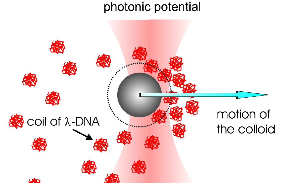
That the drag force on the colloid cannot be explained simply by the increased viscosity of the DNA solution and the dynamics of the DNA in the vicinity of the moving colloid has to be taken into account, which is gouverned by the interplay of direct intermolecular interactions, hydrodynamics, and the internal degrees of freedom of a polymer chain. It has been shown, that an additional drag force due to the rearrangement of solute particles in the vicinity of a dragged colloid can be already obtained in a simple drift diffusion (DD) model Rauscher et al. 2007. Here we employ the same model to calculate this additional drag force and compare it to the experimental values. Within this model, the DNA molecules are idealized as mutually non-interacting particles with a finite hard core interaction radius with the colloid. The origin of this additional force is illustrated in Fig. 9. Due to the repulsion of the DNA coils and the colloid, the center of mass of the DNA coils can approach the colloids surface only up to a distance of roughly , i.e., the radius of gyration, which creates a forbidden zone for the DNA. The solvent molecules, however, are much smaller and enter this zone, such that the solvent flow field has a component normal to the surface of the forbidden zone pointing inwards infront of the colloid and outwards behind the colloid. DNA coils advected with the solvent will therefore accumulate infront of the colloid and their density will be reduced in its back. This inhomogeneous DNA distribution will lead to an inhomogeneous osmotic pressure and therefore to a force on the colloid.

We will quantify the rearrangement of DNA molecules by calculating the average concentration (in units of molecules per volume) near the colloid, which, in the simple drift-diffusion (DD) model described in Squires and Brady 2007; Rauscher et al. 2007, is given by the stationary solution of the Smoluchowski equation
| (4) |
in a frame of reference comoving with the colloid, with the solvent velocity field and the DNA (zero concentration) diffusion constant . In contrast to Ref. Squires and Brady 2007, is not uniform but it is the solution of Stokes’ equation for a sphere of radius translating with velocity through a resting solvent ( for ) (see, e.g., Ref. Landau and Lifshitz 2005 for details),
| (5) |
with the unit vector . As we model the interaction potential between the colloid and the polymers as a hard-sphere potential, the centers of the polymers are excluded from a sphere of radius around the center of the colloid, see Fig. 9. Therefore, the boundary condition for Eq. (4) on this sphere is
| (6) |
i.e., the DNA current normal to the sphere’s surface has to vanish. Far from the colloid, the DNA density should be constant, i.e., for . As the mutual interaction between the DNA molecules is neglected, the local pressure on the colloid surface can be calculated from the ideal gas law . Integrating the local pressure over the surface yields the force on the colloid.
The solution of Eq. (4) depends only on the dimensionless velocity (the Peclet number) of the colloid and the size ratio of the involved particles . For , i.e., for , the surface of the forbidden zone coincides with the colloid surface and the DNA behaves like a solvent molecule. In this limit the solution of Eq. (4) is , the DNA molecules do not accumulate infront of the colloid and therefore the additional drag force vanishes.
With a hydrodynamic radius of m the Stokes-Einstein relation leads to a diffusion constant . Therefore, the smallest velocities in the experiments () correspond to Peclet numbers larger than 100 (depending on the colloid radius). While for small Eq. (4) can be solved analytically in linear order in the Peclet number, we have to use numerical methods for the experimental velocities. To this end, we expand the density field in spherical harmonics up to order and obtain a system of ordinary differential equations for the -dependent expansion coefficients which we solved numerically with AUTO 2000 11 1 http://sourceforge.net/projects/auto2000/ (for details, see Ref. Rauscher et al. 2007). For large a fine numerical discretization (large ) is needed since the thickness of the region in front of the colloid in which the DNA density is enhanced decreases with while the density in this region increases with . We therefore use , which allows us to calculate reliable solutions up to . For such high velocities the drag force is well approximated by an affine function (see Fig. 10 and also Ref. Squires and Brady 2007)
| (7) |
which we use to extrapolate to velocities larger than , see Fig. 10. The coefficients for fits to the numerical data in the range for the experimentally relevant values m and m are given in Table 3. In order to calculate also for other values of and to test the sensitivity of our result to variation of we use the linear interpolation of the coefficients and
| (8a) | |||||
| (8b) | |||||

| [m] | |||
|---|---|---|---|
| 0.66 | 0.57 | 3.31 | 0.126 |
| 1.12 | 0.69 | 2.43 | 0.063 |
| 1.50 | 0.75 | 1.76 | 0.036 |
For the ideal gas law which we use to calculate the local osmotic pressure on the colloid surface we need the number density rather than the mass density as used in the experiments. With the molecular weight g we get .
Fig. 8 compares the forces on a colloid of size m predicted by the DD model to the experimental data. Although the difference of the force at a concentration of in pure water (i.e., only the Stokes force) is hardly significant and within the experimental error explained by the enhanced viscosity of the DNA solution (Fig. 8(a)), theory and experiment are in better correspondence (in particular for larger velocities) if one takes into account the force for a DNA radius of m. For higher DNA concentrations (e.g., in Fig. 8(b)), where the measured forces cannot be explained by the increased viscosity, calculated from the DD model for m is too small. A reasonable fit to the data can be obtained for m, however, for this large value the forces predicted for the lower DNA concentrations (see, e.g., Fig. 8(a)) are too large.
The experimentally measured drag force as a function of the DNA concentration as shown in Fig. 7 clearly shows a nonlinearity indicating that interactions among the DNA molecules are relevant for concentrations larger than . The DD model presented in this section does not take these into account. Therefore, Brownian dynamics simulations are performed as presented in the following section.
IV Brownian Dynamics Simulations

We simulate the experiments with colloids of radius m using a Brownian Dynamics (BD) method – also called Langevin Dynamics van Gunsteren et al. 1981. The polymers and the colloid are modeled as hard spheres with their respective radii. For the polymers we use the radius of gyration m. As the polymers drag along most of the water contained in their volume, the polymers are assigned the mass of water contained in a sphere with radius . The number of polymers in the system is chosen such that the number density (rather than the mass density) of the experiments is reproduced. We use a rectangular simulation volume of with periodic boundary conditions in all three directions. For a polymer concentration of 40 g/ml this corresponds to 30592 polymers.
The colloid is trapped in a moving parabolic potential , mimicking the optical tweezer. The potential has a spring constant of pN/nm, which gives a better signal to noise ratio than the experimental value of pN/nm. Figure 11 shows a snapshot of our simulation setup.
In BD, two most important aspects of hydrodynamics felt by the suspended particles are taken into account, namely the Stokes friction and the Brownian motion. Correspondingly, this is done by adding to a molecular dynamics simulation two additional forces. The Langevin equation describes the motion a Brownian particle with radius at position as
| (9) |
where the first term models the Stokes friction in a solvent of viscosity , is the sum of all external forces like gravity, forces excerted by other suspended particles, and, for the colloid, the optical trap. describes the thermal noise which gives rise to the Brownian motion. The random force on different particles is assumed to be uncorrelated, as well as the force on the same particle at different times. It is further assumed to be Gaussian with zero mean. The mean square deviation of the Gaussian (i.e., the amplitude of the correlator) is given by the fluctuation-dissipation theorem as
| (10) |
In order to reduce computation time, physical quantities are rescaled: the simulation is carried out at a lower temperature. To compensate for this, the viscosity of the fluid as well as all energies are scaled by the same factor. In the present simulations, temperature is scaled down by a factor of 37500. This scaling leaves the diffusion constant as well as the relative importance of diffusion and motion caused by external forces unchanged. However, it allows for a much larger time step (in this case 60s) Hecht et al. 2005.
From the simulation data, it is possible to measure the effective polymer concentration around the dragged colloid. To accomplish this, about 600 snapshots of the simulation are taken: Each snapshot is moved, so that the position of the colloid coincides, and the probability for a certain space to be occupied by a polymer is calculated by averaging over all snapshots (200 x 100 bins are used). The picture in Fig. 12a depicts a typical example of a density map for a concentration of 20 g/ml and m/s. It can be observed that there is a region of high polymer concentration infront and at the sides of the colloid whereas the region behind the colloid is not yet completely refilled by the polymers. Figure 12b shows the normalized average density of polymers in the direction of motion for concentrations of 5g/ml and 20 g/ml and =50m/s. Infront of the colloid, a sharp peak can be observed. In addition, on observes density oscillations which are typical for hard sphere suspensions. For high polymer concentrations, the probability is close to 1 to find a polymer infront of the colloid. The region behind the colloid is almost clear of polymers, because polymers did not yet have enough time to relax into this region again.


BD is widely used to simulate suspensions (e.g. Reichhardt and Olson Reichhardt 2006; Reichhardt and Olson Reichhardt 2004a; Reichhardt and Olson Reichhardt 2004b) because it is well understood, not difficult to implement, and needs much less computational resources than a full simulation of the fluid. However, this simulation method does not resolve more complicated hydrodynamic phenomena, in particular long-ranged hydrodynamic interactions among the polymer particles and in particular between the polymers and the colloid. As a result both, the friction and the thermal force excerted on a particle are independent of the position and velocity of the other particles. In the case of a polymer trapped infront of the moving colloid (i.e., if it is dragged along by the colloid), this leads to a considerable overestimation of the friction felt by the colloid: in a BD simulation it feels the friction on itself and the dragged polymer, whereas in reality the friction on the colloid would be significantly reduced because it is in the polymer’s slipstream. In addition, as argued in Ref. Rauscher et al. 2007, the hydrodynamic interaction of the colloid with the polymers is of importance. The solvent molecules flow around the colloid and the resulting flow field advects the polymers around the colloid (see Eq. (5)), therefore significantly reducing the polymer jam infront of the colloid. To compensate for both of these effects we reduced the friction felt by the polymers, i.e., increase their diffusion constant. This does not significantly influence the density distribution outside the interaction region where the polymers are homogeneously distributed.

Our model reproduces very well the linear relation between drag force and the drag velocity for different polymer concentrations. As higher drag velocities require a larger system (even with periodic boundary conditions) and short numerical timesteps, we are limited to about fifty micrometers per second by the available computational resources and time. However, this is not a problem because of the linearity of the drag force with respect to velocity for higher velocities as observed in the experiments. Fig. 8 includes a linear fit to the simulation data for velocities between m/s and m/s, which agrees well with the experimental data.
As in the experiments, with Eq. (3) the measured drag force can be interpreted in terms of an effective viscosity. Fig. 13 shows the dependency of this viscosity on the velocity for pure water and for polymer concentrations of 20g/ml and 40g/ml. Even for a polymer concentration of 40g/ml the viscosity stays constant for drag velocities greater than 30m/s, but for very low velocities, in all three cases we find that the drag force decreases less then linearly. For such low drag velocities the colloid is very near the trap center and thermal fluctuations about the average position are large. An energy of corresponds to a displacement of m, whereas the displacement calculated from the drag force in water at m/s corresponds to a displacement of m. However, these fluctuations should be roughly symmetric with respect to the average colloid position within the trap. However, the force calculated numerically within the framework of the DD model shown in Fig. 10 analyzed in terms of an effective viscosity would also give an increased viscosity for smaller velocities: the slope is larger for smaller values of . Therefore we conclude, that the apparent increase in viscosity as shown in Fig. 13 is at least partially related to the formation of the polymer jam infront of the colloid. However, the dataset for pure water (i.e., without polymers) indicates, that at very low velocities, fluctuations do play a role.
For a fixed drag velocity and varying polymer concentrations, the linear relation between force and concentrations for low polymer concentrations and the stronger nonlinear increase for higher concentrations can also be observed as shown in Fig. 7. The increase in drag force is overestimated as expected if the mobility of the polymers is not increased (as described above). When the mobility of the polymers is increased by a factor of 14.3, however, quantitative agreement is achieved for concentrations up to 40 g/ml. For even higher concentrations, the drag force increases stronger than in the experiments. This is because at high concentrations, a hard sphere suspension has a stronger tendency to jam than a real polymer suspension: polymers are deformable such that, in contrast to hard spheres, they can squeeze past each other. The simulation results for increased polymer mobility indicate that the friction felt by a pair of a colloid and a dragged polymer in the experiment is far less than the sum of the friction forces on a single polymer and colloid, respectively.
V Discussion
The experiments clearly show that the drag force on colloids pulled through a solution of -DNA with an optical tweezer cannot be explained by the Stokes force for the viscosity of the solution. It is much higher and increases non-linearly with the DNA-concentration but approximately linearly with the drag velocity. The resolution of the force measurment is pN and therefore the difference between the forces on the colloid in the solution and in pure water can be measured only for large concentrations or, in the case of smaller concentrations only for large velocities. This limits the overlap between the DD theory and the experiments to the lowest concentration of used in the experiment.
At this concentration, the volume fraction of the solution taken by the DNA coils (based on m) is 0.1 and DNA-DNA interactions can be neglected. The agreement between theory and experiment is very good. For the highest concentration used in the experiments the volume fraction is 0.5 and DNA-DNA interactions have to be taken into account.
In the BD simulations DNA-DNA interactions have been taken into account. As in the experiments and in the DD theory, the drag force increases linearly with the velocity, at least for large velocities. The nonlinear increase of the drag force with the DNA concentration is also observed in the BD simulations. However, since the BD simulations could not take into account hydrodynamic interactions between the colloid and the DNA molecules, the drag force is significantly overestimated. The hydrodynamic flow field around the colloid as shown in Fig. 9 has a component normal to the direction of motion of the colloid which efficiently reduces the number of DNA molecules accumulated infront of the colloid, while it fills the depletion zone at its back. As demonstrated by the excellent agreement with the experimental data, this hydrodynamic interaction between the colloid and the DNA has the same effect as increasing the DNA mobility, here by a factor of 14.3. This is consistent with results of BD simulations of soft particles in a background flow, where the drag force was reduced by a factor of 10 by this hydrodynamic effect Rauscher et al. 2007.
The agreement between theory and experiment for low concentrations but high velocities is particularly remarkable considering the simplicity of the models which neglect many aspects of hydrodynamic interactions or include them in a rather simplistic way (e.g., in terms of an increased viscosity in the DD model). The internal structure of the DNA molecules is neglected in both, the DD model as well as the BD simulations. Apparently, the deformation of the DNA coils in the accumulation region infront of the colloid is not significant. This can be only explained by the proximity of the stagnation point for the solvent flow which limits the normal component of the the solvent velocity field. At this point the shear rate is also smaller than at the colloid’s side, where it goes up to over 700 1/s for . With a relaxation time on the order of 0.1 s Fang et al. 2005 this amount to a Weissenberg number Wi on the order of 70, i.e., much larger than one. Therefore the polymercoils should be significantly distorted and viscoelastic effects are to be expected.
In summary, we present a first direct experimental observation of jamming-induced drag-enhancement on colloids in polymer solutions. First theoretical approaches to this problem as well as the Brownian dynamics simulations presented in this paper contain many simplifications which need to be addressed in the future.
Acknowledgements.
F.K. J.H., and M.R. acknowledge support by the Deutsche Forschungsgemeinschaft within the priority program SPP 1164 “Micro- and Nanofluidics”. J.H. and R.W. also acknowledge fruitful discussions with M. Hecht. The computations were performed at Forschungszentrum Jülich and at the Scientific Supercomputing Center in Karlsruhe.References
- Mezzenga et al. (2005) R. Mezzenga, P. Schurtenberger, A. Burbidge, and M. Michel, Nature Materials 4, 729 (2005).
- Dzubiella et al. (2003) J. Dzubiella, H. Löwen, and C. N. Likos, Phys. Rev. Lett. 91, 248301 (2003).
- Krüger and Rauscher (2007) M. Krüger and M. Rauscher, J. Chem. Phys. 127, 034905 (2007).
- Squires and Brady (2007) T. M. Squires and J. F. Brady, Phys. Fluids 17, 073101 (2007).
- Rauscher et al. (2007) M. Rauscher, M. Krüger, A. Dominguez, and F. Penna (2007).
- Tuinier and Taniguchi (2005) R. Tuinier and T. Taniguchi, J. Phys.: Condens. Matter 17, L9 (2005).
- Tuinier et al. (2006) R. Tuinier, J. K. G. Dhont, and T.-H. Fan, Europhys. Lett. 75, 929 (2006).
- Ullmann et al. (1985) G. S. Ullmann, K. Ullmann, R. M. Lindner, and G. D. J. Phillies, J. Phys. Chem. 89, 692 (1985).
- Phillies et al. (1985) G. D. J. Phillies, G. S. Ullmann, K. Ullmann, and T.-H. Lin, J. Chem. Phys. 82, 5242 (1985).
- Phillies et al. (1987) G. D. J. Phillies, C. Malone, K. Ullmann, G. S. Ullmann, J. Rollings, and L.-P. Yu, Macromolecules 20, 2280 (1987).
- Ovryn and Izen (2000) B. Ovryn and S. H. Izen, J. Opt. Soc. Am. A 17, 1202 (2000).
- Ovryn (2000) B. Ovryn, Experiments in Fluids 29, S175 (2000).
- Svoboda and Block (1994) K. Svoboda and S. M. Block, Ann. Rev. Biophys. Biomol. Structure 23, 247 (1994).
- Einstein (1911) A. Einstein, Annalen der Physik 34, 591 (1911).
- Ford (1960) T. F. Ford, J. Phys. Chem. 64, 1168 (1960).
- Landau and Lifshitz (2005) L. D. Landau and E. M. Lifshitz, Fluid mechanics, vol. 6 of Course of theoretical physics (Elsevier Butterworth-Heinemann, 2005), 2nd ed.
- van Gunsteren et al. (1981) W. F. van Gunsteren, H. J. C. Berendsen, and J. A. C. Rullman, Mol. Phys. 44, 69 (1981).
- Hecht et al. (2005) M. Hecht, J. Harting, T. Ihle, and H. J. Herrmann, Phys. Rev. E 72, 011408 (2005).
- Reichhardt and Olson Reichhardt (2006) C. Reichhardt and C. J. Olson Reichhardt, Phys. Rev. Lett. 96, 028301 (2006).
- Reichhardt and Olson Reichhardt (2004a) C. Reichhardt and C. J. Olson Reichhardt, Phys. Rev. E 69, 041405 (2004a).
- Reichhardt and Olson Reichhardt (2004b) C. Reichhardt and C. J. Olson Reichhardt, Phys. Rev. Lett. 92, 108301 (2004b).
- Fang et al. (2005) L. Fang, H. Hu, and R. G. Larson, J. Rheology 49, 127 (2005).