Microscopic non-equilibrium theory of quantum well solar cells
Abstract
We present a microscopic theory of bipolar quantum well structures in the photovoltaic regime, based on the non-equilibrium Green’s function formalism for a multi band tight binding Hamiltonian. The quantum kinetic equations for the single particle Green’s functions of electrons and holes are self-consistently coupled to Poisson’s equation, including inter-carrier scattering on the Hartree level. Relaxation and broadening mechanisms are considered by the inclusion of acoustic and optical electron-phonon interaction in a self consistent Born approximation of the scattering self energies. Photogeneration of carriers is described on the same level in terms of a self energy derived from the standard dipole approximation of the electron-photon interaction. Results from a simple two band model are shown for the local density of states, spectral response, current spectrum, and current-voltage characteristics for generic single quantum well systems.
pacs
72.30.+w, 73.21.Fg, 73.23.-b, 78.67.DeI Introduction
Since the pioneering work of Barnham and co-workers barnham:90 in the early nineties, the potential efficiency enhancement by the introduction of quantum wells in the intrinsic region of a pin-diode solar cell (Fig. 1) has attracted considerable interest both from the photovoltaic community and within a broad spectrum of fundamental research barnham:02. A consistent and quantitative description of the carrier generation, recombination, relaxation and transport processes in quantum well solar cells (QWSC) requires the combination of a microscopic model for the electronic structure with a formalism for quantum transport in interacting systems. The non-equilibrium Green’s function formalism (NEGF), first introduced by Kadanoff and Baym kadanoff:62 and by Keldysh keldysh:65, together with a tight-binding or Wannier basis meets these requirements and has been sucessfully applied to similar systems such as quantum cascade laserswacker_sl:02; lee_prb:02, infrared photodetectors henrickson:02, carbon nanotube photodiodesstewart:04; guo:06 or resonant tunneling diodes lake:97.

Generation and recombination
1. Photogeneration of electron-hole pairs
5. Radiative recombination
6. Nonradiative recombination (Auger, trap)
Transport
2. Resonant and nonresonant tunneling
3. Thermal escape and sweep-out by built in field
4. Relaxation by inelastic scattering (optical phonons)
The paper is organized as follows: In section II, we introduce the model Hamiltonian in a planar orbital basis and the procedure based on the NEGF formalism to use it in the derivation of physical quantities. Section III presents and discusses typical results of the theory for a generic bipolar quantum well structure. Section V summarizes the paper and provides an outlook to future work.
II Microscopic model for QWSC
II.1 Hamiltonian and basis
The QWSC system is described in terms of the model Hamiltonian
| (1) |
provides ballistic transport: it contains the kinetic energy, the (bulk) band structure and band offsets, and also includes the electrostatic potential from the solution of Poisson’s equation, which corresponds to the consideration of single species carrier-carrier scattering on the Hartree level. The interaction part consists of the terms and for electron-phonon and electron-photon scattering, respectively. Any other kind of interaction, like scattering by ionized impurities, alloy composition inhomogeneities or interface roughness, inter-carrier-scattering beyond the Hartree level, and all non-radiative recombination processes like Auger or trap recombination are contained in additional terms that will not be discussed in this paper, which is focused on the radiative limit.
In layered semiconductors, carrier Bloch states can be represented in terms of linear combinations of planar orbitals chang:81
| (2) | ||||
| (3) |
where is the band index, denotes a set of orthogonal localized orbitals (e.g. in a 10 band model for zinc-blende materialsvogl:83), indicates the layer, which can consist of several different atomic layers, and the (transverse) location within the layer. is a normalization factor and , the transverse and longitudinal wave vectors, respectively. The corresponding field operators are
| (4) | ||||
| (5) |
where () is the annihilation (creation) operator for a fermion in state .
In a planar orbital basis (POB), the Hamiltonian for ballistic transport is expressed as
| (6) |
where contains the on-site energy, the intra-layer couplings (overlap integrals) and the Hartree potential, while denotes the inter-layer coupling.
The operator for carrier-photon interaction reads
| (7) |
with the quantized photon field given by
| (8) |
where is the polarization of the photon in mode and with momentum created by the boson creation and annihilation operators , and is the absorbing volume.
In a first approach, we restrict the discussion to single-mode monochromatic photons of energy and use the standard dipole approximation, which yieldshenrickson:02
| (9) | ||||
| (10) |
where is the polarization and represents the incoming photon flux, which depends on the intensity and the photon energy, and provides photons per absorbing volume and for given optical properties (: dielectric constant, : magnetic permeability). In the POB for a layered system, the Hamiltonian for electron-photon interaction takes the form
| (11) | ||||
| (12) |
In the dipole approximation, has no spatial dependence and thus
| (13) |
where , is the electron charge and its bare mass. The band structure model dependent dipole-matrix elements for the (direct) interband transitions can be written in terms of the tight-binding Hamiltonian as voon:93; graf:95; boykin:01
| (14) | ||||
| (15) |
where . In the case of light incidence normal to the layer, the polarization is purely transverse, and becomes a scalar function of the transverse momentum.
For the interaction of carriers with phonons, which is on the level of a coupling to an equilibrium heat bath, the harmonic approximation provides the interaction term
| (16) |
where characterizes the coupling matrix elements. In the case of a diatomic basis, as in zinc-blende compounds, the corresponding POB interaction Hamiltonian is given by
| (17) | ||||
| (18) |
where the exact form of the coupling element depends again on the band structure model.
II.2 Green’s functions and self-energies
Within the planar orbital basis, the real time non-equilibrium Green’s functions are defined as the non-equilibrium ensemble averages
| (19) | ||||
| (20) | ||||
| (21) | ||||
| (22) |
In steady state, the above Green’s functions depend only on the time difference , and it is thus possible to work with the Fourier transform
| (23) |
The effects of carrier injection and absorption by extended, highly doped contacts acting as reservoirs are absorbed into respective boundary self energies , reflecting the openness of the system and leading to an effective Hamiltonian of the truncated system caroli:71; datta:95; sanvito:99. Since the contacts form equilibrated flat band regions, their propagating and evanescent bulk Bloch states can be determined exactly. The boundary self energy then represents the matching of the planar orbital states in the device to the extended lead modes at the interface of the contacts, corresponding to a quantum transmitting boundary methodlent:90. For instance at the left boundary (), the retarded boundary self energy is given by (see appendix for a detailed derivation)
| (24) |
where specifies the transformation from localized basis to left-travelling Bloch states and is the interlayer propagator for the corresponding bulk modesando:91; bouwen:95; ogawa:99. The lesser and greater self energies are then obtained from the broadening function and the Fermi distribution of the contact characterized by the chemical potential ,
| (25) | ||||
| (26) | ||||
| (27) |
Analogous expressions are found for the right contact.
While the boundary self energies result from an exact treatment, interactions such as carrier-phonon and carrier-photon scattering are included perturbatively in terms of interaction self energies on the level of a self-consistent Born approximation (SCBA). The self energies for both carrier-photon and carrier-phonon are obtained from the Fock term in second order perturbation theory for general carrier-boson interaction. The corresponding Hartree term is neglected at the present stage (see e.g. hyldgaard:94 for an extensive discussion). In the case of the light-matter interaction the Bose-Einstein distribution in the equilibrium bosonic propagator is replaced by the number of photons present in a layer. The lesser and greater self energies read (in full matrix notation)
| (28) |
and the retarded self energy is given by
| (29) |
The principal value in the expression for the retarded self energy is often neglected, since it will only contribute an energy renormalization, but not to relaxation or phase breaking. We will adopt this approximation in the present work.
For the interactions with polar optical phonons, the self energies are then given by (again neglecting the principal value integration in the retarded case)
| (30) | ||||
| (31) |
where is the Bose-Einstein distribution for equilibrium bosons with energy and at lattice temperature . is a basis dependent function of the coupling parameters, spatial structure and momentum transfer.
For low energy (elastic) scattering with acoustic phonons and high lattice temperature, the expression for the equilibrium phonon propagator can be simplified to provide the (block-)diagonal, momentum independent self energies
| (32) |
A detailed derivation of the electron-phonon self energies for zinc-blende structures can be found e.g. in (lake:06).
II.3 Quantum kinetic equations
Within the NEGF formalism, the steady state equations of motion for the Green’s functions are given (in matrix notation) by the Dyson’s equations
| (33) | ||||
| (34) | ||||
| (35) | ||||
| (36) |
Together with the expressions for the self energies from boundaries and interactions, and the macroscopic Poisson equation
| (37) |
relating the Hartree potential to doping density and the carrier densities derived from the Green’s functions, these form a closed set of equations for the latter that have to be solved self-consistently. To lower the computational costs, the recursive Green’s function method mackinnon:85; anda:91; ando:91 is applied, and only the first (block)off-diagonal of the self energies is considered.
II.4 Carrier and current density
The local density of states (LDOS) at layer is given by
| (38) | ||||
| (39) |
where is the spectral function and the trace is over orbital indices. The averaged electron (hole) density at layer is
| (40) |
where denotes the cross section area and the layer thickness. The current density passing from layers to is
| (41) |
II.5 Absorption
The absorption of a given layer in a illuminated heterostructure can be derived in terms of the microscopic interband polarization faleev:02,
| (42) |
where
| (43) | ||||
| (44) |
and
| (45) |
The incoming photon flux , after passing through layers , is reduced by the absorptivity
| (46) |
where is the absorbed photon flux.
II.6 Computational scheme
After choosing an initial potential profile (e.g. from the depletion approximation), the boundary self energies are calculated and used in the Dyson equation (33) for the retarded Green’s function , followed by the evaluation of the Keldysh equation (35) for the correlation functions . These Green’s functions provide an update of the scattering self energies (28)-(32) and the values of density and current. The new self energies are again used in the equations for the Green’s functions, and this self-consistency iteration is continued until convergence is reached. Since the calculation of (photo)current is central to this work, its convergence is used as the aborting condition instead of that of the Green’s functions or self energies11 1 From Eq. (41) follows that convergence of the current depends on the convergence of the real part of the off-diagonal elements of the correlation functions.. To obtain the built-in electric field, but also in cases where charging effects cannot be neglected (e.g. deep wells at large bias), Poisson’s equation is solved in an additional self-consistency loop using the densities from the NEGF and providing an update to the Hartree potential in the ballistic Hamiltonian. The computational scheme is represented in Fig. 2.

III Results and Discussion
The following results for generic single quantum well (SQW) pin-diodes were obtained using the two band -Hamiltonian with parabolic and isotropic tranverse dispersion discussed in the appendix. Table 1 shows the set of microscopic parameters used in the simulations. To lower the computational burden, short structures of 70-100 nm with reduced energy gaps of 0.5 eV (well) and 0.9 eV (barrier) are investigated. The band offsets of barrier and well material are chosen to resemble those of the GaAs-AlxGa1-xAs System with , i.e. 0.25 eV for the conduction band offset and 0.15 eV for valence band discontinuity. The contacts are made of 50 monolayers (ML) of high bandgap material with strong doping ( cm-3). Between contact and active device, intrinsic buffer regions of 60 ML are inserted. The calculations are performed at 300 K, the illumination intensity is 1000 W/m2 ( 1 sun) and the cross section is cm2. The photon energies are chosen in the range of the confinement level separation between the two band gap values, such that the contact and lead regions are non-absorbing.
| barrier | well | ||
| 0.75 | 0.5 | -orbital onsite energy | |
| -0.15 | 0 | -orbital onsite energy | |
| 2.8 | 2.5 | layer coupling element | |
| 0.1087 | 0.067 | effective mass in conduction band | |
| 0.29 | 0.23 | effective mass in valence band | |
| 12.2 | 13.1 | dielectric constant | |
| 1 | 1 | magnetic permeability |
III.1 Local density of states

Since the system is open, there are no true bound states, and the formalism considers only states contributing to current, i.e. connected to extended states with finite amplitude in the contacts. Fig. 3a shows the local density of states (LDOS) for a 25 ML well at . In this case, two sharp confinement levels are present and contribute to the photocurrent. The high lying state is only weakly bound and broadened, corresponding to a faster carrier escape as compared to the more strongly bound and sharper low lying state. In the case of strong scattering, phonon satellite peaks form next to the confinement level peaks, as visible in the cut of the LDOS through the center of the well (Fig. 3b). In addition to the confined states, there is a variety of quasi-bound states and transmission resonances above the well, which influence the photovoltaic properties of the structure and might explain the enhanced absorption of QWSC observed at photon energies above the higher bandgap. One can further observe a kind of “notch” states between well and the corresponding contacts, as are usually observed in the presence of barriers. If scattering in the leads is neglected, a stripe type interference pattern forms due to reflection of carriers injected below the band edge at the contacts, above which the LDOS acquires the expected uniform value of the quasi-continuum, which however is still affected by the presence of the well.
III.2 Optical transitions, absorption and photocurrent response
The different optical transitions between confined states, quasi-bound states, higher resonances and the continuum can be identified in the photocurrent response (Fig. 3c), which at short circuit conditions corresponds to the external quantum efficiency, i.e. the short circuit current normalized by the incoming photon flux. Since the devices considered in this investigation are short, photocurrent is limited by the absorption, and it is therefore essential to normalize physical quantities to the absorptivity (Fig. 3c) in order to allow a comparison of different structures.
III.3 Current spectrum and IV-characteristics
There are two contributions to the total current in illuminated QW pin-diodes: dark current, corresponding to the diode current driven by an applied external bias, and the photocurrent originating from the photogeneration of electron-hole pairs. Resolution in space and energy of the current in the QW region (Fig. 3c) allows the distinction between the two components. The diode current occupies a narrow region above the band edge at the contacts, it is constant over the hole device and its spectrum reflects the density of states and the distribution of the carriers in the contact reservoirs from which they are injected, broadened by scattering with acoustic phonons, and relaxed towards lower energies by interaction with polar optical phonons. In the absence of interband recombination, the diode current is conserved for electrons and holes separately. Photocurrent, on the other hand, is driven by the excitation of carriers from the opposite band, and current conservation22 2 The observed current conservation is an intrinsic property of the self-consistent calculation of the interaction self energies. thus holds only for the sum of electron and hole contributions, but not for the separate components, which increase towards the respective contacts (Fig. 4c) and differ also in their spectrum (Fig. 4b). The photocurrent spectrum reflects the joint density of states of the dominant transition between confinement levels. Unlike the LDOS in the well, the current spectrum shows a strong asymmetry between electrons and holes: in the conduction band well, the main contribution to current comes from the higher level, while it is the lower one that dominates the current in the valence band well. This demonstrates the impact of carrier escape probability on the current, the latter no longer being characterized by the LDOS alone as in bulk structures.
Fig. 5a shows the current-voltage characteristics for the 25 ML SQW structure. Near short circuit conditions (Fig. 5b), current is purely photocurrent. At increasing bias, the diode current evolves exponentially (Fig. 5c,d), showing the specific spectrum of the injected carriers and the effects of scattering in terms of phonon satellite peaks towards the band edge. The spectrum of the photocurrent is modified due to the Stark effect.


IV Summary and conclusions
We presented a microscopic model for the consistent description of generation and transport processes in semiconductor quantum well structures under monochromatic illumination and in the radiative limit. Based on the NEGF formalism for a tight-binding Hamiltonian, it provides access to non-equilibrium phenomena in quantum confined structures subject to interactions and therefore supports the investigation of the microscopic processes governing the physics of quantum well solar cells. The insights into the photovoltaic performance of specifically coupled multi-quantum-well structures, gained from the application of the presented approach, are the subject of current investigations and will be published elsewhere. Future work will also include a microscopic treatment of the main nonradiative recombination processes, which are Auger and trap recombination. For comparison with experiment, a more realistic band structure model will be used. In order to account for optical processes in extended structures, such as photon recycling, the spatial variation of the light intensity needs to be considered, which can be accomplished by the solution of an additional Dyson equation for the photon propagator containing the microscopic polarization function. Investigations of hot carrier effects will require a corresponding treatment of the phonons in the quantum region.
Acknowledgements.
Helpful discussions with Dr. Mathieu Luisier from IIS at ETH Zurich are gratefully acknowledged.Appendix A Two band tight-binding model
The simplest tight-binding model to describe the conduction and valence band structure of III-V semiconductors like e.g. GaAs is the diatomic model with a two-orbital basisboyikin:96_diatom. In this model, the two-band dispersion is reproduced approximately by placing an -type orbital on the cation (Ga) and a -type orbital on the anion (As). Fig. 6 shows a projection of the zinc-blende lattice onto the (001) direction, with the corresponding intra- and interlayer couplings and , and the ”on-layer” energies and .
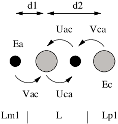
For further simplification, the transverse band structure is approximated by an isotropic parabolic dispersion, with the electronic effective mass replaced by the hole effective mass in the case of the valence band. What remains in the direction of propagation is a model with , which is equivalent to a linear chain of atoms, with the anion layers at the cation layers at , where labels the monolayer of thickness , with the lattice constant of the binary compound (i.e. 5.65 in the case of GaAs). In terms of the parameters introduced above, the elements of the TB-Hamiltonian
| (47) |
including parabolic transverse energy, are given by
| (48) | ||||
| (49) |
where is the effective electron and hole mass, respectively. This yields the bulk Hamiltonian
| (50) |
which for gives rise to the dispersion relation
| (51) |
For the integration over transverse momentum, the isotropic one dimensional approximation
| (52) |
is used, where is the device cross section, is the projected Brillouin zone and is the absolute value of the transverse momentum.
The tight-binding parameters are related to the longitudinal effective mass through the longitudinal dispersion relation, as , with resulting from the secular equation
| (53) |
From Eq. (51), one finds the relation between the effective mass at the -point and the coupling element ,
| (54) |
where is the energy gap.
Appendix B Boundary self energies for multiband tight-binding transport models
To properly model the effect of semi-infinite bulk at the lead-device interface, the interface Green’s function has to be linked to the propagating and evanescent states in the leads. The total electron wave function expressed in terms of the Bloch sum of the anion (a) and cation (c) states as a linear combination of planar orbitals is given by Eq. (3). In the planar orbital basis, projecting onto the atomic orbitals located at layer L, the Schrödinger equation for the contact Bloch states reads
| (55) | ||||
| (56) |
For a tight-binding Hamiltonian coupling neighboring layers, which is of the form
| (57) |
where represents a matrix which couples a given layer to the -th neighboring layer and is the layer spacing, and defining
| (58) |
Eq.(56) can be written as
| (59) |
where it was used that .
For a nearest neighbor Hamiltonian (), the projected Schrödinger
equation is recast into
| (60) |
which, using , can be written as
| (61) |
This equation can then be transformed into an eigenequation for the propagation factors and the lead Bloch states in local orbital basis:
| (62) |
with and , where and are the atomic layer transfer matrices defined as
| (63) |
with the matrix elements given by ( denotes the atomic layer)
| (64) | ||||
| (65) | ||||
| (66) |
The eigenstates and eigenvalues of Eq. (62) correspond to the bulk modes propagating (real ) or decaying (complex ) to the left () and to the right (), respectively. For an -band model with a two atom basis, there are states propagating or decaying to the right and to the left , respectively. At a given layer , the components for left- and right travelling waves can be written as
| (67) |
where is a vector containing the expansion coefficients, and
| (68) |
The corresponding expression for the adjacent layer is
| (69) |
with the propagation matrix
| (70) |
The relation between the two layers follows as
| (71) |
with
| (72) |
Relation (71) can be used to derive the retarded Green’s function at the right boundary () of the uncoupled semi infinite left lead, i.e. for the case where all the couplings to the right are set to zero. The equation
| (73) |
yields for the boundary element
| (74) |
Eq. (71) provides the relation
| (75) |
which determines the left lead boundary Green’s function in terms of the bulk modes as
| (76) | ||||
| (77) |
and providing thus an expression for the (left) retarded boundary self energy .
References
- (1) K. Barnham and G. Duggan, J. Appl. Phys. 67, 3490 (1990).
- (2) K. Barnham et al., Physica E 14, 27 (2002).
- (3) L. P. Kadanoff and G. Baym, Quantum Statistical Mechanics, Benjamin-Cummings, 1995.
- (4) L. Keldysh, Sov. Phys.-JETP. 20, 1018 (1965).
- (5) A. Wacker, Physics Reports 357, 1 (2002).
- (6) S.-C. Lee and A. Wacker, Phys. Rev. B 66, 245314 (2002).
- (7) L. E. Henrickson, J. Appl. Phys 91, 6273 (2002).
- (8) D. A. Stewart and F. Leonard, Phys. Rev. Lett. 93, 107401 (2004).
- (9) J. Guo, M. A. Alam, and Y. Yoon, Appl. Phys. Lett. 88, 133111 (2006).
- (10) R. Lake, G. Klimeck, R. Bowen, and D. Jovanovic, J. Appl. Phys. 81, 7845 (1997).
- (11) Y.-C. Chang and J. Schulman, Phys. Rev. B 25, 3975 (1981).
- (12) P. Vogl, H. Hjalmarson, and J. Dow, J. Phys. Chem. Solids 44, 365 (1983).
- (13) L. Lew Yan Voon and L. Ram-Mohan, Phys. Rev. B 47, 15500 (1993).
- (14) M. Graf and P. Vogl, Phys. Rev. B 51, 4940 (1995).
- (15) T. B. Boykin and P. Vogl, Phys. Rev. B 65, 035202 (2001).
- (16) C. Caroli, R. Combescot, P. Nozières, and D. Saint-James, J. Phys. C: Solid St. Phys. 4, 916 (1971).
- (17) S. Datta, Electronic Transport in Mesoscopic Systems, Cambridge University Press, 1995.
- (18) S. Sanvito, J. Lambert, J. Jefferson, and A. Bratkovsky, Phys. Rev. B 59, 11936 (1999).
- (19) C. Lent and D. Kirkner, J. Appl. Phys. 67, 6353 (1990).
- (20) T. Ando, Phys. Rev. B 44, 8017 (1991).
- (21) M. Ogawa, T. Sugano, R. Tominaga, and T. Miyoshi, Physica B 272, 167 (1999).
- (22) Bouwen, Phys. Rev. B 52, 2754 (1995).
- (23) P. Hyldgaard, S. Hershfield, J. Davies, and J. Wilkins, Ann. of Phys. 236, 1 (1994).
- (24) R. K. Lake and R. R. Pandey, arXiv:cond-mat/0607219v1 [cond-mat.mes-hall] (2006).
- (25) E. V. Anda and F. Flores, J. Phys., Condens. Matter. 3, 9087 (1991).
- (26) A. MacKinnon, Z. Phys. B - Condensed Matter 59, 385 (1985).
- (27) S. V. Faleev and M. I. Stockman, Phys. Rev. B 66, 085318 (2002).
- (28) T. B. Boykin, Phys. Rev. B 54, 7670 (1996).