Superfrustration of charge degrees of freedomThanks: Contribution to the proceedings of the XXIII IUPAP International Conference on Statistical Physics in Genova, Italy.
Abstract
We review recent results, obtained with P. Fendley, on frustration of quantum charges in lattice models for itinerant fermions with strong repulsive interactions. A judicious tuning of kinetic and interaction terms leads to models possessing supersymmetry. In such models frustration takes the form of what we call superfrustration: an extensive degeneracy of supersymmetric ground states. We present a gallery of examples of superfrustration on a variety of 2D lattices.
pacs
05.30.-dQuantum statistical mechanics and 11.30.PbSupersymmetry and 71.27.+aStrongly correlated electron systems; heavy fermions1 Introduction
When charged particles, with repulsive interactions, are placed on a lattice one expects geometric frustration: depending on the lattice and the number of particles, there can be many configurations that realize the lowest possible interaction energy. Well-studied examples are charges on the triangular and checkerboard lattices (see early-frus for some early references). In general, including kinetic terms for the quantum charges lifts the degeneracies. Depending on details, this may give rise to novel phases of quantum matter with remarkable physical properties frus. The theoretical tools for studying these systems are limited: one typically relies on a strong coupling expansions and on numerics.
Recent work by P. Fendley and one of the authors FS has uncovered models for strongly interacting itinerant fermions which display a strong form of quantum charge frustration, which we call superfrustration. These models (defined on 2D or 3D lattices) have a large, exact ground state degeneracy in the presence of kinetic terms. Superfrustration thus arises due to a subtle interplay between kinetic terms and strong repulsive interactions.
The term ‘superfrustration’ has its origin in a key property used to identify the models and to study their properties, which is supersymmetry. Quite remarkably, the notion of supersymmetry, which was developed in the context of high energy physics, turns out to be a powerful tool in the analysis of strongly correlated itinerant fermions. This was first recognized in the context of 1D models FSdB; FNS. The extension to 2D and 3D then led to the discovery of the phenomenon of superfrustration.
In this review, we shall first explain (Sect. 2) how supersymmetry is put to work in lattice models of correlated fermions. We introduce some basic tools, such as the Witten index, make a connection to cohomology theory and discuss a model on a 1D chain. We then move to models on 2D lattices (Sect. 3), where we present a heuristic geometric intuition (3-rule) and discuss the methods employed in the analysis. In Sect. 4 we present a gallery of examples, each chosen such as to illuminate specific aspects and features. They firmly establish the notion of superfrustration in its various guises. We close (Sect. 5) with some thoughts about the nature of the various ground states and quantum phases, in particular in relation to quantum criticality.
2 Supersymmetry
2.1 Basic algebra and Hamiltonian
In quantum mechanics, supersymmetric theories are characterized by a positive definite energy spectrum and a twofold degeneracy of each non-zero energy level. The two states with the same energy are called superpartners and are related by the nilpotent supercharge operator. Let us consider an supersymmetric theory, defined by two nilpotent supercharges and Wi,
and the Hamiltonian given by
From this definition it follows directly that is positive definite:
Furthermore, both and commute with the Hamiltonian, which gives rise to the twofold degeneracy in the energy spectrum. In other words, all eigenstates with an energy form doublet representations of the supersymmetry algebra. A doublet consists of two states , such that . Finally, all states with zero energy must be singlets: and conversely, all singlets must be zero energy states Wi. In addition to supersymmetry our models also have a fermion-number symmetry generated by the operator with
Consequently, commutes with the Hamiltonian.
The supersymmetric theories that we discuss in this paper describe fermionic particles. One might expect that, in order to be supersymmetric, these theories would need bosonic particles as well but this is not the case. The crux is that the quantum states in these theories come in two types: bosonic states, having an even number of fermionic particles, and fermionic states with odd. From the commutators of with the supercharges, one finds that and change by plus or minus one one unit, so that the supercharges map bosonic states to fermionic states and vice versa.
We now make things concrete and define supersymmetric models for spin-less fermions on a lattice or graph with sites in any dimension, following FSdB). The operator that creates a fermion on site is written as with . A simple choice for the first supercharge would be , where the sum is over all lattice sites. This leads to a trivial Hamiltonian: , where is the number of lattice sites. To obtain a non-trivial Hamiltonian, we dress the fermion with a projection operator: , which requires all sites adjacent to site to be empty. With and , the Hamiltonian of these hard-core fermions reads
The first term is just a nearest neighbor hopping term for hard-core fermions, the second term contains a next-nearest neighbor repulsion, a chemical potential and a constant. The details of the latter terms will depend on the lattice we choose.
Note that all the parameters in the Hamiltonian (the hopping , the nearest neighbor repulsion , the next-nearest neighbor repulsion and the chemical potential ) are fixed by the choice of the supercharges and the requirement of supersymmetry and eventually the lattice.
2.2 Witten index
We have already discussed how supersymmetry gives rise to certain properties of the spectrum of the system, such as positivity of the energies and pairing of the excited states. An important issue is whether or not supersymmetric ground states at zero energy occur. For this one considers the Witten index
| (1) |
Remember that all excited states come in doublets with the same energy and differing in their fermion-number by one. This means that in the trace all contributions of excited states will cancel pairwise, and that the only states contributing are the zero energy ground states. We can thus evaluate in the limit of , where all states contribute . It also follows that is a lower bound to the number of zero energy ground states.
2.3 Example: 6-site chain
Let us consider as an example of all the above, the chain of six sites with periodic boundary conditions. The first thing we note is that the Hamiltonian for an -site chain with periodic boundary conditions can be rewritten in the following form:
| (2) |
where
Here , is the usual number operator and is the total number of fermions. (We shall denote eigenvalues of this operator by and write the fermion density or filling fraction as .) The form of the hamiltonian makes clear that the hopping parameter is tuned to be equal to the next-nearest neighbor repulsion , which is tuned to unity. The nearest neighbor repulsion is by definition infinite and the chemical potential is . Finally, there is a constant contribution to the Hamiltonian. Note that the second term in the Hamiltonian suggests that the energy is minimized when the hard-core fermions are three sites apart.
Let us consider the possible configurations of the 6-site chain. In addition to the empty state, there are six configurations with one fermion, nine with two fermions and two with three fermions (see Fig. 1). Because of the hard-core character of the fermions, half-filling is the maximal density. Clearly, the operator gives zero on these maximally filled states. On the other hand, acts non-trivially on these states, so two of the nine states with two fermions are superpartners of the maximally filled states. The empty state has an energy and , whereas , so make up a doublet. The other five states with one fermion are annihilated by and acts non-trivially on them, so they form supersymmetry doublets with five two-fermion-states. At this point, seven of the nine two-fermion-states are paired up in doublets, either with one- or three-fermion-states. The remaining two states cannot be part of a doublet, which implies that they must be singlet states and thus have zero energy. So we find that the 6-site chain has a twofold degenerate zero energy ground state at filling . The full spectrum of the 6-site chain is shown in Fig. 1.
We observe that the ground state filling fraction of agrees with the expectation that fermions tend to be three sites apart. This geometric rule suggests three possible ground states; in the full quantum theory two are realized as zero-energy states. Note that the actual ground state wavefunctions are superpositions of many different configurations. With a bit more work one can show that the ground states have eigenvalues under translation by one site.

Now let us compute the Witten index for this example. Remember that for a supersymmetric theory it simply reads
Note that we can take any basis of states we like to compute the trace. Above we have specified a basis by considering all the possible configurations of up to three fermions on the chain. It immediately gives in agreement with the existence of the two ground states that we found.
We close this section with two comments. First, we stress that the extremely simple computation of alone guarantees the existence of at least two ground states at zero energy. Similar results are easily established for much larger systems, where a direct evaluation of the ground state energies is way out of reach, showing the power of supersymmetry. Second, we observe that here the Witten index is exactly equal to the number of ground states. We will encounter examples where ground states exist at more than one fermion number , leading to cancellations in the Witten index so that is strictly smaller than the number of ground states.
2.4 Cohomology
Supersymmetry supplies us with another tool, besides the Witten index, to study the ground states of the fermion models. This so-called cohomology method is more involved but it reveals more information about the ground state structure, in that it specifies the number of ground states for given fermion number .
The key ingredient is the fact that ground states are singlets, they are annihilated both by and . This means that a ground state is in the kernel of : . Such a ground state is not in the image of , because if we could write , then , would be a doublet. Equivalently, we can say that a ground state is closed but not exact. So the ground states span a subspace of the Hilbert space of states, such that . This is precisely the definition of the cohomology of . So the ground states of a supersymmetric theory are in one-to-one correspondence with the cohomology of . Two states and are said to be in the same cohomology-class if for some state . Since a ground state is annihilated by both and , different (i.e. linearly independent) ground states must be in different cohomology-classes of . Finally, the number of independent ground states is precisely the dimension of the cohomology of and the fermion-number of a ground state is the same as that of the corresponding cohomology-class.
There are several techniques to compute the cohomology, which we shall illustrate by working out examples in the following sections.
2.5 Example: 1D chains
In previous work FS; FSdB; FNS; BDA the supersymmetric model on the chain was studied extensively. We will summarize some of the results, but mostly use this case to illustrate the power of the tools we have developed in the previous sections. Let us first compute the Witten index. In the example of the 6-site chain we saw that the Witten index can be computed by simply summing over all possible configurations with the appropriate sign. However, because of the hard-core character of the fermions this is not a trivial problem for larger sizes. Here we shall exploit a much more elegant method, which will turn out very useful when we extend our model to more complex lattices. This method consists of the following steps: first divide the lattice into two sublattices and . Then fix the configuration on and sum for the configurations on . Finally, sum the results over the configurations of . Of course the trick is to make a smart choice for the sublattices. For the periodic chain with sites, we take to be every third site. All the sites on are disconnected and thus every site can be either empty or occupied given that its neighboring sites on are empty. This means that the sum of for the configurations on vanishes as soon as at least one site on can be both empty and occupied. Consequently, the only non-zero contribution comes from the configurations such that at least one of the adjacent sites on is occupied. There are only two such configurations:
| (3) |
where the square represents an empty site on . The final step is to sum for these two configurations, and since both configurations have , we find that the Witten index is . Note that this agrees with the result we obtained for the 6-site chain.
To find the exact number of ground states we compute the cohomology by using a spectral sequence. A useful theorem is the ‘tic-tac-toe’ lemma of BT. This says that under certain conditions, the cohomology for is the same as the cohomology of acting on the cohomology of . In an equation, , where and act on different sublattices and . We find by first fixing the configuration on all sites of the sublattice , and computing the cohomology . Then one computes the cohomology of , acting not on the full space of states, but only on the classes in . A sufficient condition for the lemma to hold is that all non-trivial elements of have the same (the fermion-number on ). For the periodic chain with we choose the sublattice as before. Now consider a single site on . If both of the adjacent sites are empty, is trivial: acting on the empty site does not vanish, while the filled site is acting on the empty site. Thus is non-trivial only when every site on is forced to be empty by being adjacent to an occupied site. The elements of are just the two states and pictured above in eq. (2.5). Both states and belong to : they are closed because , and not exact because there are no elements of with . By the tic-tac-toe lemma, there must be precisely two different cohomology classes in , and therefore exactly two ground states with . Applying the same arguments to the periodic chain with sites and to the open chain yields in all cases exactly one ground state, except in open chains with sites, where there are none FNS.
The supersymmetric model on the chain can be solved exactly through a Bethe Ansatz FSdB. In the continuum limit one can derive the thermodynamic Bethe ansatz equations. The model has the same thermodynamic equations as the XXZ chain at , so the two models coincide (the mapping can be found in FNS). The continuum limit of the XXZ chain is described by the massless Thirring model hank, or equivalently a free massless boson with action Friedan
The continuum limit of the model has ; this is the simplest field theory with superconformal symmetry Friedan. The means that there are two left and two right-moving supersymmetries: in the continuum limit the fermion decomposes into left- and right-moving components over the Fermi sea. So the system is critical and in the continuum limit it is described by a superconformal field theory.
A final note we would like to make here, is that the supersymmetric model on the chain recently emerged in a special limit of a large- supersymmetric matrix model VW. This is yet another interesting connection, worthy of further investigation.
3 Beyond 1D: heuristics and methodology
We have seen that in the one dimensional case the Hamiltonian favors a configuration where the hard-core fermions sit three sites apart on average. This heuristic picture can be extended beyond 1D. For convenience we restate the Hamiltonian in its general form
The second term in the Hamiltonian gives a positive contribution to the energy for every site that has all neighboring sites empty, regardless of whether the site itself is occupied or empty. For every hard-core fermion it will give a contribution of , since by definition it has its neighboring sites empty. So the contribution of this term is minimized by blocking as many sites as possible with as few fermions as possible. Roughly speaking, this criterion leads to configurations where all fermions are three sites apart. We call this the ‘3-rule’. In the following sections we shall see this 3-rule in action, and demonstrate how it leads to superfrustration.
In the previous section we have developed some tools to study our model on different lattices. The Witten index gives us a lower bound on the total number of supersymmetric ground states. In some cases one can find a recursion relation or even a closed form for the Witten index as a function of the system size. The growth behavior of this function gives a lower bound to the growth behavior of the ground state entropy.
If the Witten index grows exponentially with the system size, we have an extensive ground state entropy. In Sect. 4.1 we present an example where this entropy is known in closed form. Numerical studies of the Witten index on two-dimensional lattices vE have revealed that for generic lattices the Witten index indeed grows exponentially with the system size (see Sect. 4.3 for an example). The square lattice is an exception, since there the Witten index grows exponentially with the perimeter of the system. We shall touch upon some features of the square lattice in Sect. 4.4.
Further insight in the ground state structure can be obtained from the cohomology method. This gives the exact number of ground states and for each of them the number of fermions. A remarkable feature of our model that has been revealed by cohomology studies is that ground states typically occur at different fermion-numbers, or equivalently at different filling fractions. This implies that the Witten index will typically underestimate the actual number of ground states. More remarkably, however, this also implies that one can add a particle to the system or extract a particle from the system within a certain window of filling fractions without paying any energy.
Finally, it has in many cases turned out to be possible to characterize supersymmetric ground states with the help of an ‘effective geometric picture’. In this, one establishes a (almost) 1-1 correspondence between quantum ground states and geometric configurations such as coverings of the lattice by dimers or tiles of specific dimensions. Examples are dimer coverings for the case of the martini lattice (Sect. 4.1) and rhombus tilings for the 2D square lattice (Sect. 4.4). The geometric picture is related to the heuristic 3-rule, but much more robust. It has been pioneered in FS and in a remarkable series of mathematical papers by J. Jonsson Jo.
The fact that the ground states of strongly correlated quantum fermion models can be characterized by geometric means is quite deep and at this time not fully understood. It suggests that further properties of these models (such as the excited state spectra) are tractable by similar means, which opens most interesting perspectives.
It the next section we present a gallery of examples of 2D lattices, and indicate what has been revealed about their ground state structure using the various approaches described in this section. A more systematic account is forthcoming FHHS.
4 Beyond 1D: examples
4.1 Martini lattice
The martini lattice (see Fig. 2) is an example of a two dimensional lattice, where the cohomology can be computed relatively easily FS. The method is strongly related to the one used to compute the cohomology for the chain. The computation proves that the ground state entropy is an extensive quantity and we find a closed expression for the ground state entropy per site. We shall see that the 3-rule is not violated in this case. This is related to the fact that the martini lattice, due to its structure, nicely accommodates the 3-rule. Lattices with a higher coordination number usually do not have this property and consequently allow for a window of filling fraction for the supersymmetric ground states.
The martini lattice is formed by replacing every other site on a hexagonal lattice with a triangle. To find the ground states, take to be the sites on the triangles, and to be the remaining sites. As with the chain, vanishes unless every site in is adjacent to an occupied site on some triangle. The non-trivial elements of therefore must have precisely one particle per triangle, each adjacent to a different site on . This is because a triangle can have at most one particle on it, and (with appropriate boundary conditions) there are the same number of triangles as there are sites on . A typical element of is shown in Fig. 2. One can think of these as ‘dimer’ configurations on the original honeycomb lattice, where the dimer stretches from the site replaced by the triangle to the adjacent non-triangle site. Each close-packed hard-core dimer configuration is in , and by the tic-tac-toe lemma, it corresponds to a ground state. The number of such ground states is therefore equal to the number of such dimer coverings of the honeycomb lattice, which for large is dimer
The frustration here clearly arises because there are many ways of satisfying the 3-rule.

4.2 Kagome ladder
In this section we consider the kagome ladder (see Fig. 2) as an illustration of a case where we can compute the cohomology exactly, but where the 3-rule is not very helpful. We find a closed expression for the partition function and a window of filling fraction for the supersymmetric ground states, which can both be interpreted in terms of tilings.
Computing the cohomology in this case is a bit more involved due to two things: First, in the previous examples we could always choose the sublattice such that it consisted of disconnected sites, which by themselves have zero cohomology. For the kagome ladder the convenient choice for the sublattice is less trivial. The second complication arises because not all elements of the cohomology will have the same fermion-number, which was a sufficient condition for the tic-tac-toe lemma to hold.

We compute the cohomology step by step. For each step there is a supporting picture in Fig. 3. Step 1 is to map the kagome ladder with hard-core fermions to a square ladder with hard-core dimers. This mapping is one-on-one. In Step 2 we define the sublattices and . Step 3 is to note that the cohomology of one square plus one additional edge vanishes. To do so, first note that if site 3 and 4 are both empty, we get zero cohomology due to site 5 which can now be both empty and occupied. The remaining four configurations are easily shown to be either of something (exact) or not in the kernel of (not closed). Step 4 is to build up the ladder by consecutively adding blocks with 3 rungs (9 edges) to the ladder. From step 3 we now conclude that there are only two allowed configurations for the additional -sites: they must be either both empty or both occupied, since if just one of them is occupied the remaining configurations on the additional -sites are exactly the ones of step 3. A simple computation shows that if both sites on are occupied, has one non-trivial element with one dimer and if both sites on are empty, has two non-trivial elements, both with two dimers.
Now it is important to note that on the three additional rungs we find three non-trivial elements of the , but two of them have and one has . It can be shown that all three indeed belong to by going through the tic-tac-toe lemma step by step. This is a tedious computation, but it can be done.
Finally, we find the cohomology of the kagome ladder with open boundary conditions of length , which corresponds to a ladder with rungs and edges in total, by recursively adding rungs to the system. We thus obtain a recursion relation for the ground-state generating function , which gives the Witten index for and the total number of ground states for :
with , , , . Instead of drawing conclusion from here, let us picture the above in terms of tiles. From step 4 we conclude that we can cover the ladder with three tiles, two of size 9 (i.e. 9 edges) containing 2 dimers and one of size 12 containing 3 dimers. From this picture we obtain the same recursion relation provided that we allow four initial tiles corresponding to the initial conditions of the recursion relation above. Furthermore, we can see directly that the window of filling fraction of the tiles runs from 2/9 to 1/4. Using the recursion relation, we find that the ground-state entropy is set by the largest solution of the characteristic polynomial , giving .
4.3 2D triangular lattice
The ground state structure of the supersymmetric model on the 2D triangular lattice is not fully understood. Nevertheless, it is clear that ground states occur in a finite window of filling fractions and that there is extensive ground state entropy. These features seem to be generic for 2D lattices, as they have been observed for many examples such as hexagonal, kagome, etc. (2D square being an important exception) vE.
| 1 | 2 | 3 | 4 | 5 | 6 | 7 | |
| 1 | 1 | 1 | 1 | 1 | 1 | 1 | 1 |
| 2 | 1 | -3 | -5 | 1 | 11 | 9 | -13 |
| 3 | 1 | -5 | -2 | 7 | 1 | -14 | 1 |
| 4 | 1 | 1 | 7 | -23 | 11 | 25 | -69 |
| 5 | 1 | 11 | 1 | 11 | 36 | -49 | 211 |
| 6 | 1 | 9 | -14 | 25 | -49 | -102 | -13 |
| 7 | 1 | -13 | 1 | -69 | 211 | -13 | -797 |
| 8 | 1 | -31 | 31 | 193 | -349 | -415 | 3403 |
| 9 | 1 | -5 | -2 | -29 | 881 | 1462 | -7055 |
| 10 | 1 | 57 | -65 | -279 | -1064 | -4911 | 5237 |
| 11 | 1 | 67 | 1 | 859 | 1651 | 12607 | 32418 |
| 12 | 1 | -47 | 130 | -1295 | -589 | -26006 | -152697 |
| 13 | 1 | -181 | 1 | -77 | -1949 | 67523 | 330331 |
| 14 | 1 | -87 | -257 | 3641 | 12611 | -139935 | -235717 |
| 15 | 1 | 275 | -2 | -8053 | -32664 | 272486 | -1184714 |
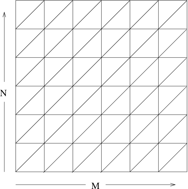
In Tab. 1 we show the Witten indices for the triangular lattice, with periodic boundary conditions applied along two axes of the lattice (see Fig. 4). The exponential growth of the index is clear from the table. To quantify the growth behavior, one may determine the largest eigenvalue of the row-to-row transfer matrix for the Witten index on size . This gives
| (4) |
leading to a ground state entropy per site of
| (5) |
The argument of indicates that the asymptotic behavior of the index is dominated by configurations with filling fraction around .
In a most interesting mathematical analysis Jo, Jonsson has shown that for a sufficiently large triangular lattice (with open BC) ground states occur for all rational numbers in the range
| (6) |
His analysis is based on an effective geometric picture involving so-called cross-cycles, which however is less explicit than the one that has been worked out for the case of the 2D square lattice (see below). There is a clear challenge to develop this picture further to the point that the growth behavior of the Witten index, and of the number of ground states, can be given in closed form.
4.4 2D square lattice
| 1 | 2 | 3 | 4 | 5 | 6 | 7 | 8 | 9 | 10 | 11 | 12 | |
|---|---|---|---|---|---|---|---|---|---|---|---|---|
| 1 | 1 | 1 | 1 | 1 | 1 | 1 | 1 | 1 | 1 | 1 | 1 | 1 |
| 2 | 1 | -1 | 1 | 3 | 1 | -1 | 1 | 3 | 1 | -1 | 1 | 3 |
| 3 | 1 | 1 | 4 | 1 | 1 | 4 | 1 | 1 | 4 | 1 | 1 | 4 |
| 4 | 1 | 3 | 1 | 7 | 1 | 3 | 1 | 7 | 1 | 3 | 1 | 7 |
| 5 | 1 | 1 | 1 | 1 | -9 | 1 | 1 | 1 | 1 | 11 | 1 | 1 |
| 6 | 1 | -1 | 4 | 3 | 1 | 14 | 1 | 3 | 4 | -1 | 1 | 18 |
| 7 | 1 | 1 | 1 | 1 | 1 | 1 | 1 | 1 | 1 | 1 | 1 | 1 |
| 8 | 1 | 3 | 1 | 7 | 1 | 3 | 1 | 7 | 1 | 43 | 1 | 7 |
| 9 | 1 | 1 | 4 | 1 | 1 | 4 | 1 | 1 | 40 | 1 | 1 | 4 |
| 10 | 1 | -1 | 1 | 3 | 11 | -1 | 1 | 43 | 1 | 9 | 1 | 3 |
| 11 | 1 | 1 | 1 | 1 | 1 | 1 | 1 | 1 | 1 | 1 | 1 | 1 |
| 12 | 1 | 3 | 4 | 7 | 1 | 18 | 1 | 7 | 4 | 3 | 1 | 166 |
| 13 | 1 | 1 | 1 | 1 | 1 | 1 | 1 | 1 | 1 | 1 | 1 | 1 |
| 14 | 1 | -1 | 1 | 3 | 1 | -1 | -27 | 3 | 1 | 69 | 1 | 3 |
| 15 | 1 | 1 | 4 | 1 | -9 | 4 | 1 | 1 | 4 | 11 | 1 | 4 |
Numerical studies FSvE of the Witten index of the square lattice revealed a very different behavior (see Tab. 2). At first glance one notices that it does not grow exponentially with the system size. In fact, more detailed investigation of these studies led to two conjectures FSvE for which a proof was found by Jonsson Jo. We state one of these results here:
for an square lattice with periodic boundary conditions in both directions, when and are coprime.
Extending this work, Jonsson found a general expression for the Witten index of hard-core fermions on the square lattice with periodic boundary conditions given by the vectors and . The square lattice is now a specific case with and (for an extension of this work to other families of grid graphs see BMLN). A crucial step in Jo is the introduction of rhombus tilings of the square lattice. It is shown that the trace in the Witten index can be restricted to configurations that can be mapped to coverings of the plane with the four rhombi or tiles shown in Fig. 5.

Note that the sides of these rhombi, which connect the hard-core fermions, are in agreement with the heuristic 3-rule. Furthermore, two of the rhombi have area 4, whereas the other two have area 5. A covering with either of these rhombi alone thus corresponds to a filling fraction of 1/4 or 1/5, respectively.
To state Jonsson’s results for the Witten index we introduce the following notations. We denote by the family of tilings of the plane with boundary conditions given by and . Furthermore and are the number of tilings of this plane with an even and an odd number of tiles, respectively. Finally, we define
| (7) |
The expression for the Witten index then reads Jo
| (8) |
where and . It can be shown that the Witten index grows exponentially with the linear size (not the area) of the 2D lattice. Detailed results for the case of diagonal boundary conditions have been given in Jo2. Further studies of the Witten index transfermatrix for the square lattice with diagonal and free boundary conditions by R.J. Baxter RJB have led to an additional set of conjectures.
As we already mentioned in Sect. 3, the geometric picture in terms of tilings is useful beyond the computation of the Witten index. It also provides a way to determine a window of filling fractions in which supersymmetric ground states can be found. The result is Jo that for large enough square lattices (with open BC) ground states exist for all rational fillings in the range
| (9) |
While it is clear that the effective geometric picture in terms of rhombus tilings goes a long way characterizing the supersymmetric ground states, it has until now failed to give complete results for the ground state partition sum for the supersymmetric model on the 2D square lattice. For this issue, and for many others, it is important that the results presented in this section hold for the square lattice with any kind of periodic boundary conditions. This also includes semi-2D lattices, i.e. various ladders and even the 1D chain. These lattices are a good arena to further investigate properties of the supersymmetric fermion models, both analytically and numerically FHHS.
5 Conclusion
The analysis of strongly correlated fermions on lattices in dimension is a notoriously difficult problem, for which very few exact results have been obtained. At the same time, the problem is highly relevant, as it holds the key to the behavior of correlated electrons in quasi-2D materials. We have here presented various exact results for the ground state structure of a fermion lattice model with an exact supersymmetry. In particular, we have demonstrated the remarkable feature of superfrustration, which this model possesses on generic 2D lattices.
In our discussion of the various examples of superfrustration, we mostly focused on specifying the number of supersymmetric ground states and the fermion number (or filling fraction) where they occur. Clearly, one would like to understand better various properties of these states, as well as the quantum phases they give rise to when parameters are perturbed away from the supersymmetric point.
The supersymmetric ground states on the 1D chain are quantum critical and as such described by a superconformal field theory. For a more general class of supersymmetric 1D models FNS (where the nearest neighbor exclusion rule is softened) the situation is akin to that of higher- spin chains: the models are gapped but go critical if interaction parameters are tuned to specific values. For the 2D models presented here, the issue of quantum criticality is under investigation FHHS. While supersymmetry alone certainly does not imply quantum criticality, it is clear that the balancing between kinetic and interaction terms that is implied by supersymmetry steers one into regions of parameter space where charge order and Fermi liquid behavior compete.
Acknowledgements. We thank Paul Fendley and Hendrik van Eerten for collaboration on the research that is here reviewed. We acknowledge financial support through a PIONIER grant of NWO of the Netherlands and through the Research Networking Programme INSTANS of the ESF.
References
- (1) E.J.W. Verwey, Nature (London) 144, 327 (1939); P.W. Anderson, Phys. Rev. 102, 1008 (1956); G.H. Wannier, Phys. Rev. 79, 357 (1950).
- (2) E. Runge and P. Fulde, Phys. Rev. B70, 245113 (2004); O.I. Motrunich and P.A. Lee, Phys. Rev. B69, 214516 (2004).
- (3) P. Fendley, K. Schoutens, Phys. Rev. Lett. 95, 046403 (2005) [arXiv:hep-th/0504595].
- (4) P. Fendley, K. Schoutens, and J. de Boer, Phys. Rev. Lett. 90, 120402 (2003) [arXiv:hep-th/0210161].
- (5) P. Fendley, B. Nienhuis and K. Schoutens, J. Phys. A 36, 12399 (2003) [arXiv:cond-mat/0307338].
- (6) E. Witten, Nucl. Phys. B202 (1982) 253.
- (7) M. Beccaria and G. F. De Angelis, Phys. Rev. Lett. 94, 100401 (2005) [arXiv:cond-mat/0407752].
- (8) R. Bott and L.W. Tu, Differential Forms in Algebraic Topology, GTM 82, (Springer Verlag, New York, 1982).
- (9) H. B. Thacker, Rev. Mod. Phys. 53 (1981) 253.
- (10) D. Friedan and S. H. Shenker, in C. Itzykson, H. Saleur and J.B. Zuber, Conformal invariance and applications to statistical mechanics (World Scientific, 1988).
- (11) G. Veneziano and J. Wosiek, JHEP 0611 (2006) 030 [arXiv:hep-th/0609210]
- (12) H. van Eerten, J. Math. Phys. 46, 123302 (2005) [arXiv:cond-mat/0509581].
- (13) J. Jonsson, Electronic Journal of Combinatorics 13(1), #R67 (2006); Certain Homology Cycles of the Independence Complex of Grid Graphs, Preprint (October 2005).
- (14) P. Fendley, J. Halverson, L. Huijse and K. Schoutens, manuscript in preparation.
- (15) P.W. Kasteleyn, J. Math. Phys. 4, 287 (1963); F.Y. Wu, Phys. Rev. 168, 539 (1967).
- (16) P. Fendley, K. Schoutens and H. van Eerten, J. Phys. A 38, 315 (2005) [arXiv:cond-mat/0408497].
- (17) M. Bousquet-Melou, S. Linusson and E. Nevo, On the independence complex of square grids, Preprint (2007) [arXiv:math/0701890].
- (18) J. Jonsson, Hard Squares on Grids With Diagonal Boundary Conditions, Preprint (August 2006).
- (19) R.J. Baxter, Hard squares for , preprint in preparation.