Flexible least squares for temporal data mining
and statistical arbitrage

Opportunities for pairs trading in the simple form described above are dependent upon the existence of similar pairs of assets, and thus are naturally limited. Many other variations and extensions exist that exploit temporary mispricing among securities. For instance, in index arbitrage, the investor looks for temporary discrepancies between the prices of the stocks comprising an index and the price of a futures contract²² 2 A futures contract is an obligation to buy or sell a certain underlying instrument at a specific date and price, in the future.on that index. By buying either the stocks or the futures contract and selling the other, market inefficiency can be exploited for a profit.

In this paper we adopt a simpler strategy than index arbitrage, somewhat more related to pairs trading. The trading system we develop tries to exploit discrepancies between a target asset, selected by the investor, and a paired artificial asset that reproduces the target asset. This artificial asset is represented by a data stream obtained as a linear combination of a possibly large set of explanatory streams assumed to be correlated with the target stream.

The rationale behind this approach is the following: if there is a strong association between synthetic and target assets persisting over a long period of time, this association implies that both assets react to some underlying (and unobserved) systematic component of risk that explains their dynamics. Such a systematic component may include all market-related sources of risk, including financial and economic factors. The objective of this approach is to neutralize all marker-related sources of risks and ultimately obtain a data stream that best represents the target-specific risk, also known as idiosyncratic risk.

Suppose that $y_{t}$ represents the data stream of the target asset, and $\widehat{y}_{t}$ is the artificial asset estimated using a set of $p$ explanatory and co-evolving data streams $x_{1},\ldots,x_{p}$, over the same time period. In this context, the artificial asset can also be interpreted as the fair price of the target asset, given all available information and market conditions. The difference $y_{t}-\widehat{y}_{t}$ then represents the risk associated with the target asset only, or mispricing. Given that this construction indirectly accounts for all sources of variations due to various market-related factors, the mispricing data stream is more likely to contain predictable patterns (such as the mean-reverting behavior seen in Figure 1) that could potentially be exploited for speculative purposes. For instance, in an analogy with the pairs trading approach, a possibly large mispricing (in absolute value) would flag a temporary inefficiency that will soon be corrected by the market. This construction crucially relies on accurately and dynamically estimating the artificial asset, and we discuss this problem next.

As noted above, the original FLS has been introduced for situations in which all the data points are available, in batch, prior to the analysis. In contrast, we are interested in situations where each data point arrives sequentially. Each component of the $p$ dimensional vector $x_{t}$ represents a new point of a data stream, and the path of regression coefficients needs to be updated at each time step so as to incorporate the most recently acquired information. Using the FLS machinery in this setting, the estimate of $\beta_{t}$ is given recursively by

where, by substituting $M_{t}$ and $d_{t}$ in (9) and (10), we obtain the recursions of $S_{t}$ and $s_{t}$ as

These recursions are initially started with some arbitrarily chosen values $S_{0}$ and $s_{0}$.

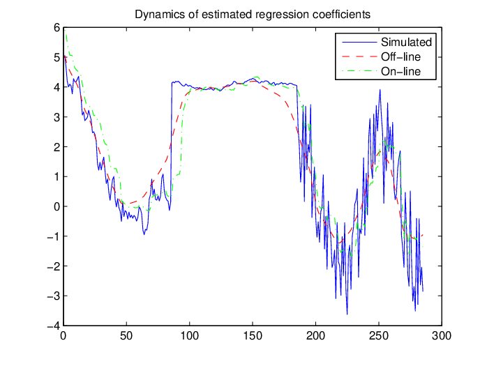
Figure 2 illustrates how accurately the FLS algorithm recovers the path of the time-varying coefficients, in both off-line and on-line settings, for some artificially created data streams. The target stream $y_{t}$ for this example has been generated using the model

where $\epsilon_{t}$ is uniformly distributed over the interval $[-2,2]$ and the explanatory stream $x_{t}$ evolves as

with $z_{t}$ being white noise. The regression coefficients have been generated using a slightly complex mechanism for the purpose of illustrating the flexibility of FLS. Starting with $\beta_{1}=7$, we then generate $\beta_{t}$ as

where $a_{t}$ and $b_{t}$ are Gaussian random variables with standard deviations $0.1$ and $0.001$, respectively, and $c_{t}$ is uniformly distributed over $[-2,2]$. We remark that this example features non-Gaussian error terms, as well as linear and non-linear behaviors in the dynamics of the regression coefficient, varying over time.

In this example we set $\delta=0.98$. Although such a high value of $\delta$ encourages the regression parameters to be very dynamic, the nearly constant coefficients observed between $t=101$ and $t=200$, as well as the two sudden jumps at times $t=100$ and $t=201$, are estimated well, and especially so in the on-line setting. The non-linear dynamics observed from time $t=201$ onwards is also well captured.

In our formulation, the regression coefficient at time $t+1$ is modeled as a noisy version of the previous coefficient at time $t$. First, we introduce a random vector $\omega_{t}$ with zero mean and some covariance matrix $V_{\omega}$, so that

Then, along the same lines, we introduce a random variable $\epsilon_{t}$ having zero mean and some variance $V_{\epsilon}$, so that

Equations (14) and (15), jointly considered, result in a linear state-space model, for which it is assumed that the innovation series $\{\epsilon_{t}\}$ and $\{\omega_{t}\}$ are mutually and individually uncorrelated, i.e. $\epsilon_{i}$ is uncorrelated of $\epsilon_{j}$, $\omega_{i}$ is uncorrelated of $\omega_{j}$, and $\epsilon_{k}$ is uncorrelated of $\omega_{\ell}$, for any $i\neq j$ and for any $k,\ell$. It is also assumed that for all $t$, $\epsilon_{t}$ and $\omega_{t}$ are uncorrelated of the initial state $\beta_{0}$. It should be emphasized again that no specific distribution assumptions for $\epsilon_{t}$ and $\omega_{t}$ have been made. We only assume that $\epsilon_{t}$ and $\omega_{t}$ attain some distributions, which we do not know. We only need to specify the first two moments of such distributions. In this sense, the only difference between the system specified by (14)-(15) and FLS is the assumption of randomness of $\beta_{t}$.

The Kalman filter (Kalman 1960) is a powerful method for the estimation of $\beta_{t}$ in the above linear state-space model. In order to establish the connection between FLS and KF, we derive an alternative and self-contained proof of the KF recursions that make no assumptions on the distributions of $\epsilon_{t}$ and $\omega_{t}$. We have found related proofs of such recursions that do not rely on probabilistic assumptions, as in Kalman 1960 and Eubank 2006. In comparison with these, we believe that our derivation is simpler and does not involve matrix inversions, which serves our purposes well.

We start with some definitions and notation. At time $t$, we denote by $\widehat{\beta}_{t}$ the estimate of $\beta_{t}$ and by $\widehat{y}_{t+1}=E(y_{t+1})$ the one-step forecast of $y_{t+1}$, where $E(.)$ denotes expectation. The variance of $y_{t+1}$ is known as the one-step forecast variance and is denoted by $Q_{t}=\text{Var}(y_{t+1})$. The one-step forecast error is defined as $e_{t}=y_{t}-E(y_{t})$. We also define the covariance matrix of $\beta_{t}-\widehat{\beta}_{t}$ as $P_{t}$ and the covariance matrix of $\beta_{t}-\widehat{\beta}_{t-1}$ as $R_{t}$ and we write $\text{Cov}(\beta_{t}-\widehat{\beta}_{t})=P_{t}$ and $\text{Cov}(\beta_{t}-\widehat{\beta}_{t-1})=R_{t}$. With these definitions, and assuming linearity of the system, we can see that, at time $t-1$

where $P_{t-1}$ and $\widehat{\beta}_{t-1}$ are assumed known. The KF gives recursive updating equations for $P_{t}$ and $\widehat{\beta}_{t}$ as functions of $P_{t-1}$ and $\widehat{\beta}_{t-1}$.

Suppose we wish to obtain an estimator of $\beta_{t}$ that is linear in $y_{t}$, that is $\widehat{\beta}_{t}=a_{t}+K_{t}y_{t}$, for some $a_{t}$ and $K_{t}$ (to be specified later). Then we can write

with $e_{t}=y_{t}-x_{t}^{\prime}\widehat{\beta}_{t-1}$. We will show that for some $K_{t}$, if $\widehat{\beta}_{t}$ is required to minimize the sum of squares

then $a_{t}^{*}=\widehat{\beta}_{t-1}$. To prove this, write $Y=(y_{1},\ldots,y_{T})^{\prime}$, $X=(x_{1}^{\prime},\ldots,x_{T}^{\prime})^{\prime}$, $B=(\beta_{1}^{\prime},\ldots,\beta_{T}^{\prime})^{\prime}$, $\mathcal{E}=(e_{1},\ldots,e_{T})^{\prime}$ and

Then we can write (17) as

and $\widehat{B}=A^{*}+K\mathcal{E}$, where $A^{*}=((a_{1}^{*})^{\prime},\ldots,(a_{T}^{*})^{\prime})^{\prime}$. We will show that $A^{*}=B^{*}$, where $B^{*}=(\widehat{\beta}_{0}^{\prime},\ldots,\widehat{\beta}_{T-1}^{\prime})^{\prime}$. With the above $\widehat{B}$, the sum of squares can be written as

which is minimized when $Y-XA^{*}$ is minimized or when $E(Y-XA^{*})=0$, leading to $A^{*}=B^{*}$ as required. Thus, $a_{t}^{*}=\widehat{\beta}_{t-1}$ and from (16) we have

for some value of $K_{t}$ to be defined. From the definition of $P_{t}$, we have that

Now, we can choose $K_{t}$ that minimizes

which is the same as minimizing the trace of $P_{t}$, and thus $K_{t}$ is the solution of the matrix equation

where $\partial\textrm{trace}(P_{t})/\partial K_{t}$ denotes the partial derivative of the trace of $P_{t}$ with respect to $K_{t}$. Solving the above equation we obtain $K_{t}=R_{t}x_{t}/Q_{t}$. The quantity $K_{t}$, also known as the Kalman gain, is optimal in the sense that among all linear estimators $\widehat{\beta}_{t}$, (18) minimizes $E(\beta_{t}-\widehat{\beta}_{t})^{\prime}(\beta_{t}-\widehat{\beta}_{t})$. With $K_{t}=R_{t}x_{t}/Q_{t}$, from (19) the minimum covariance matrix $P_{t}$ becomes

The KF consists of equations (18) and (20), together with

Initial values for $\widehat{\beta}_{0}$ and $P_{0}$ have to be placed; usually we set $\widehat{\beta}_{0}=0$ and $P_{0}^{-1}=0$.

Note that from the recursions of $P_{t}$ and $R_{t}$ we have

Traditionally, the KF equations are derived under the assumption that $\epsilon_{t}$ and $\omega_{t}$ follow the normal distribution, as in Jazwinski 1970. This stronger distributional assumption allows the derivation of the likelihood function. When the normal likelihood is available, we note that its maximization is equivalent to minimizing the quantity

with respect to $\beta_{1},\ldots,\beta_{T}$, where $\xi_{t}$ has been defined in (5) (see Jazwinski 1970 for a proof). The above expression is exactly the cost function (4) with $\mu$ replaced by $1/V_{\omega}$.

This correspondence can now be taken a step further: in a more general setting, where no distributional assumptions are made, it is possible to arrive to the same result. This is achieved by rearranging equation (11) in the form of (18), which is the KF estimator of $\beta_{t}$. First, note that from (12) we can write

and substituting to (11) we get $\widehat{\beta}_{t}=S_{t}^{-1}s_{t}$. Thus we have

with

It remains to prove that the recursion of $S_{t}$ as in (12) communicates with the recursion of (21), for $R_{t+1}=S_{t}^{-1}$. To end this, starting from (12) and using the matrix inversion lemma, we obtain

which is the KF recursion (21), where $V_{\omega}=\mu^{-1}I_{p}$.

Clearly, the FLS estimator $\widehat{\beta}_{t}$ of (11) is the same as the KF estimator $\widehat{\beta}_{t}$ of (18). From this equivalence, and in particular from $V_{\omega}=\mu^{-1}I_{p}$, it follows that

This result further clarifies the role of the smoothing parameter $\mu$ in (4). As $\mu\rightarrow\infty$, the covariance matrix of $\beta_{t+1}-\beta_{t}$ is almost zero, which means that $\beta_{t+1}=\beta_{t}$, for all $t$, reducing the model to a usual regression model with constant coefficients. In the other extreme, when $\mu\approx 0$, the covariance matrix of $\beta_{t+1}-\beta_{t}$ has very high diagonal elements (variances) and therefore the estimated $\beta_{t}$’s fluctuate erratically.

An important computational consequence of the established correspondence between the FLS and the KF is apparent. For each time $t$, FLS requires the inversion of two matrices, namely $S_{t-1}+x_{t}x_{t}^{\prime}$ and $S_{t-1}+\mu I_{p}+x_{t}x_{t}^{\prime}$. However, these inversions are not necessary, as it is clear by the KF that $\widehat{\beta}_{t}$ can be computed by performing only matrix multiplications. This is particulary useful for temporal data mining data applications when $T$ can be infinite and $p$ very large.

It is interesting to note how the two procedures arrive to the same solution, although they are based on quite different principles. On one hand, FLS merely solves an optimization problem, as it minimizes the cost function $C(\mu)$ of (4). On the other hand, KF performs two steps: first, all linear estimators are restricted to forms of (18), for any parameter vector $K_{t}$; in the second step, $K_{t}$ is optimized so that it minimizes $P_{t}$, the covariance matrix of $\beta_{t}-\widehat{\beta}_{t}$. This matrix, known as the error matrix of $\beta_{t}$, gives a measure of the uncertainty of the estimation of $\beta_{t}$.

The relationship between FLS and KF has important implications for both methods. For FLS, it suggests that the regression coefficients can be learned from the data in a recursive way without the need of performing matrix inversions; also, the error matrix $P_{t}$ is routinely available to us. For KF, we have proved that the estimator $\widehat{\beta}_{t}$ minimizes the cost function $C(\mu)=C(1/V_{\omega})$ when only the mean and the variance of the innovations $\epsilon_{t}$ and $\omega_{t}$ are specified, without assuming these errors to be normally distributed.

We have developed a statistical arbitrage system that trades S&P $500$ stock-index futures contracts. The underlying instrument in this case is the S&P $500$ Price Index, a world renowned index of $500$ US equities with minimum capitalization of $4 billion each; this index is a leading market indicator, and is often used as a gauge of portfolio performance. The constituents of this index are highly traded by traditional asset management firms and proprietary desks worldwide. The data stream for the S&P $500$ Futures Index covers a period of about $9$ years, from 02/01/1997 to 25/10/2005. The contract prices were obtained from Bloomberg, and adjusted⁴⁴ 4 Futures contracts expire periodically; since the data for each contract lasts only a few weeks or months, continuous data adjustment is needed in order to obtain sequences of price data from sequences of contract prices. to obtain the target data stream as showed in Figure 3. Our explanatory data streams are taken to be a subset of all constituents of the underlying S&P $500$ Price Index. The constituents list was acquired from the Standard & Poor’s web site as of $1$st of March 2007, whereas the constituents data streams were downloaded from Yahoo! Financial. The constituents of the S&P index are added and deleted frequently on the basis of the characteristics of the index. For our experiments, we have selected a time-invariant subset of $432$ stocks, namely all the constituents whose historical data is available over the entire $1997-2005$ period.

The system thus monitors $433$ co-evolving data streams comprising one target asset and $432$ explanatory streams. All raw prices are pre-processed in several ways: data adjustments are made for discontinuities relating to stock splits, bonus issues, and other financial events; missing observations are filled in using the most recent data points; finally, prices are transformed into log-returns. At each time $t>1$, the log-return for asset $i$ is defined as

where $p_{it}$ is the observed price of asset $i$ at time $t$. Taking returns provides a more convenient representation of the assets, as it makes different prices directly comparable and center them around zero. We collect all explanatory assets available at time $t$ in a column vector $r_{t}$. Analogously, we denote by $a_{t}$ the log-return of the S&P $500$ Futures Index at time $t$.

When the dimensionality of the regression model is large, as in our application, the model might suffer from multicollinearity. Moreover, in real-world trading applications using high frequency data, the regression model generating trading signals need to be updated quickly as new information is acquired. A much smaller set of explanatory streams would achieve remarkable computational speed-ups. In order to address all these issues, we implement on-line feature extraction by reducing the dimensionality in the space of explanatory streams.

Suppose that $R_{t}=\text{E}(r_{t}r_{t}^{\prime})$ is the the unknown population covariance matrix of the explanatory streams, with data available up to time $t=1,\ldots,T$. The algorithm proposed by Weng et al. 2003 provides an efficient procedure to incrementally update the eigenvectors of the $R_{t}$ matrix as new data are made available at time $t+1$. In turn, this procedure allows us to extract the first few principal components of the explanatory data streams in real time, and effectively perform incremental dimensionality reduction.

A brief outline of the procedure suggested by Weng et al. 2003 is provided in the sequel. First, note that the eigenvector $g_{t}$ of $R_{t}$ satisfies the characteristic equation

where $\lambda_{t}$ is the corresponding eigenvalue. Let us call $\widehat{h}_{t}$ the current estimate of $h_{t}$ using all the data up to time $t$ $(t=1,\ldots,T)$. We can write the above characteristic equation in matrix form as

and then, noting that

the estimate $\widehat{h}_{T}$ is obtained by $\widehat{h}_{T}=(h_{1}+\cdots+h_{T})/T$ by substituting $R_{i}$ by $r_{i}r_{i}^{\prime}$. This leads to

which is the incremental average of $r_{i}r_{i}^{\prime}g_{i}$, where $r_{i}r_{i}^{\prime}$ accounts for the contribution to the estimate of $R_{i}$ at point $i$.

Observing that $g_{t}=h_{t}/||h_{t}||$, an obvious choice is to estimate $g_{t}$ as $\widehat{h}_{t-1}/||\widehat{h}_{t-1}||$; in this setting, $\widehat{h}_{0}$ is initialized by equating it to $r_{1}$, the first direction of data spread. After plugging in this estimator in (23), we obtain

In a on-line setting, we need a recursive expression for $\widehat{h}_{t}$. Equation (24) can be rearranged to obtain an equivalent expression that only uses $\widehat{h}_{t-1}$ and the most recent data point $r_{t}$,

The weights $(t-1)/t$ and $1/t$ control the influence of old values in determining the current estimates. Full details related to the computation of the subsequent eigenvectors can be found in the contribution of Weng et al. 2003.

In our application, we have used data points from 02/01/1997 till 01/11/2000 as a training set to obtain stable estimates of the first few dominant eigenvectors. Therefore, data points prior to 01/11/2000 will be excluded from the experimental results.

The trade unit for S&P $500$ Futures Index is set by the Chicago Mercantile Exchange (CME) to $\$250$ multiplied by the current S&P $500$ Price Index, $p_{t}$. Accordingly, we denote the trade unit expressed in monetary terms as $C_{t}=250~p_{t}$, which also gives the contract value at time $t$. For instance, if the current stock index price is $1400$, then an investor is allowed to trade the price of the contract, i.e. $\$35000$, and its multiples. In our application, we assume an initial investment of $\$100$ million, denoted by $w$. The numbers of contracts being traded on a daily basis is given by the ratio of this initial endowment $w$ to the price of the contract at time $t$, and is denoted by $\pi_{t}$.

We call $r_{t}$ the set of explanatory streams. In the experimental results of Section 6, $r_{t}$ will either be the $432$-dimensional column vector including the entire set of constituents (the without SVD case), or the reduced $3$-dimensional vector of three principal components computed incrementally from the $432$ streams (the with SVD case) using the method of Section 5.2.

Given target and explanatory streams, respectively $a_{t}$ and $r_{t}$, the FLS algorithm updates the current estimate of the artificial asset at time $t$. With the most updated estimate of the artificial asset, the current risk (i.e. the regression residual) data point is derived as

The current position, i.e. the suggested number of contracts to hold at the end of the current day, is obtained by using

where $\phi(\widehat{s}_{t+1})$ is a function of the predicted risk. In our system, we deploy a simple functional (commonly known to practitioners as the plus-minus one rule), given by

This rule implies that the risk data stream exhibits a mean-reverting behavior. The spread stream of Figure 4, as well as our experimental results, suggest that this assumption generally holds true. More formal statistical procedures could be used instead to test whether mean-reversion is satisfied at each time $t$. More realistic trading rules would also be able to detect more general patterns in the spread stream, and should take into consideration the uncertainty associated with the presence of such patterns, as well the history of previous trading decisions.

Having obtained the number of contracts to hold, the daily order size is given by

rounded to the nearest integer. The trading systems buys or sells daily in order to maintain the suggested number of contracts. The monetary return realized by the system at each time $t$ is given by

References

- Adams et al. [2006] N. Adams, D.J. Hand, G. Montana, D. J. Weston, and C. W. Whitrow. Fraud detection in consumer credit. In UK KDD Symposium (UKKDD’06), 2006.
- Alexander and Dimitriu [2002] C. Alexander and A. Dimitriu. The cointegration alpha: enhanced index tracking and long-short equity market neutral strategies. Technical report, ISMA Center, University of Reading, 2002.
- Basalyga and Rattray [2004] G. Basalyga and M. Rattray. Statistical dynamics of on-line independent component analysis. The Journal of Machine Learning Research, 4:1393 – 1410, 2004.
- Burgess [2003] A. N. Burgess. Applied quantitative methods for trading and investment, chapter Using Cointegration to Hedge and Trade International Equities, pages 41–69. Wiley Finance, 2003.
- Capitani and Ciaccia [2005] P. Capitani and P. Ciaccia. Efficiently and accurately comparing real-valued data streams. In 13th Italian National Conference on Advanced Data Base Systems (SEBD 2005), 2005.
- Carcano et al. [2005] G. Carcano, P. Falbo, and S. Stefani. Speculative trading in mean reverting markets. European Journal of Operational Research, 163:132–144, 2005.
- Chatfield [2004] C. Chatfield. The Analysis of Time Series: An Introduction. Chapman and Hall, New York, 6th edition, 2004.
- Cole et al. [2005] R. Cole, D. Shasha, and X. Zhao. Fast window correlations over uncooperative time series. In Proceeding of the eleventh ACM SIGKDD international conference on Knowledge discovery in data mining, pages 743 – 749, 2005.
- De Gooijer and Hyndma [2006] J. G. De Gooijer and R. J. Hyndma. 25 years of time series forecasting. International Journal of Forecasting, 22:443–473, 2006.
- Elliott et al. [2005] R.J. Elliott, J. van der Hoek, and W.P. Malcolm. Pairs trading. Quantitative Finance, pages 271–276, 2005.
- Eubank [2006] R. L. Eubank. A Kalman Filter Primer. Chapman and Hall, New York, 2006.
- Gatev et al. [2006] E. Gatev, W. N. Goetzmann, and K. G. Rouwenhorst. Pairs trading: Performance of a relative-value arbitrage rule. Review of Financial Studies, 19(3):797:827, 2006.
- Gavrilov et al. [2000] M. Gavrilov, D. Anguelov, P. Indyk, and R. Motwani. Mining the stock market: which measure is best? In Proceedings of the sixth ACM SIGKDD international conference on Knowledge discovery and data mining, 2000.
- Guha et al. [2003] S. Guha, D. Gunopulos, and N. Koudas. Correlating synchronous and asynchronous data streams. In Proceedings of the ninth ACM SIGKDD international conference on Knowledge discovery and data mining, pages 529–534, 2003.
- Jazwinski [1970] A. H. Jazwinski. Stochastic Processes and Filtering Theory. Academic Press, New York, 1970.
- Kalaba and Tesfatsion [1988] R. Kalaba and L. Tesfatsion. The flexible least squares approach to time-varying linear regression. Journal of Economic Dynamics and Control, 12(1):43–48, 1988.
- Kalman [1960] R. E. Kalman. A new approach to linear filtering and prediction problems. Journal of Basic Engineering, 82:35–45, 1960.
- Law et al. [2004] M. H.C. Law, N. Zhang, and A. Jain. Nonlinear manifold learning for data stream. In Proceedings of SIAM International Conference on Data Mining, 2004.
- Papadimitriou et al. [2005] S. Papadimitriou, J. Sun, and C. Faloutsos. Streaming pattern discovery in multiple time-series. In Proceedings of the 31st international conference on Very large data bases, pages 697 – 708, 2005.
- Shasha and Zhu [2004] D. Shasha and Y. Zhu. High performance discovery in time series. Techniques and cases studies. Springer, 2004.
- Sun et al. [2006] J. Sun, S. Papadimitriou, and C. Faloutsos. Distributed pattern discovery in multiple streams. In Proceedings of the Pacific-Asia Conference on Knowledge Discovery and Data Mining (PAKDD), 2006.
- Tesfatsion and Kalaba [1989] L. Tesfatsion and R. Kalaba. Time-varying linear regression via flexible least squares. Computers & Mathematics with Applications, 17(8-9):1215–1245, 1989.
- Towers and Burgess [2001] N. Towers and N. Burgess. Developments in Forecast Combination and Portfolio Choice, chapter A meta-parameter approach to the construction of forecasting models for trading systems, pages 27–44. Wiley, 2001.
- Vidyamurthy [2004] G. Vidyamurthy. Pairs Trading. Wiley Finance, 2004.
- Weng et al. [2003] J. Weng, Y. Zhang, and W. S. Hwang. Candid covariance-free incremental principal component analysis. IEEE Transactions on Pattern Analysis and Machine Intelligence, 25(8):1034–1040, 2003.
- Yi et al. [2000] B. Yi, N.D. Sidiropoulos, T. Johnson, H.V. Jagadish, C. Faloutsos, and A. Biliris. Online data mining for co-evolving time sequences. In Proceedings of the 16th International Conference on Data Engineering, pages 13–22, 2000.