Nonlinear Elasticity, Fluctuations and Heterogeneity of Nematic Elastomers
Abstract
Liquid crystal elastomers realize a fascinating new form of soft matter that is a composite of a conventional crosslinked polymer gel (rubber) and a liquid crystal. These solid liquid crystal amalgams, quite similarly to their (conventional, fluid) liquid crystal counterparts, can spontaneously partially break translational and/or orientational symmetries, accompanied by novel soft Goldstone modes. As a consequence, these materials can exhibit unconventional elasticity characterized by symmetry-enforced vanishing of some elastic moduli. Thus, a proper description of such solids requires an essential modification of the classical elasticity theory. In this work, we develop a rotationally invariant, nonlinear theory of elasticity for the nematic phase of ideal liquid crystal elastomers. We show that it is characterized by soft modes, corresponding to a combination of long wavelength shear deformations of the solid network and rotations of the nematic director field. We study thermal fluctuations of these soft modes in the presence of network heterogeneities and show that they lead to a large variety of anomalous elastic properties, such as singular length-scale dependent shear elastic moduli, a divergent elastic constant for splay distortion of the nematic director, long-scale incompressibility, universal Poisson ratios and a nonlinear stress-strain relation for arbitrary small strains. These long-scale elastic properties are universal, controlled by a nontrivial zero-temperature fixed point and constitute a qualitative breakdown of the classical elasticity theory in nematic elastomers. Thus, nematic elastomers realize a stable “critical phase”, characterized by universal power-law correlations, akin to a critical point of a continuous phase transition, but extending over an entire phase.
pacs
61.41.+e, 64.60.Fr, 64.60.AkI Introduction
I.1 Classical and generalized elasticity
The classical theory of elasticity Love 1944; Landau and Lifshitz 1986 is a well-established discipline developed in the mid-nineteen century by Hooke, Cauchy, Poisson, Green and many others. It models conventional solid materials as continuous media with an energetically preferred, stress-free, reference configuration. In this theory, the elastic energy of a solid is a functional of the deformation tensor, defined relative to the aforementioned stress-free reference state. As shown by Cauchy, the conservation of angular momentum requires the stress tensor in conventional solids to be symmetric, encoding the underlying physics that torque cannot be transmitted through the media without the transmission of force.
The development of solid-state physics provided a microscopic understanding of inter-atomic cohesive forces inside crystalline solids, and allowed a first-principle derivation of their elasticity, as well as the computation of the associated elastic constants.
In another major development, complementing this microscopic description, it was appreciated that the rigidity of crystalline solids, which distinguishes them from liquids, arises as a consequence of spontaneous breaking of translational symmetry. Transcending microscopics, the functional form of the associated elastic energy is completely determined by the symmetry, i.e., the space symmetry group, of the resulting ordered crystalline state. From this perspective, the spontaneous nature of crystalline ordering requires the existence of the low-energy, long-wavelength excitations, i.e., phonons, that are the Goldstone modes Anderson 1984 associated with the spontaneous breaking of translational symmetry com a.
This intimate relation between symmetry breaking, generalized rigidity and elasticity is one of the most important cornerstones of modern condensed matter physics Anderson 1984. It extends to a wide class of system with translational, orientational, and other more exotic orders, such as magnets, superfluids, and liquid crystals Palffy-Muhoray 2007. Each system is characterized by its own set of Goldstone modes and generalized rigidity, corresponding to the symmetry spontaneously broken by the particular ordered state. For example, a nematic liquid crystal breaks the rotational, but not translational, symmetry, and, as a result, is able to transmit a torque, but not a force. It thereby admits an asymmetric stress tensor, i.e., contains both a symmetric and an antisymmetric part, in strong contrast to an ordinary isotropic liquid. A smectic liquid crystal, on the other hand, breaks translational symmetry in one direction, along which it is able to transmit force. The term (generalized) elasticity, therefore gains much wider meaning in the context of modern condensed matter physics, applying to all thermodynamic phases that exhibit a spontaneous long-range order.
I.2 Classical rubber elasticity
Despite the tremendous success of this symmetry breaking description there are classes of solids whose elasticity do not fit into this paradigm. One example is a structural glass, which, despite of not breaking any spatial symmetries, exhibits a macroscopic isotropic solid-like elasticity on experimental time scales com b.
Elastomers (rubber) constitute another class of materials that break no spatial symmetries but nevertheless, macroscopically are true three-dimensional solids, in the sense that they do not flow and have a finite shear modulus. Microscopically, elastomers are polymer networks formed by crosslinking polymer melts. Strain deformations decrease the entropy of constituent fluctuating polymer chains, and therefore cost elastic free energy. The shear modulus of elastomers is proportional to temperature Treloar 1975, and is typically orders of magnitude smaller than that of crystalline solids. Due to the flexibility of polymer chains, elastomers can support extremely large (typically several hundred percent) elastic shear deformations.
The elasticity of isotropic rubber is usually understood within the framework of classical theory of rubber elasticity Treloar 1975, developed long time ago by Kuhn, Wall, Flory, Treloar and others. This theory treats, in an obviously erroneous way, the crosslinks of polymer networks as stationary objects that nevertheless deform affinely with the network when it is subjected to an external strain deformation. The total entropy of the network is then simply the sum of those of individual chains. This theory explains the stress-strain relation of rubber for small strain reasonably well but fails at larger deformations. A number of extensions of the classical rubber theory Treloar 1975 have been developed subsequently, which attempt to include non-Gaussian chain statistics, irreversibility, short-scale nematic and crystalline ordering, and in particular polymer entanglements Edwards and Vilgis 1988; Rubinstein and Panyukov 2002; Kutter and Terentjev 2002. The success of these efforts however are rather difficult to assess, largely due to the fact that they do not make prediction other than stress-strain relations. Thus, despite their technological importance and abundant existence, our understanding of elastomers remains rather incomplete, and in part is due to the lack of proper description of their random structures com c.
A recent exciting development is the observation and the subsequent resolution Xing et al. 2007 of internal inconsistency of the classical rubber theory. Namely, that the entropy of fluctuating crosslinks, ignored by the classical theory, is comparable to that of the polymer chains. Taking into account phonon fluctuations on scales longer than the network mesh size, while incorporating rubber’s near incompressibility, one finds quantitative agreement with the stress-strain relation of rubber in the large deformation regime Xing et al. 2007, without appealing to any other more complicated and poorly characterized mechanism.
I.3 Nematic liquid-crystalline elastomers
Another fascinating, relatively new class of elastic materials that falls outside the scope of classical crystal elasticity is that of liquid crystalline elastomers Warner and Terentjev 2003; Warner and Terentjev 1996; Terentjev 1999; Palffy-Muhoray 2007.

These are crosslinked networks of liquid crystalline polymers that incorporate mesogenic groups, i.e., chemical groups with a sufficient anisotropy to exhibit liquid crystalline orders. These mesogens may either be parts of the polymer backbone, separated by flexible chemical spacer groups, as in the case of main-chain liquid crystalline polymers, or be attached to the main polymer backbone, as in the case of side-chain liquid crystalline polymers, illustrated in Fig. 1. Quite similarly to their liquid crystal counterparts, liquid crystalline elastomers may also spontaneously partially break translational and/or rotational symmetry, when the anisotropic interaction between mesogenic groups is sufficiently strong. The resulting phases have long-range liquid crystalline order in the background of a random, statistically isotropic polymer network. The coupling between network elasticity and liquid crystalline order leads to a rich phenomenology Warner and Terentjev 2003; Palffy-Muhoray 2007 and an exciting possibility of controlling one using the other.
Nematic elastomers Warner and Terentjev 1996; Warner and Terentjev 2003 are nematically-ordered rubbery materials, prepared by crosslinking nematic polymer melts or solutions under appropriate conditions. In an idealized approach, one would crosslink a homogeneous polymer melt in the isotropic phase, and subsequently lower the temperature so that the nematic order appears spontaneously. We shall refer to such a fictitious nematic elastomer as ideal. In reality, however, network heterogeneity interferes with the nematic ordering and a system prepared this way only exhibits a finite-range nematic order at low temperature. The precise mechanism leading to suppression of long-range nematic order is, however, not yet completely understood com d. To obtain a single-domain nematic elastomer, the crosslinking is instead done slightly in the nematic phase or under a weak strain Kupfer and Finkelmann 1991. Hence a weak nematic order is permanently imprinted into the system, leading to a small free energy cost for the Goldstone modes of the ideal systems, a property referred to as semi-softness Ye et al. 2007. In this work, however, we shall only consider ideal homogeneous nematic elastomers crosslinked under isotropic conditions. We shall consider the effects of network heterogeneity toward the end of this paper.

The interplay between liquid crystalline order and network elasticity becomes most interesting when the liquid crystalline order appears spontaneously, and the Goldstone theorem dictates that there must exist corresponding soft modes whose elastic energy vanishes in the long wavelength limit. This fascinating possibility has been explored in most detail in nematic elastomers. Due to the coupling between the mesogenic groups and the polymer backbones, the isotropic-nematic (I-N) transition in a liquid crystalline polymer melt is accompanied by a spontaneous uniaxial deformation of all polymer coils, illustrated in Fig. 2 In a crosslinked network of polymers, such a shape change of all polymer coils implies the same shape change of the whole network, i.e. a spontaneous uniaxial stretch of the elastomer Kupfer and Finkelmann 1991; Selinger et al. 2002. Since the rotational symmetry is broken spontaneously, there exists a continuous manifold of degenerate ground states inside the nematic phase, corresponding to distinct choices of the uniaxial axis in the statistically isotropic solid. It is important to note that these degenerate states are not simply related to each other by global rotations of the sample. Only a special combination of shear deformation of the solid and rotation of nematic director can take the system from one such ground state to another. These soft modes, first predicted by Golubović and Lubensky Golubović and Lubensky 1989 based purely on symmetry consideration, are responsible for most of the unusual properties of nematic elastomers. As noted by these authors, the effective elastic free energy of the nematic elastomer resembles that of a uniaxial solid, but with a strict vanishing of one of the five elastic constants, enforced by the spontaneous breaking of rotational symmetry and encoding the presence of the corresponding Goldstone mode. This then leads to a striking elastic response, where under a shear transverse to the nematic axis, the stress-strain relation of an ideal nematic elastomer exhibits an extended plateau with a vanishing stress Kupfer and Finkelmann 1994; Clarke et al. 2001; Warner 1999.
Complementary to this pioneering work, a very successful molecular level elasticity theory of ideal nematic elastomers, referred to as the neo-classical theory, was developed by Warner and Terentjev Warner and Terentjev 1996; Warner and Terentjev 2003. Essentially a spontaneously anisotropic generalization of the classical theory of rubber elasticity Treloar 1975, it successfully captures the soft modes of ideal nematic elastomers. Characterized by only two parameters, the shear modulus and the nemato-elastic coupling constant, which determines the spontaneous distortion ratio, the neo-classical theory provides a minimal model remarkably useful for practical calculations Warner and Terentjev 2003. It is important to note that this elastic energy cannot be expressed in terms of any symmetric strain tensor, linear or nonlinear. This reflects the facts that nematic elastomers are not ordinary solids as understood by Cauchy and his contemporaries, and that a correct elastic description of these materials necessarily leads to physics beyond the framework of classical elasticity theory.
It is worthy to note that theoretical attempts to go beyond the classical elasticity theory date back to early nineteenth century, by Voigt and Cosserat brothers com e. These authors considered fictitious elastic media, i.e., the so-called Cosserat medium, that consists of three-dimensional rigid constituents with both translational and rotational degree of freedom, quite analogous to the modern realization in nematic elastomers. It was understood quite early that these media can transmit torque independent of force, and therefore admit asymmetric stress tensors. Receiving little attention for a long time, research in Cosserat elasticity was revived about half a century later in the engineering community under the new name of micropolar media. However, almost all of theses studies focus on isotropic micropolar elastic media, lacking the strain-rotation coupling. As discussed above, this coupling is the most interesting ingredient of the elasticity of micro-polar media and underlies all of their unusual properties.
I.4 Thermal fluctuations, heterogeneity and anomalous elasticity: critical phases
In spite of its remarkable success Warner and Terentjev 2003, the principle shortcomings of the neo-classical theory are evident. As already discussed above, being built on the classical theory of rubber elasticity it misses a substantial entropic contribution associated with fluctuations of the network crosslinks Xing et al. 2007. Neither does it address network heterogeneity, i.e., elastomers quenched random structure. As have been recently demonstrated in a series of publications Xing and Radzihovsky 2003; Xing and Radzihovsky 2004; Stenull and Lubensky 2003a; Stenull and Lubensky 2003b, thermal fluctuations and network random heterogeneity have even more drastic effects on the macroscopic elasticity of nematic elastomers, as compared with the conventional isotropic rubber. This is mainly due to the aforementioned existence of soft Goldstone modes, together with the resulting strict vanishing of one of the shear moduli Golubović and Lubensky 1989; Lubensky et al. 2002. As we will show in detail below, the presence of local fluctuations of these soft modes, relevant elastic nonlinearities lead to a qualitative modification of the macroscopic elasticity of nematic elastomers. As a result, at long scales these materials exhibit a variety of anomalous elastic properties. Namely, all shear moduli, as well as the splay constant for nematic distortion, become singular functions of the probing length-scale and macroscopic strain deformation, and either diverge or vanish in the thermodynamic limit. Related to these, the anomalous solid exhibits a long-scale incompressibility, universal Poisson ratios, as well as nonlinear stress-strain relation for arbitrary small strains. These properties are universal, controlled by a non-Gaussian, finite-temperature (for idealized homogeneous elastomers) fixed point, as illustrated in the vertical temperature axis in Fig. 3, and constitute a qualitative breakdown of classical elasticity theory. Similar phenomena have been previously shown to appear in other “soft” solids, such as smectic and columnar liquid crystals Grinstein and Pelcovits 1981; Radzihovsky and Toner 1999; Bellini et al. 2001, polymerized membranes Nelson and Peliti 1987; Aronovitz et al. 1989 and putative spontaneous vortex lattices in ferromagnetic superconductors Radzihovsky et al. 2001; Ettouham et al. 2005.
These effects are similar but qualitatively stronger in (more realistic) elastomers with random heterogeneity, controlled by a zero-temperature, finite-disorder fixed point, as illustrated in the horizontal axis of Fig. 3. It characterizes the “rough” ground state of a heterogeneous elastomer that exhibits large sample-to-sample fluctuations relative to an idealized homogeneous elastomer Radzihovsky and Toner 1999; Xing and Radzihovsky 2004.

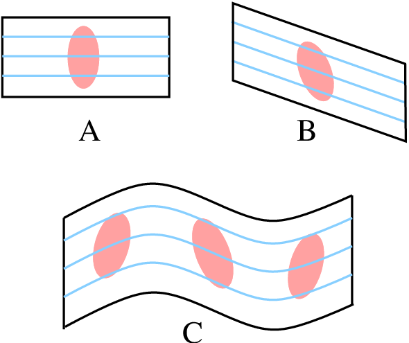
The physical mechanism of anomalous elasticity in nematic elastomers can be visualized by considering the low-energy elastic excitations, illustrated in Fig. 4. A rotation of the nematic director and a simultaneous uniform shear deformation, shown in Fig. 4B, is a soft mode and costs zero elastic free energy com f. It is important to note the total effect of this deformation is not a simultaneous global rotation of the solid and the nematic director. Therefore as shown in Fig. 4C, long wavelength fluctuations of these soft deformations are only penalized by the Frank free energy for distortion of nematic director. As we will show, at finite temperatureXing and Radzihovsky 2003; Stenull and Lubensky 2003a; Stenull and Lubensky 2003b, and/or in the presence of elastomer’s random heterogeneityXing and Radzihovsky 2004, these fluctuations diverge with the system size, and hence necessitate a nonperturbative treatment of relevant elastic nonlinearities. All modes of the elastic deformation that are coupled to the soft modes are strongly affected by these fluctuations, leading to the aforementioned anomalous elasticity. By contrast, because the volume remains fixed in soft deformations, the bulk mode is not coupled to the soft mode. Consequently the bulk modulus of nematic elastomers is only weakly affected by fluctuations.
It is worth stressing that the renormalization group behavior characteristic of nematic elastomers (and other soft solids), where, as displayed in Fig. 3, the low-temperature ordered phase is controlled by a non-Gaussian fixed point, is quite exotic from a field-theoretic point of view. A more standard scenario is an ordered phase controlled by a Gaussian (noninteracting) fixed point, with fluctuations and nonlinearities only qualitatively important when the system is fine-tuned to a critical point, controlling a continuous transition out of the ordered state. In contrast, for nematic elastomers and other soft solids Grinstein and Pelcovits 1981; Radzihovsky and Toner 1999; Bellini et al. 2001; Nelson and Peliti 1987; Aronovitz et al. 1989; Radzihovsky et al. 2001; Ettouham et al. 2005, fluctuations and nonlinearities are important throughout the ordered phase, i.e., no fine-tuning is necessary. Consequently, the whole ordered phase displays the anomalous elasticity with nontrivial and universal power-law correlations, similar to the behavior near a critical point of more conventional systems. It is thus appropriate to refer to a nematic elastomer and other similar soft solids, like the smectic and columnar liquid crystals and flat phase of tensionless polymerized membranes, as a “critical phase” com g.
I.5 Outline
In this paper we give a detailed and pedagogical report of our recent works on the nonlinear elasticity and fluctuations in homogeneous as well as heterogeneous nematic elastomers. Partial results of this study were published earlier in brief communications Xing and Radzihovsky 2003; Xing and Radzihovsky 2004. The remainder of this paper is organized as follows. In Sec. II, we introduce basic concepts for the development of elasticity theory for nematic elastomers and discuss the underlying symmetries as well as the corresponding Goldstone soft modes. Based on these we construct a general elastic free energy for ideal nematic elastomers, in terms of a nonlinear strain tensor which completely encodes the soft modes. We also discuss the relation between this elastic free energy and the neo-classical theory.
In Sec. III, we study the elasticity of nematic elastomers in the context of micropolar elasticity theory. We demonstrate that the conservation of angular momentum ensures that such medium is characterized by a generically asymmetric stress tensor, which encodes angular momentum transfer between the translational and the internal nematic degree of freedom. By enforcing mechanical equilibrium, we derive the stress tensor and the couple-stress tensor of a nematic elastomer as appropriate derivatives of the elastic free energy. We also explicitly calculate the Cauchy stress tensor and the couple-stress tensor for two elastic energy models.
In Sec. IV, we formulate the macroscopic elasticity theory of nematic elastomers at a finite temperature using the constant-strain and the constant-stress thermodynamic ensembles. These two ensembles are related by a Legendre transformation, and contains the same macroscopic physics. We then proceed to construct an effective strain-only description of a nematic elastomer by expanding the elastic free energy in terms of the nonlinear, fully rotationally invariant Lagrangian strain tensor of the nematic state. We derive five Ward identities imposed by the underlying rotational symmetry. These identities relate the coefficients of all anharmonic terms to that of harmonic ones, as well as require a strict vanishing of one of the five elastic harmonic elastic moduli that characterize a uniaxial solid.
In Sec. V, we use this effective theory to analyze the effects of thermal fluctuations on the long-scale elastic properties of ideal, homogeneous nematic elastomers. We first study the fluctuations at the harmonic level and demonstrate that on sufficiently long length-scales, elastic nonlinearities always become qualitatively important for three and lower dimensional elastomers. We then employ the machinery of renormalization group transformation (RG) to systematically study the long-scale effects of thermal fluctuations in the nonlinear theory. Incorporating the most relevant nonlinearities, we compute the resulting long-scale, universal anomalous elasticity of homogeneous nematic elastomers.
In Sections VI and VII, we study the effects of network heterogeneity in nematic elastomers. We first identify the most relevant type of quenched disorder and show that at a harmonic level it leads to distortions relative to the ideal nematic reference state, that diverge for dimensions five and below. To characterize long-scale effects of such distortions we treat the nonlinear elasticity using renormalization group technique and show that the long-scale elasticity of a heterogeneous nematic elastomer is indeed controlled by an aforementioned zero-temperature, finite-disorder fixed point. We calculate the renormalized correlation functions and show that all elastic constants, except the bulk modulus, are singular functions of probing length-scales. Consequently, the stress-strain relation is strictly nonlinear for arbitrary small deformation. We further show that the spatial correlation of the non-affine deformation field acquires anomalous scaling at long length-scales. Finally we conclude this paper with a discussion of experiments and future research directions.
II Symmetries, Soft Modes, and Nemato-Elastic Theory
II.1 Basic ingredients
An ideal nematic elastomer is a homogeneous elastic medium with internal orientational degree of freedom (characterized by the nematic order parameter), which may spontaneously break the underlying, internal rotational symmetry. Similarly to a conventional (fluid) liquid crystal it thus exhibits a high-temperature isotropic phase and a low-temperature nematic phase, which are separated by a thermodynamic phase transition com h. Inside the isotropic phase and for small distortions, its elasticity is described by the conventional elasticity theory of isotropic solids Love 1944; Landau and Lifshitz 1986, characterized by two Lamé coefficients.
A conformation of such -dimensional ordinary elastic medium is described by a -dimensional vector-valued function , which specifies the position of each mass point labeled by , that is also a -dimensional vector. Through out the paper, we will always choose the labeling such that it coincides with the average position of the corresponding mass point in the high-temperature isotropic phase of the system. We shall refer to as the isotropic referential, or Lagrangian, coordinate com i. The coordinate space where the vector “lives” shall be referred to as the isotropic reference space and the corresponding state as the isotropic reference state (IRS). The vector , denoting the spatial position of a mass point in an arbitrary deformed state will be referred to as the current or Eulerian coordinate and the space in which it “lives” as the embedding space. We shall always use symbol , , etc, with a vector on the top for all vectors, and use boldface characters such as and for matrices and rank-two tensors, use symbols , , etc, for unit vectors with magnitude one.
Using a fixed orthonormal coordinate system , we may decompose the vectors as , and . The elastic deformation can be locally characterized by a matrix function
| (1) |
which is usually referred to as the deformation gradient or as the Cauchy deformation tensor. Note that is a “mixed tensor” with one index in the reference space and the other index in the embedding space. They transform differently under rotations in each space.
Starting from the isotropic phase, the isotropic-nematic phase transition is characterized by a development of the nematic order, accompanied by a spontaneous uniaxial strain deformation. The nematic order is characterized by a second rank symmetric traceless tensor field , that naturally vanishes in the isotropic reference state (IRS). In a low-temperature (uniaxial) nematic reference state (NRS), it is given by
| (2) |
where the unit vector is the nematic director that gives the uniaxial nematic direction in the NRS and is the magnitude of that characterizing the strength of nematic order; is the identity matrix tensor. Furthermore, the nematic reference state is related to the isotropic reference state via a spontaneous uniaxial deformation
| (3) |
where and are ratios of a deformation in the directions parallel and perpendicular to the nematic director . Because typical nematic elastomers (and more generally rubber) are characterized by a bulk modulus that is much larger than the shear modulus, the spontaneous deformation is nearly volume preserving, satisfying a constraint , that imposes a relation
| (4) |
The corresponding conformation vector , defined by
| (5) |
specifying average positions of mass points in the NRS is given by
| (6) |
To simplify the notations we shall always use to denote the position of mass point in NRS, i.e.,
| (7) |
and will refer to it as the nematic referential (Lagrangian) coordinates and to the space in which it lives as the nematic reference space.
An arbitrary state of a nematic elastomer is characterized by a pair of fields , which specify the geometric deformation as well as the nematic order, respectively. Note that we can equivalently treat and as functions of the nematic Lagrangian coordinate , in which case we use the notation com j. In the nematic phase, it is often convenient to use the deformation gradient defined relative to the nematic reference state:
| (8) |
Using Eqs. (5,6,7), we readily find the relation between and :
| (9) |
where is the spontaneous deformation, Eq. (3). The relations between the IRS and NRS is summarized schematically by the upper half of Fig. 5.

II.2 Symmetries and nemato-elastic Goldstone modes
Since the rotational symmetry is spontaneously broken in the nematic phase, the Goldstone theorem dictates that in the nematic phase, the ground state must be infinitely degenerate and there must be a soft mode associated with this degeneracy. This soft mode was first predicted by Golubović and Lubensky Golubović and Lubensky 1989 on symmetry grounds. A thorough analysis was then given by Olmsted Olmsted 1994 and in Ref. Lubensky et al. 2002, and so we only give a brief discussion here. As shown in Fig. 5, starting from the IRS (upper left), there is a continuous manifold of different nematic reference states available to the system. One representative is in the upper right, characterized by a director and a spontaneous deformation , Eq. (3). Energetically equivalent nematic reference states can be obtained by first rotating the isotropic reference state by an arbitrary orthogonal matrix (lower left),
| (10) |
and only then have it undergo an I-N transition to a nematic state characterized by a distinct director (lower right), with a nematic order parameter
| (11) |
This transition is accompanied by a spontaneous deformation
| (12) |
It is clear from Fig. 5 that starting from one NRS with a director (upper right), the other nematic ground state (lower right) with a director is accessible via a rotation of a nematic director, combined with a deformation (right arrow in Fig. 5):
| (13) |
We note (as long as is not related to by a rotation ) this is not a simultaneous rigid body rotation of the deformed elastomer and the nematic director in the upper right. Instead, the above combination of a deformation and a director rotation takes the system from one ground state to an elastically distinct but energetically equivalent one, and therefore is the Goldstone soft mode associated with the spontaneously broken rotational symmetry in a solid. Clearly then, in an ideal case the deformation in Eq. (13) costs zero elastic free energy. This soft mode, fully characterized by an arbitrary rotation and the nematic director , is one of the most striking consequence of a spontaneous symmetry breaking, and provides the key to many unusual properties of nematic elastomers. The main purpose of the present paper is to study the local fluctuations of this soft mode and their effects on the long length-scale elastic properties of nematic elastomers.
An arbitrary uniform deformation of the system away from the NRS is described by a triad , where and are the nematic director of the initial and final state respectively, while , defined in Eq. (8), is the deformation gradient defined relative to the NRS. The elastic free energy density with strains measured in the nematic referential coordinates must reflect the symmetries discussed above.
Namely, must be invariant both under an arbitrary global rotation of the nematic reference state and under that of the current state, i.e., it satisfies
| (14) |
where and are two arbitrary orthogonal matrices. More importantly, the elastic energy has to vanish for an arbitrary soft deformation , as given by Eq. (13), i.e.,
| (15) |
with a special case of the director in the final state the same as the initial state given by
| (16) |
More generally, the free energy should be independent of whether deformation is preceded by a soft deformation . Thus the elastic free energy density of a nematic elastomer must satisfy
| (17) |
It clear that Eq. (17) contains Eq. (15) (and hence Eq. (16)) as a special case.
Let us examine the symmetry properties of the neo-classical theory Warner and Terentjev 1996; Warner and Terentjev 2003 for ideal, single domain nematic elastomers. In this theory, the elastic free energy density of a uniform volume preserving deformation is given by
| (18) |
where the tensors and , defined in Eqs. (22), are the so-called step length tensors and are functions of the nematic director in the initial and in the final states, respectively. It is easy to show that indeed the neo-classical theory, Eq. (18) satisfies properties (14-17). However, it also exhibits another symmetry, namely
| (19) |
Physically this corresponds to an invariance of the free energy under a soft deformation applied after an arbitrary deformation. This property does not seem to follow from any underlying symmetry of a nematic elastomer and is therefore not expected to hold in real systems. Thus, this unphysical constraint and associated limitations of the neo-classical theory should be experimentally detectable.
II.3 Invariant strains
It is a generic feature of nonlinear elasticity theories, that there is no unique definition of a strain tensor. For ordinary elastic media, where there is no independent orientational degree of freedom, infinite number of strain tensors can be defined in terms of the deformation gradient com k:
| (20a) | |||||
| (20b) | |||||
where is an arbitrary integer. A common feature of these strain tensors is that they vanish for an arbitrary global rotation. Furthermore, ’s () are tensors (scalars) in the reference space, and scalars (tensors) in the embedding space.
For isotropic solids, e.g., ordinary rubber or glass, either ’s or ’s provide an equally good description of elasticity, with elastic free energy expressible as a function of any of the tensors above. For anisotropic solids, e.g., crystals, tensors provide a natural elastic description, while tensors are inadequate to capture the anisotropy of the reference state.
In the case of nematic elastomers, a priori, none of these strain tensor provide a complete description since they do not contain any information about the nematic director (but see Sec. IV.3). However, as we now show they can be generalized to incorporate the nematic directors of the nematic reference and deformed states. Let us look at the following generalized symmetric strain tensor in the embedding space:
| (21) |
where
| (22a) | |||||
| (22b) | |||||
are the so-called “step length tensors” in the initial and final state respectively. It is easy to see that is a generalization of com l as defined in Eqs. (20): in the isotropic limit, i.e., ,
| (23) |
The generalized strain has many nice symmetry properties. It is invariant with respect to arbitrary rotation in the reference space:
| (24) |
It transforms as a second rank tensor with respect to rotations in the embedding space:
| (25) |
More importantly, it automatically vanishes for arbitrary soft deformations Eq. (13), i.e., satisfies Eq. (15) and Eq. (17), much like the free energy density does:
| (26a) | |||
| (26b) | |||
Because of these symmetry properties, we shall call an invariant strain. A scalar function of the tensor automatically satisfies both Eq. (14) and Eq. (17).

To clarify the origin of the symmetry properties of , we express it in terms of the deformation gradient defined relative to the isotropic reference state. Using Eq. (9) and Eq. (22a) in Eq. (21) we find:
| (27) |
Remembering that is the energetically preferred spontaneous deformation measured relative to the isotropic reference state, if the nematic director of the current state is . Therefore, the tensor inside the square bracket in Eq. (27) describes the nonlinear strain , measured relative to the isotropic reference state, minus its optimal value for given nematic director . It is same as the tensor defined in reference Lubensky et al. 2002, Sec. IV B (Theory with strain and director). In other word, measures the tensorial “distance” between the deformed state and the ground state manifold, as illustrated schematically in Fig. 6. This is the fundamental reason why vanishes for an arbitrary soft deformation.
We note in passing that all other nonlinear strain tensors and , as defined in Eq. (20), can be generalized to the case of nematic elastomers. Both properties Eq. (14) and Eq. (17) are satisfied by the generalization of for arbitrary integer . On the other hand, analogous generalization of does not satisfy the property Eq. (17) and therefore does not provide an adequate description of the elasticity of nematic elastomers.
II.4 Modes of deformation
For convenience of later discussion, we shall let the dimension be an arbitrary integer larger than two. Let be an orthonormal basis of the dimensional embedding space, where is the nematic director in the deformed state com m. This coordinate frame therefore rotates with the nematic director , in strong contrast with the frame that we introduced earlier. It is convenient to introduce two complementary projection tensors in this space:
| (28a) | |||||
| (28b) | |||||
that naturally satisfy the following properties:
| (29a) | |||||
| (29b) | |||||
| (29c) | |||||
| (29d) | |||||
projects out the one dimensional subspace along the nematic director , while projects out the dimensional subspace perpendicular to .
The strain tensor can then be decomposed into different parts using these projectors:
| (30a) | |||||
| (30b) | |||||
| (30c) | |||||
| (30d) | |||||
This decomposition is illustrated in Fig. 7.

Using this basis, as illustrated in Fig. 7, we decompose the strain into an isotropic part and some other traceless parts according to
| (31) |
where is a traceless matrix
| (32) |
a identity matrix, and a scalar and a traceless matrix are given by
| (33a) | |||||
| (33b) | |||||
To illustrate the geometric meaning of the different components of the tensor in Eq. 31, let us consider a special case of small, spatially dependent deformation from the nematic reference state. To lowest order approximation, we need not distinguish the Lagrangian and Eulerian coordinates. We define a phonon field , a linearized symmetric strain tensor , and a linearized antisymmetric strain in a standard way:
| (34a) | |||
| (34b) | |||
| (34c) | |||
| (34d) | |||
where we have adopted the nematic Lagrangian coordinates and have used the shorthand for . We also choose , and consider small fluctuation of the nematic director:
| (35) |

The full expressions for components of in terms of these variables can be obtained by using Eqs. (34) and Eq. (35) in Eq. (21). Up to linear order in and , this leads to:
| (36) |
Consequently describes the isotropic compression/dilation of the solid, i.e., the bulk mode, illustrated in Fig. 8A. We also find that
| (37) | |||||
where we have used the fact that at the lowest order. Therefore describes a dilation (compression) along the axis combined with an isotropic compression (dilation) transverse to this axis (perpendicular subspace), with the total volume conserved, as illustrated in Fig. 8C. We shall call this mode the longitudinal shear mode. The strain component is, up to linear order of the phonon field, given by
| (38) | |||||
where indices and are restricted to the dimensional transverse subspace. Therefore describes shear deformation in the dimensional subspace perpendicular to , as illustrated in Fig. 8D. This mode breaks the uniaxial symmetry and we will refer to it as the transverse shear mode. Up to a linear order, the above three modes, i.e., the bulk, the longitudinal shear, and the transverse shear only depend on the symmetric linearized strain and are the same for nematic elastomers as for ordinary uniaxial solids.
However, the strain operator mixes the symmetric strain with the antisymmetric strain and the director fluctuation . Upto linear order in and , it is given by
| (39) |
where is a dimensionless ratio characterizing the spontaneous anisotropy of the nematic phase. In the limit of a vanishing nematic order, , , and consequently reduces to the linearized symmetric strain, . For a non-vanishing nematic order, however, the strain involves a symmetric strain , a rotation of the solid , as well as a rotation of the nematic director . Strain components qualitatively distinguish a nematic elastomer from an ordinary uniaxial solid. It is clear from Eq. (39) that describes a simple shear in a plane containing and the axis, compensated by an infinitesimal rotation of the nematic director as well as a global rotation of the solid, and vanishes for an infinitesimal soft deformation, where the cancellation between these three contributions is complete. This is illustrated in Fig. 8B.
II.5 Nemato-elastic model
The invariant strain tensor measures deformations relative to the uniaxial ground state manifold of an ideal nematic elastomer, and therefore vanishes for arbitrary soft deformation. Thus, for a uniform deformation, the elastic energy of an ideal nematic elastomer can be expressed as a scalar function of . Indeed, in the neo-classical theory, the elastic free energy per unit volume com n, Eq. (18), can be written as
| (40) |
where we have used the cyclic property of the trace operation and that follows from Eq. (22). Using Eq. (21), the incompressibility constraint can also be written in terms of as
| (41) |
Because of the highly nonlinear incompressibility constraint Eq. (41), the neo-classical theory Eq. (40) is not particularly convenient for our goal of studying long wavelength fluctuations of a nematic elastomer. Furthermore, as we have noted at the end of Sec.II.2, the neo-classical theory exhibits extra unphysical symmetry, Eq. (19), and is thus not the most general theory satisfying physical elastomer symmetries Eqs. (14), (17). We therefore relax the incompressible constraint and expand the elastic free energy in powers of the invariant strain . This removes the aforementioned unphysical symmetry of the neo-classical theory. Linear terms cannot appear since the nematic reference state is a minimum of the elastic free energy. In accordance with the uniaxial symmetry in the nematic phase, five different quadratic terms can appear. Ignoring all higher order terms, the elastic energy density can be expressed as com o
| (42) | |||||
| (43) |
where we have used two different decompositions of , related to each other by Eqs. (33). Note that we have used the coordinate system as illustrated in Fig. 7. The total elastic free energy is then given by integrated over the nematic referential volume element com p
| (44) |
where
is the Jacobian factor relating the Eulerian volume element to the Lagrangian volume element. For most rubbery materials the Jacobian factor is very close to unity (up to ).
The two sets of parameter in Eq. (42) and Eq. (43) are related via:
| (45a) | |||||
| (45b) | |||||
| (45c) | |||||
Inverting the relations (45), we find
| (46a) | |||||
| (46b) | |||||
| (46c) | |||||
Following our discussions of different deformation modes in the preceding subsection, we shall call the elastic constants , and in Eq. (43) the bulk modulus, the longitudinal shear modulus, and the transverse shear modulus, respectively. Generically, rubber is characterized by a bulk modulus that is four to five orders of magnitude larger than all other elastic moduli. Furthermore, as we shall see in Sec. V and Sec. VI, ideal nematic elastomers are actually strictly incompressible due to strong fluctuations that singularly renormalize elastic moduli, driving all (, , and ) but the bulk modulus to zero at long length-scales. This essential difference between the bulk modulus and other moduli (, , ) indicates that Eq. (31) and Eq. (43) provide a more natural parameterization to the invariant strain and the elastic energy, respectively. By contrast, if one insists on using the parameterization in Eq. (42) with independent parameters , , , , one would find, from Eqs. (45) that all renormalized elastic constants except flow to the same limiting value, i.e., to the renormalized non-universal bulk modulus . The essential physics (i.e., strict incompressibility, universal Poisson ratios, etc.) is thus missed in this latter parameterization, hidden in the differences between these renormalized constants and , which go to zero in the long wavelength limit.
We note that by virtue of the invariant strain , the elastic energy (43) vanishes identically for an arbitrary soft deformation, i.e., it satisfies Eqs. (15-(17). On the other hand, since the elastic energy is expanded up to the second order of the strain , it is valid for small value of , i.e., the strained state should be not far away from the ground state manifold. Because of the uniaxial nematic order, the elastic energy (43) of a nematic elastomer bears a resemblance to a conventional uniaxial solid, that to a quadratic order in the nonlinear Lagrange strain tensor (using the decomposition introduced above) is given by Landau and Lifshitz 1986
| (47) | |||||
Although both elastic energies, Eq. (42) and Eq. (47) are characterized by five independent moduli, there is an essential qualitative difference between a conventional uniaxial solid and an ideal nematic elastomer: while the Lagrange strain is a tensor in the reference space and only depends on the geometric deformation , the invariant strain is a tensor in the embedding space and depends both on the geometric deformation and on the nematic director rotation, and more importantly, vanishes for arbitrary soft deformations.
For non-uniform deformations, the elastic energy Eq. (42) and Eq. (43) must be augmented by the free energy cost for distortion of the nematic order, that in 3d is given by the Frank free energy
| (48) | |||||
where , and are the splay, twist, and bending constants, respectively. Again, we have defined the free energy density as the Frank free energy per unit volume measured in the nematic referential coordinate system. Here it is important to note that the gradient operator is defined in the Eulerian coordinates , i.e., , because the nematic director interaction is dominated by the liquid fraction com q.
For small deformation, we can take and make linear approximation of the invariant strain in Eq. (43), in terms of linearized strains , and the director fluctuation . The elastic energy Eq. (43) then reduces to
| (49) | |||||
where
| (50) | |||||
| (51) | |||||
| (52) | |||||
| (53) |
The last term in Eq. (49) is the most interesting one. It explicitly demonstrates our earlier general symmetry assertion that a simple shear can be completely compensated by a combination of the elastomer and the nematic director rotations, and respectively, such that the net elastic energy cost is zero. An infinite set of such soft elastic distortions is specified by a constraint
| (54) |
This complete compensation is a consequence of the spontaneous symmetry broken nematic elastomer state and is the lowest order manifestation of the soft deformation Eq. (13).
If one is primarily interested in the elastic degrees of freedom, then director fluctuations can be integrated out of the Eq. (49), thereby obtaining an effective elastic description purely in terms of the strain . It is easy to show that at the quadratic order this leads to a rotation tensor and that automatically adjust to to satisfy the soft mode constraint Eq. (54). Thus it is quite clear that the resulting effective elastic free energy density has the form Eq. (49), but with the last shear term identically vanishing, a result that was first derived (in a quite a different way) by Golubović and Lubensky Golubović and Lubensky 1989; Lubensky et al. 2002. We thus observe that the elasticity of uniaxial nematic elastomers resembles that of ordinary uniaxial solids, but with key distinction that the transverse shear elastic modulus strictly vanishes, which is guaranteed by the underlying rotational symmetry spontaneously broken in the nematic state.
To illustrate the basic structure of the harmonic theory Eq. (49), let us consider a simple mechanical experiment illustrated in Fig. 9.

With the initial nematic order (uniaxial axis) along , we study the elastic response to a small strain deformation . To avoid the elastic stripe instability Kundler and Finkelmann 1995, we take to be negative, as shown in Fig. 9. To find the equilibrium state we minimize the elastic free energy Eq. (49) with respect to all strain components except . In strong contrast to a stretch along axis, a compression along is stable against an inhomogeneous soft deformation, and therefore and strain components as well as remain zero. We can therefore ignore the term in Eq. (49).
For concreteness we focus on three dimensions, and simplify the analysis by taking the bulk modulus to infinity, a reasonable approximation for elastomers that are essentially incompressible. Minimizing the elastic energy Eq. (49) over , , and for fixed , we obtain:
| (55a) | |||||
| (55b) | |||||
| (55c) | |||||
which satisfy the traceless incompressibility condition
| (56) |
As expected, in this simplest (fluctuation-free) harmonic treatment the compressional elastic response coincides with that of an ordinary uniaxial solid. Because in the incompressible limit the cross-coupling drops out, the ratios between different strain components (i.e., Poisson ratios) only depend on a single ratio . As we shall see later in this paper, long wavelength fluctuations drive this ratio to a universal constant, set by the ratio between the renormalized shear moduli and . The simple experiment illustrated in Fig. 9 allows a direct test of the universal Poisson ratios predicted by our theory.
Although our focus here (and throughout the manuscript) is on the most experimentally relevant uniaxial nematic state, our phenomenological model, Eq. (42) or Eq. (43), can be easily generalized to a biaxial nematic elastomer. Indeed we can define the invariant strain tensor by Eq. (21) for arbitrary -axial nematic order simply by using corresponding -axial step-length tensors and . However, such non-uniaxial nematic elastomer generically has many more elastic constants in its free energy. For example, a three-dimensional biaxial nematic elastomer is characterized by biaxial step length tensors and . All rotational symmetries are broken and the corresponding quadratic elastic free energy density has independent parameters:
| (57) | |||||
where are three mutually orthogonal principle axes of the biaxial nematic order in the deformed state. Similarly a two-dimensional ideal nematic elastomer is characterized by elastic constants and the following elastic free energy density:
| (58) |
where are the principle axes of the nematic order.
We conclude this section by contrasting the differences between the neo-classical elastic model, Eq. (18) and the nemato-elastic model, Eq. (43). While both theories can be formulated in terms of the invariant strain and both capture the full nematic elastomer symmetry, the neo-classical theory has the advantage of simplicity (characterized by only two independent parameters, the shear modulus and the dimensionless ratio ), and can be easily used to describe large deformations. On the down side, as mentioned earlier, the neo-classical model is over-constrained, containing a larger symmetry, Eq. (19) than that exhibited by a generic nematic elastomer. The neo-classical theory is also not well-suited for studying long wavelength fluctuations.
On the other hand, although the Laudau theory Eq. (43) does not have this redundant symmetry, characterized by five elastic moduli, it can only be used for small deformations near the ground state manifold. In the limit of infinite bulk modulus, the moduli and drop out and the Landau theory considerably simplifies to three independent parameters. Furthermore, it allows for a systematic study of long wavelength fluctuations and heterogeneities as well universal properties of nematic elastomers.
III Cosserat, micropolar, and asymmetric elasticity
III.1 Micropolar elastic media
Nematic, as well as other liquid crystalline elastomers, are examples of a wider class of micropolar elastic media Nowacki 1986 that are elastic solids with both translational and rotational degrees of freedom. A proper description of micropolar elasticity therefore falls outside the domain of the classical elasticity theory Landau and Lifshitz 1986. Related to the concept of micropolar elastic media, there is another concept of micropolar fluids, i.e., fluids with broken rotational symmetry. Examples of micropolar fluids include nematic, hexatic, and ferroelectric fluid phases, all characterized by an asymmetric stress tensors. In between micropolar solids and micropolar fluids, there are also systems with orientational order and partial translational order. For example, in a smectic liquid crystal, in addition to the mass-density wave position, whose fluctuations are specified by a phonon field , the orientation of the nematic director field must be specified to fully characterized the state. In the limit of infinitely strong anchoring (which can be shown to be always the case in the long wavelength limit), the director becomes locked to the layer normal, thereby allowing an effective description in terms of purely translational elastic degrees of freedom. Although a three-dimensional material, a smectic liquid crystal is not a three-dimensional solid, since it has rigidity only in one direction alone the layer normal.
Historically com e, the elasticity of micropolar elastic solids was first studied by W. Voigt and the Cosserat brothers back in early 1900’s, and is often referred to as Cosserat media. In the standard micropolar elasticity theory, a deformation of the solid is described by the displacement field as well as an independent rotation vector , with latter specifying the orientation of the “molecules” (which are usually modeled as isotropic rigid bodies) relative to some reference configuration. A distinguishing macroscopic property of such media is that they can transmit torque independent of force. Not being widely noticed for a long time, this subject was revived about half a century later, most notably by Nowacki, Eringen and others Nowacki 1986, in the mechanical engineering and applied mathematics communities, and was renamed as micropolar elastic media. One major motivation underlying these efforts seems to study the elasticity of solids with microstructures. The theories developed by these authors are quite formal and with presentation that parallels the classic work of elasticity by Love Love 1944. They focus on conservation laws, as well as general equations of motion, without paying much attention to the microscopic physical mechanism that leads to the unconventional elasticity. The success of these theoretical efforts on micropolar elasticity is limited by the lacking of well controlled experiments on relevant materials. We note that only quite recently did physicists start to successfully synthesize these elastic solids with internal degree of freedom. Furthermore, most of the research on the micropolar elasticity was concentrated on the isotropic state of the micropolar media, where the coupling between the relative rotation and shear deformation, e.g., the last term in Eq. (49) or Eq. (43), does not appear. As we will show in subsequent sections, this nemato-elastic coupling is in fact the most interesting and most important feature of micropolar elasticity.
For nematic elastomers, the internal orientational degree of freedom is characterized by a unit vector field with two degree of freedom, not a rotation vector with three degree of freedom. In this section, we shall examine the elasticity of nematic elastomers from the view point of micropolar elasticity theory, with the conservation of angular momentum as the central principle. Our discussion shall thereby clarify various aspects of qualitative difference between ordinary solids and nematic elastomers. We will also derive equations that must be satisfied by the stress tensor and the coupled-stress tensor in elastic equilibrium, obtained from the variation of the elastic energy with respect to a virtual deformation and rotation. From these equations (working in 3d) we will find explicit expressions for the true stress tensor and the couple-stress tensor for a uniformly deformed nematic elastomer.
Following the standard convention of the nonlinear elasticity literature, in this section we shall use a slightly different notation than the rest of the paper. We will use to denote the referential (Lagrangian) coordinate and the target space (Eulerian) coordinate com r. A state of an ordinary elastic media is then given by a function where is the time. Let , , be the line, surface, and volume elements of the Lagrangian coordinates. Then the corresponding quantities in the Eulerian coordinates , , are given by standard relations Ogden 1984:
| (59a) | |||||
| (59b) | |||||
| (59c) | |||||
where is the corresponding Jacobian factor.
A local physical quantity , e.g., a certain extensive quantity per unit mass, can be treated as a function of either the Lagrangian or the Eulerian coordinates, i.e.,
| (60) |
We use to denote a material time derivative, i.e., the time derivative of with the Lagrangian coordinate fixed, and use for the time derivative with the Eulerian coordinate fixed. Clearly these two derivatives are related to each other in a standard way
| (61) |
where
| (62) |
is the velocity field.
As the elastic medium deforms, the region that it occupies in the Eulerian coordinate space changes with time. The corresponding region in the Lagrangian coordinate space remains constant in time. Taking the mass density , measured in the Lagrangian coordinates to be spatially uniform, we have:
| (63) |
since the material time derivative commuting with integral over the Lagrangian coordinates. The mass density, , measured using the Eulerian coordinates is related to by
| (64) |
We can use this to express Eq. (63) in terms of the Eulerian coordinates:
| (65) |
Eqs. (65) and (63) are referred to as the transport theorem Ogden 1984 in elasticity literature.
III.2 Conservation of angular momentum in conventional elastic media
Let (Eulerian coordinate) be an arbitrary point inside an elastic media and a surface element passing through , where is the unit normal vector. The stress vector field is defined as the elastic force that is exerted on one side of the surface element from the other side. The famous Cauchy’s theorem Love 1944; Ogden 1984 then dictates that the stress vector depends linearly on the vector and there exists a stress tensor field , referred to as the Cauchy stress, or the true stress, given by
| (66) |
As we will see, for ordinary liquids or solids, conservation of angular momentum requires the Cauchy stress tensor to be symmetric, i.e., . We can also express the stress vector in terms of the Lagrangian surface element :
| (67) |
through the so-called nominal stress tensor Ogden 1984, related by Eq. (59b) to via:
| (68) |
The nominal stress is generally not symmetric.
For a deformed body, Newton’s second law dictates that the rate of change of total linear momentum is given by the total force acting on the body:
| (69) |
which consists of the bulk and surface contributions, with the body force per unit of mass acting at a point . Applying the transport theorem on the left hand side, as well as the Gauss theorem on the right hand side, we find the following equation of motion for an (ordinary or micropolar) elastic solid:
| (70) |
where is a vector with components . Since this must be true for an arbitrary volume element, Eq. (70) must be satisfied by equality of integrands and thus leads to a local field equation of motion
| (71) |
referred to as Cauchy’s first law of motion. For an elastic body in equilibrium and under a vanishing body force, we recover the well known result that static stress field is divergenceless in the absence of external forces, i.e., .
The angular momentum of an ordinary solid is due to the center of mass motion of its constituents (atoms, molecules, colloids) and is given by
| (72) |
where volume is not to be confused with velocity . The time derivative of the angular momentum is given by the total torque acting on the elastic body:
| (73) | |||||
where we used the transport theorem, Eq. (65) and Cauchy’s first law of motion, Eq. (71). Defining a pseudo-vector associated with the antisymmetric part of by:
| (74) |
it is easy to see that
| (75) |
Using this identity together with Gauss’s theorem in Eq. (73) we find
| (76) |
For a vanishing body force , the bulk contribution to angular momentum must be locally conserved, with only an external surface stress contributing to a change in . From above expression this is clearly true if and only if . We therefore find Cauchy’s second law of elasticity, namely, that in an ordinary solid the Cauchy stress tensor must be symmetric.
III.3 Conservation of angular momentum in nematic elastomers
A nematic elastomer is an anisotropic micropolar elastic medium, and its complete description is characterized by the mapping and the nematic director field . The time dependent variation of the nematic director gives an additional intrinsic contribution, to the total angular momentum,
| (77) |
The extrinsic part , defined in Eq. (72), gives a contribution associated with the motion of the center of mass of the molecules. The interaction between the translational and orientational degrees of freedom allows an exchange between the intrinsic and extrinsic angular momenta, and thus, neither is separately conserved com s. The total angular momentum, is of course always conserved. Going back to Eq. (76), we see that for nematic elastomers, the antisymmetric part of the Cauchy stress tensor, is generally nonzero, describing the production of the extrinsic angular momentum due to the coupling between translational and orientational degrees of freedom.
To study the intrinsic angular momentum, we need to introduce two physical quantities special to micropolar media. Adopting the terminology from the elasticity literature Nowacki 1986, the body torque, , is the external torque (e.g., due to an external magnetic field) per unit of volume acting on the nematic degrees of freedom. The couple-stress vector is defined as the torque transmitted through an infinitesimal surface element , solely due to the distortion of nematic director across the surface. Clearly this torque acts on the orientational degrees of freedom, i.e., the nematic director com t. One can extend the Cauchy’s theorem and show that the couple-stress vector also depends linearly on and therefore can be written as the contraction between and the couple-stress tensor :
| (78) |
The couple-stress tensor describes the torque transmitted through a unit surface area due to a distortion of the nematic order, instead of a geometric deformation com u.
From a general principle, the rate of change of the total angular momentum is given by the total torque, which is given by combination of the body force and body torque acting on the bulk, and by the stress and couple-stress vectors acting on the boundary:
Subtracting Eq. (76) from Eq. (), we find the rate of change of the intrinsic angular momentum
| (80) |
In the absence of body force and torque as well as the boundary stress and couple-stress, Eqs. (76) and (80) reduce to
| (81) |
demonstrating that the antisymmetric part of the Cauchy stress tensor describes angular momentum transfer between translational and rotational degrees of freedom of a micropolar elastic medium.
III.4 Equilibrium conditions, stress and couple-stress
The total free energy of an ideal nematic elastomer consists of the elastic energy as a function of and , as well as the Frank energy Eq. (48). External body forces, such as those due to e.g., a gravitational or magnetic fields, can also be easily included. For example the free energy associated with the interaction a magnetic field and the nematic director field is given by
| (82) |
that induces body torque. We note that the energy density is defined with respect to unit volume in Lagrangian coordinate and the integration is over the Eulerian coordinates .
To derive the equilibrium conditions, let us apply external force and torque on the surface element at the boundary. We consider an infinitesimal variation of the equilibrium state, i.e., translation of the center-of-mass Eulerian coordinate as well as rotation of the nematic director field as follows,
| (83a) | |||||
| (83b) | |||||
| (83c) | |||||
Operationally, we first rotate the nematic director by without deformation, and then translate each point (together with the rotated director ) to without rotation of the director field. The external traction com v on the boundary introduces two following terms in the total free energy:
| (84) |
The force couples to the translational degree of freedom while the torque couples to the rotational degree of freedom . The total free energy of nematic elastomer under external boundary traction is then given by
| (85) |
where for convenience, we included a Lagrange multiplier term to ensure that the constraint that is a unit vector field is satisfied.
In equilibrium, the first-order variation of the total free energy must vanish. Since the referential volume element in Eq. (85) is invariant under the variation of the current coordinates , the variation of the total elastic energy is given by
| (86) | |||||
Let us look at the variation of the different part of the bulk free energy separately. The elastic free energy density is a function of the deformation gradient and the nematic director . (It is also a function of the initial director , which does not change in the variation.) Under the variation Eqs. (83) the deformation gradient changes as follows:
| (87) | |||||
| (88) |
where to avoid confusion, we use Roman indices , , , etc., to label Eulerian coordinates and use Greek subscripts , , etc., to label Lagrangian coordinates. The first-order variation of the elastic free energy is therefore given by
| (89) | |||||
The Frank free energy density is a function of both the director and its gradient . Under the variation (83), the gradient changes as follows:
| (90) |
which, using Eqs. (83), to the lowest order gives
| (91) |
The first-order variation of the Frank free energy is therefore
| (92) | |||||
where
| (93) |
Finally, the magnetic free energy density , as given by Eq. (82), is a function of the nematic director only. The variation of is therefore given by
| (94) | |||||
Substituting Eq. (89), Eq. (92), Eq. (94) and Eq. (84) into Eq. (86), and performing integration by parts appropriately, we arrive at
| (95) | |||||
At mechanical equilibrium, each volume and surface integral in the left hand side must vanish separately.
Let us first look at the surface integral Eq. (), which is linear in . Since by definition is the th components of the external force per unit area acting on the surface element with normal , it has to be balanced by the corresponding component of elastic force, i.e., the Cauchy stress tensor. We immediately see that the remaining terms in the surface integrand must be the Cauchy stress tensor , giving us an important constitutive relation for the stress tensor field:
| (96) |
For the convenience of later discussion, we separate the stress tensor into two parts,
| (97) |
where due to the elastic deformation, and due to a distortion of the nematic director field are given by
| (98a) | |||||
| (98b) | |||||
For a conventional solid, there is no Frank free energy , and therefore the stress tensor is solely given by in Eq. (98a). Furthermore, rotational symmetry in the embedding space implies that the elastic energy must be a function of the metric tensor defined as
| (99) |
which then gives for the Cauchy stress tensor of an ordinary solid
| (100) |
which (as expected on general grounds discussed above) is obviously symmetric.
Let us now calculate the stress tensor for an ideal nematic elastomer. For the neo-classical elastic energy, Eq. (40), to impose the incompressibility constraint, we introduce a Lagrange multiplier , physically corresponding to the pressure. We then find that the elastic stress tensor is given by
| (101) |
which is clearly asymmetric, unless commutes with . The pressure term is always isotropic and symmetric regardless of the deformation, as one would expect.
A different form of the stress tensor is obtained for our phenomenological elastic model, Eq. (43). A standard but somewhat tedious calculation gives
| (102) |
which is also generically asymmetric.
Let us next turn to in Eq. (98b), derived from the Frank free energy. It is non-vanishing only for an inhomogeneous configuration of the director field. Except for the isotropic pressure term, which can be associated instead with , is identical to the Ericksen stress tensor de Gennes and Prost 1993 studied extensively in nematic liquid crystals literature. Using Frank free energy, Eq. (48) inside Eq. (98b) we find
| (103) | |||||
that is also generically asymmetric, unless all Frank elastic constants are the same.
Let us now look at the bulk term (volume integral) in Eq. (95) associated with the variation . It is clear that the integrand describes the total force per unit volume acting on the element . Indeed the integrand is identical to , with the Cauchy stress tensor given by Eq. (96). Mechanical equilibrium then implies
| (104) |
corresponding to a force balance equation of ordinary solids, in the case of a vanishing body force.
Similarly, the integrand in the surface integral of Eq. (95) involving orientational degrees of freedom must also vanish. Since the tensor is the th component of the external torque per unit area acting on the the surface element with normal , it must be balanced by the corresponding component of the couple-stress term, defined in Eq. (78). Using Eq. (83c) to relate to , we see that the couple-stress tensor must be given by
| (105) |
Substituting the Frank free energy Eq. (48) into Eq. (105) we find
| (106) | |||||
Similar to the stress tensor , the couple-stress tensor is nonzero only if the nematic director field is non-uniform.
Finally, we look at the integrand of the bulk term in Eq. (95) linear in . Defining a local molecular field acting on the nematic director by
| (107) |
bulk torque balance requires a vanishing of this integrand. This then gives a torque balance equation
| (108) |
which imposes an equilibrium orientational constraint that the local molecular field must be parallel to the nematic director. We do not analyze the molecular field in detail in this work.
IV Nonlinear elastic model of homogeneous nematic elastomers
IV.1 Stress versus strain ensembles
The main objective of this paper is to study the effects of long wavelength fluctuations on the macroscopic elasticity, e.g., the stress-strain relation, of an ideal nematic elastomer. To formulate the problem, we need to consider the relation between fluctuations and finite temperature elasticity in some detail. At finite temperature, mass points in an elastic media fluctuate around their equilibrium positions, regardless of whether or not the system is coupled to an external traction. On the other hand, an external traction causes a macroscopic deformation, which changes equilibrium positions of mass points. Furthermore, the spectrum of the fluctuations may also be modified by a macroscopic deformation.
The central quantity we want to calculate is the elastic free energy, as usual obtained as a sum over all elastic configurations with an appropriate Gibbs-Boltzmann weight, determined by the elastic energy discussed in the previous section. It then determines a macroscopic elasticity, renormalized by long wavelength fluctuations. The free energy can be computed either as a function of the imposed macroscopic strain tensor and the nematic director, or as a function of the external traction. The choice of the macroscopic control variable (strain or traction) amounts to a choice of a statistical ensembles within which to study thermal fluctuations. As usual, we expect that in the thermodynamic limit, macroscopic quantities are independent of the choice of the ensemble.
Let us first look at the constant strain ensemble by fixing the macroscopic deformation gradient and the nematic director . For simplicity, we shall only study the case where and are uniform. We shall switch back to the notations we introduced in Sec. II, using for the nematic referential coordinates and for the deformed (target) coordinates. To compute the thermodynamics (e.g., the partition function) we need to sum over all fluctuations of the position field and the nematic director field around their equilibrium values. Naturally, we parameterize these two fields in terms of the phonon displacement field, and the nematic director fluctuation, , defined by
| (109) | |||||
| (110) |
Expressing the Landau elastic energy, Eq. (43) in terms of these fields, we obtain the elastic “Hamiltonian” functional . Since and are local fluctuations, they have well-defined Fourier transformations com w. The corresponding thermodynamic potential, given by
is the elastic free energy, as a function of the macroscopic deformation and the average nematic director . In above functional integrals a short distance (large momentum) cutoff is implicit, set by the lattice constant in crystalline materials and polymer network mesh size in elastomer materials and we are using units in which the Boltzmann constant is .
To calculate the functional integral in Eq. (), we first expand the elastic Hamiltonian around its minimum for the given and , which, baring the possibility of an elastic instability, is given by and , i.e., a uniformly deformed reference state. The zero-th order (tree level) approximation to the functional integral is then simply given by the saddle point approximation, i.e., by setting and in the integrand of Eq. (), i.e.,
| (112) |
This is just the Landau theory, that does not take into account any long wavelength fluctuations.
To systematically address the effects of fluctuations on the macroscopic elasticity beyond the Landau (mean-field) approximation, we expand the elastic energy in terms of the phonon field and the director fluctuation , and calculate the functional integral Eq. () order by order in corresponding nonlinearities. These fluctuations are generically important for all soft solids. As we discussed in Sec. I, for the particular case of ideal nematic elastomers, the fluctuations of nemato-elastic Goldstone modes lead to qualitative breakdown of perturbation theory in the thermodynamic limit, as well as necessity of a renormalization group analysis.
We can also study the constant traction ensemble, by introducing a boundary traction term, expressed in terms of the Lagrangian coordinates and the external traction tensor using Eq. (59b):
| (113) |
For simplicity we shall focus on the case of a vanishing external torque traction, .
In the case where the external traction tensor is independent of , we can use Gauss’s theorem to rewrite com x as
| (114) |
a form that confirms that the deformation gradient and the traction tensor are conjugate variables. Therefore, in equilibrium, is equal to the nominal stress tensor, as introduced in Eq. (68). In fact this explains the notation we used in Eq. (113).
The thermodynamic potential for this ensemble can then be calculated by summing over all elastic configurations with the modified Gibbs-Boltzmann weight:
| (115) |
As usual the thermodynamic potential , Eq. (115) and the elastic free energy Eq. () are related by a Legendre transformation com y:
| (116) |
where is the system volume and is the solution to the following equation
| (117) |
This is precisely the relation between the macroscopic nominal stress tensor and the macroscopic deformation gradient Ogden 1984, both of which can be directly measured in experiments.
IV.2 Referential coordinates at finite temperature
As defined in Sec. II, the nematic reference state minimizes the elastic Hamiltonian and thus precludes the appearance of terms linear in the invariant strain tensor . However, in the presence of thermal fluctuations and elastic nonlinearities, the average position of a mass point is not the same as its nematic referential coordinate . Since the nematic referential coordinate and the average position differ only at finite temperature, their difference (to lowest order) must be proportional to , and inversely proportional to an elastic modulus.
For an isotropic solid, symmetry dictates that and can only differ by a scalar factor and therefore the associated modulus must be the bulk modulus, :
| (118) |
where is the microscopic cutoff length-scale. For ordinary isotropic rubber we have and therefore the difference between the referential coordinate and the average position of a mass point is negligible. In contrast, for an anisotropic elastomers such as a nematic elastomer, the relation between and involves other, significantly smaller elastic constants, which are comparable with . Therefore, generically thermally induced deformation of the average position is non-negligible, particularly near the I-N transition. For a given elastic Hamiltonian, this relation can be systematically computed and in principle is experimentally accessible.
Because of this non-negligible difference between and there are two (in principle equivalent) complementary descriptions of the elastic theory of a nematic elastomer. One, most conceptually clear formulation is in terms of phonon modes expanded about a coordinate system defined by . The advantage of such approach is that the computed renormalized elastic free energy is by construction minimized by a vanishing phonon displacement, i.e., precludes any linear terms in the nonlinear strain tensor . A technical disadvantage is that the elastic Hamiltonian (that does not include long wavelength fluctuations) will then necessarily admit terms linear in , whose coefficients are adjusted order by order in perturbation theory so as to ensure that the renormalized elastic free energy is free of such linear terms com z. The latter is thus quite cumbersome to work with. An alternative, technically more convenient approach is to choose the nematic reference coordinate system , which ensures that instead the elastic Hamiltonian is free of terms linear in the strain. The unavoidable price of this is that such linear terms will then be generated in the renormalized elastic free energy, as a signal of a shift in the elastic minimum configuration. These terms will be discussed in much more detail when we carry out the renormalization group analysis in later sections com.
Thus, for convenience we will always choose the nematic referential coordinates to label mass points and about which to expand phonon fluctuations. Nevertheless, our final results in this work will of course be independent of the choice of the reference state.de Gennes and Prost 1993
IV.3 Strain-only nonlinear elastic model
We are interested in the long wavelength elastic fluctuations in nematic elastomers, i.e., fluctuations of the phonon and the nematic director fields around their equilibrium values. In thermal equilibrium, the Gibbs-Boltzmann distribution of these fluctuations is controlled by the coarse-grained elastic Hamiltonian functional, Eq. (43), augmented by the Frank energy Eq. (48) for the distortion of nematic order. Being fully invariant under rotations as well as arbitrary soft deformations, this energy functional is rather complicated, containing a large number of nonlinearities, most of which are irrelevant at long length-scales. To analyze effects of fluctuations, we therefore look for a simpler, minimal model formulation, which from the start contains only those nonlinearities that survive at long length-scales. Furthermore, focusing on the elastic degrees of freedom, we will integrate out the nematic director fluctuation in the partition function and obtain an effective theory in terms of only the translational degree of freedom . This operation is well justified if the nematic director is tightly coupled to the elastic media, such that the fluctuaftions of the nematic director from its energetically favored direction (determined by the elastic degrees of freedom) are small. This condition is always satisfied com — and is quite similar to the locking (at long length-scales) of the nematic director fluctuations to the local layer normal fluctuations in a smectic liquid crystal, thereby allowing a well-known purely elastic description of smectic liquid crystals.
A “strain-only” elastic model can be obtained by integrating out the nematic director fluctuations from the Hamiltonian (43), formulated in the nematic state. However, to clarify the role of the spontaneous symmetry breaking and to simplify the analysis it is more convenient to do this in a model formulated in the isotropic phase, i.e., expressed in terms of conformational degrees of freedom relative to the isotropic reference state and the nematic order parameter . Integrating out the nematic order parameter, leads to an effective elastic energy functional in which the effective shear modulus changes sign at the I-N transition Golubović and Lubensky 1989; Lubensky et al. 2002, thereby inducing a uniaxial distortion of the elastomer matrix. Expansion about the resulting nematic reference state then gives the sought-after purely elastic description of the nematic elastomer.
Our goal is to deduce the most general form of the resulting elastic Hamiltonian, carefully ensuring its underlying rotational and translational invariance. To ensure these conditions we take it to be the most general scalar function of the metric tensor , defined in Eq. (99). Without loss of generality, we can express it as a function of the following scalar quantities
| (119) |
which are rotationally invariant both in the reference space and in the embedding space. In three dimensions, the metric tensor has only three eigenvalues, ensuring that first three invariants are independent com.
Hence the elastic Hamiltonian is a function of , , and :
| (120) |
In the high-temperature isotropic phase, the elastic Hamiltonian is minimized by , for which , obviously corresponding to the isotropic reference state. In the low-temperature broken-symmetry phase, the elastic energy is minimized by the nematic reference state (NRS), characterized by a uniaxial metric tensor
| (121) |
where , given by Eq. (3), is the spontaneous deformation accompanying the I-N transition. Inside the nematic phase, we can expand the elastic energy Eq. (120) around the NRS:
| (122) | |||||
where
| (123a) | |||||
| (123b) | |||||
| (123c) | |||||
and we have truncated the series at the second order in . Since, by definition ’s are fully rotationally invariant, the rotational symmetry as well as the associated soft mode of the nematic phase are guaranteed by every term in Eq. (122) and are not compromised by the truncation.
To make contact with elasticity theory we express the scalars in terms of the more familiar nonlinear Lagrange strain tensor defined relative to the nematic reference state:
| (124) | |||||
| (125) | |||||
where in the last expression we used Eq. (34a) to express in terms of the phonon field . To this end we make use of the relation Eq. (9) between deformation tensors in the isotropic and nematic reference states, finding:
| (126a) | |||||
| (126b) | |||||
where we defined
| (127) |
Choosing the nematic director of the NRS to be along the axis, we may express the tensor as a matrix:
| (128) |
Substituting Eqs. (126) into Eq. (122) and rearranging the series in the order of increasing powers of the Lagrange strain tensor , we obtain an effective elastic free energy for nematic elastomers with spontaneously broken rotational symmetry:
| (129) | |||||
where repeated subscripts , , are summed over transverse components, only. In above, we have only kept the most important terms, i.e., those that are relevant in the renormalization group sense, as we will verify a posteriori. The values of the eleven coefficients appearing in Eq. (129) are listed in Appendix A.
Not all of the eleven coefficients in Eq. (129) are independent to each other. It is straightforward, although tedious, to check that these coefficients, as given by Eqs. (303), satisfy the following five Ward identities:
| (130a) | |||||
| (130b) | |||||
| (130c) | |||||
| (130d) | |||||
| (130e) | |||||
where
| (131) |
are two dimensionless ratios characterizing the anisotropy of the nematic phase. Therefore out of eleven there are only six independent parameters in Eq. (129). The five Ward identities, Eqs. (130) reflect the underlying rotational symmetry in the isotropic reference state, spontaneously broken by the nematic state.
We note that although we have derived these identities in three dimensions, as we explicitly show in Appendix B, they actually hold in arbitrary dimensions , generalized by simply allowing indices to range over all transverse directions. The elastic Hamiltonian, Eq. (129) and the set of Ward identities Eqs. (130) agree with Eq. (4.3) and Eqs. (4.4) of Ref. Stenull and Lubensky 2003b, after appropriate redefinition of various constants. The correspondence is established in Table 1.
| This work | |||||||||||
|---|---|---|---|---|---|---|---|---|---|---|---|
| Reference Stenull and Lubensky 2003b |
As we have already discussed in Sec. IV.2, it is convenient to choose and in Eq. (128) such that the nematic reference state minimizes the elastic Hamiltonian Eq. (129). This ensures that the coefficients and of linear terms are exactly zero, which further reduces the number of independent parameters in Eq. (129) to four. More importantly, this choice, when combined with the first Ward identity Eq. (130a), dictates that the shear modulus strictly vanishes in the nematic phase, as we have shown in a complementary way in Sec. II. As emphasized there, a vanishing of without any fine-tuning is a consequence of the underlying rotational invariance of the isotropic reference state and is the lowest order manifestation of the corresponding soft Goldstone mode. This feature qualitatively distinguishes a nematic elastomer from an ordinary uniaxial solid, whose corresponding modulus in Eq. (47) is generically nonzero.
The other four Ward identities, Eqs. (130b-130e), dictate that the coefficients of all anharmonic terms in Eq. (129), , , and , are completely determined by the remaining quadratic coefficients, the elastic moduli . As we will see in the next section and as is clear from general symmetry principles from which these arise, these relations are preserved in the presence of fluctuations. Using these relations, we can define an “effective” nonlinear strain tensor with components:
| (132a) | |||||
| (132b) | |||||
where is defined in Eq. (131), and indices and are limited to the perpendicular subspace . The elastic Hamiltonian Eq. (129) then reduces to
| (133) |
which, after supplemented with the curvature energy corresponding to the Frank free energy of the nematic director, will be the form we will use for further study of thermal fluctuations and network heterogeneities.
IV.3.1 Two-dimensional nematic elastomer
The same analysis can be carried out straightforwardly for a two-dimensional nematic elastomer. An important property special to the two-dimensional case, is that the subspace perpendicular to the nematic order is one-dimensional, and thus has no shear mode (characterized in higher dimensions by the modulus ) associated with the transverse subspace.
Consequently, the effective elastic Hamiltonian for a 2d nematic elastomer is given by:
| (134) |
where we chose the nematic director to be along the -axis. The nonlinear strain components and are
| (135a) | |||||
| (135b) | |||||
where . We will leave the analysis of this very interesting two-dimensional model for a future investigation.
IV.4 Relevant nonlinearities and the minimal strain-only elastic model
As we shall see later in this work, the nonlinear elastic model, Eq. (133) is an interesting coupled combination of a smectic-like and columnar-like nonlinear elasticities, involving and , respectively. Experience with the nonlinearities in the presence of fluctuations in these two systems Grinstein and Pelcovits 1981; Grinstein and Pelcovits 1982; Ettouham et al. 2005 suggests that it is the former that are more relevant. We will verify this rigorously a posteriori in Sec. V.1. Thus, anticipating a stronger relevance of elastic nonlinearities to long length-scale fluctuations, we substitute Eq. (125) into Eq. (132) and Eq. (133), and only keep those anharmonic terms (smectic-like nonlinearities) that are proportional to , ignoring all others. It is straightforward to show that this amounts to making the following replacements in Eq. (133):
| (136a) | |||||
| (136b) | |||||
where is defined in Eq. (131).
In order to streamline the notations, we further rescale the phonon fields by
| (137a) | |||||
| (137b) | |||||
and absorb an overall factor of the elastic Hamiltonian by redefining all the elastic constants:
| (138) |
In order to stabilize soft-mode phonon fluctuations, the Hamiltonian in Eq. (133) must be augmented by the the Frank free energy, Eq. (48), using the relation Eq. (54) to eliminate director fluctuations in favor of the phonon fields. Furthermore, since we are most interested in the fluctuations of the phonon field, which in the momentum space is controlled by the pole , it can be easily shown that both the bend () and twist () term are (dangerously) irrelevant in the RG sense com. We will therefore ignore these two terms for the purpose of the RG analysis, and to simplify the notation will use to denote the splay modulus.
The resulting minimal elastic Hamiltonian density has the following form:
| (139a) | |||||
| (139b) | |||||
where the components of the (rescaled) effective strain tensor now become
| (140a) | |||||
| (140b) | |||||
and
| (141a) | |||||
| (141b) | |||||
| (141c) | |||||
The elastic constants (bulk modulus), (longitudinal shear modulus), (transverse shear modulus) and have already been defined in Eqs. (45).
The elastic nonlinearities contained in different modes of deformation are particularly interesting. Qualitatively speaking, the relevant elastic nonlinearities arise from the coupling between various modes of deformation with the soft mode. It is the fluctuations of the soft mode that renormalize various elastic constants and lead to anomalous elasticity. We observe that the bulk mode
| (142) |
| Moduli | ||||
|---|---|---|---|---|
| Descriptions | Bulk Mode | Longitudinal Shear | Transverse shear | Soft Mode |
| N/A | ||||
| Eq. (39) |
does not contain any relevant nonlinearities. This is due to the fact that the soft deformation Eq. (13) preserves the volume and therefore its local fluctuations do not couple to the bulk mode. Consequently we expect that renormalization of the bulk modulus is qualitatively unimportant. On the other hand, from Eqs. (141) and Eqs. (140) we observe that longitudinal shear mode
| (143) |
and the transverse shear mode
| (144) | |||||
do involve relevant elastic nonlinearities. We therefore expect that the renormalization the longitudinal and transverse shear moduli by fluctuations to be qualitatively important. These expectations will be verified by explicit RG calculations in the next section.
We emphasize the structural similarity between Eq. (139b), Eq. (43), and Eq. (49), with the only exception that the term with the coefficient in Eq. (43) and Eq. (49) is replaced by the term with the coefficient in Eq. (139b). Indeed the elastic free energy Eq. (139b) can be obtained from Eq. (43), augmented by the Frank free energy Eq. (48), by integrating out the fluctuations of nematic director, and dropping irrelevant nonlinearities. This procedure replaces the term by the curvature term.
Finally we note that we have represented the bulk, longitudinal shear, and transverse shear modes in terms of the invariant strain , the linearized strain tensors and (Sec. II), as well as the effective strain tensor (the current section). At the linear order in the phonon field, they all agree with each other. In contrast, because the soft mode involves both strain deformation and rotations of nematic director, it cannot be expressed in terms of alone since the latter does not contain . Thus, the soft mode only appears indirectly in the current description, through an exact vanishing of and the form of the nonlinear strain tensor . The relations are summarized by Table. 2.
The effective strain-only model, Eq. (139) will be the starting point for all of our further analysis of thermal fluctuations in the presence of elastic nonlinearities.
V Long-scale thermal elasticity of a homogeneous nematic elastomer
In this section we use the effective elastic model derived in the previous section, Eq. (139) to study the long-scale properties of a nematic elastomer in the presence of thermal fluctuations.
V.1 Harmonic phonon fluctuations
We begin by studying thermal fluctuations within a harmonic approximation, ignoring all elastic nonlinearities in the model, (139b). As mentioned above, this is equivalent to going back to the harmonic theory, Eq. (49), supplemented by Frank free energy, and integrating out the director fluctuation . To the lowest order at long wavelength this amounts to the nemato-elastic coupling in Eq. (49) simply enforcing the replacement
| (145) |
in the Frank free energy Eq. (48). The resulting quadratic effective elastic energy is then given by
| (146) | |||||
where we have absorbed some constant factors into the Frank elastic constants (splay) and (bending). The twist term () turns out to be less relevant than and , and therefore is ignored in Eq. (146). Except for the last two terms (from Frank free energy), Eq. (146) is identical to the quadratic (in phonon field ) parts of the nonlinear elastic Hamiltonian Eq. (133).
In terms of the Fourier transform of the phonon field
| (147) |
the harmonic elastic Hamiltonian takes the form
| (148) |
where indices and are summed over all dimensions, and the kernel matrix is given by
| (149a) | |||||
| (149b) | |||||
| (149c) | |||||
The harmonic phonon correlation functions
| (150) |
can be calculated using the equipartition theorem or equivalently by performing above simple Gaussian integral. They are given by
| (151) |
where as usual is related to via:
| (152) |
The components of the propagator matrix are fairly complicated. For example, is given by
| (153) |
where is a wavevector-dependent constant
| (154) |
Since we are most interested in small (long length-scale) properties, the dependent term in the denominator of Eq. (154) is generically much smaller than the independent term , and therefore can be ignored com. Therefore we may approximate as
| (155) |
where
| (156) |
The correlator Eq. (155) is identical to the harmonic phonon correlation function of a conventional smectic liquid crystal de Gennes and Prost 1993 with and the modulus for layer compression and layer bending, respectively. In three dimensions, the real space mean-squared fluctuations of the phonon field are given by:
| (157) | |||||
where is the system size and the small cutoff length-scale, set by the molecular size. The fact that diverges with the system size suggests a breakdown of the harmonic elasticity theory and the qualitative importance of elastic nonlinearities that have so far been ignored. As in the case of smectic liquid crystal, we expect that the elasticity of three- (and two-) dimensional nematic elastomers is dominated by long wavelength fluctuations of the phonon field.
We can use Eqs. (45) to express as function of , , and . In the limit of an infinite bulk modulus, i.e., with , and fixed, we find approaching a finite limit
| (158) |
Therefore in this limit, the correlation function of field simplify considerably, becoming independent of the bulk modulus . We will see that the same result holds for other correlation functions as well. Physically, for a large , the bulk mode is essentially frozen out, and as a result does not play any role in long wavelength fluctuations.
Matrix inversion of also gives the harmonic correlations of :
| (159) |
where
| (160a) | |||||
| (160b) | |||||
| (160c) | |||||
and
| (161) |
are the longitudinal and transverse projection operators (with respect to ) in the dimensional subspace perpendicular to . Eq. (159) is similar in structure to the harmonic phonon correlations of a columnar liquid crystal Radzihovsky et al. 2001; Ettouham et al. 2005. A straightforward calculation shows that real space fluctuation of remains finite in three dimensions. Therefore the long wavelength fluctuations of the phonon fields, are qualitatively unimportant as compared with those of . This qualitative difference between the phonon fields and is a result of spontaneous broken rotational symmetry in an originally isotropic system. By contrast, in ordinary uniaxial solids, all phonon fluctuations remain finite in three dimensions, thus leading only to quantitative corrections to properties of conventional solids.
The cross correlation functions between and are given by
| (162) | |||||
| (163) |
where
| (164) |
and is the volume of the system. For a sufficiently small , can be approximated by
| (165) | |||
where
| (166) |
V.2 Naive scaling and critical dimension
To study fluctuations in the nonlinear elastic theory beyond the harmonic approximation of the previous subsection, one might naively hope to perform a perturbative expansion in the nonlinear elastic terms. However, a standard analysis, which is relegated to Appendix C shows that such direct perturbation theory is hopelessly divergent at long length scales, as already suggested by divergent phonon fluctuations in e.g., Eq. (157).
Thus, similarly to systems near a critical point (but here applied throughout the nematic phase), to treat elastic nonlinearities we need to employ the machinery of the renormalization group transformation (RG) Wilson 1983; Fisher 1974; Ma 1973 which establishes relations between physical quantities (e.g., correlation functions) at different length-scales. These relations then allow us to extract universal long-scale nonperturbative (in nonlinearities) properties of the system from their perturbatively computable short-scale versions.
To this end, we need to study the property of the system under rescaling of length-scales and coarse-graining (thinning) of degrees of freedom. This procedure, executed explicitly in Appendix C, is quite nontrivial in the presence of nonlinearities. However, it simplifies considerably to zeroth order in nonlinear terms, becoming equivalent to a rescaling transformation on the “bare” Hamiltonian.
Applying this to the nematic elastomer model, Eq. (139b) it is not difficult to see that it is invariant under each of the following two rescaling operations, with an arbitrary rescaling factor:
- 1.
Rescaling of axis:
(167a) (167b) (167c) (167d) - 2.
Rescaling of plane:
(168a) (168b) (168c) (168d)
We note that in above transformations, in addition to system’s coordinates, phonon fields and elastic moduli, we have introduced two large wavevector cutoffs beyond which our coarse-grained model is inapplicable. Here and are cutoffs in the directions parallel and perpendicular to , respectively, roughly set by the inverse of the mesh-size of the polymer network. They also provide an ultraviolet regularization to the path integral representation of the partition function
| (169) |
where , with given by Eq. (139b) and . Thus it is understood throughout that functional integrals (and wavevector mode sums that result from these) are over phonon fields whose Fourier amplitudes have support and . To simplify the subsequent analysis, it is convenient to choose a cylindrical cutoff, in which (i.e., is not cutoff at all) and to denote simply by . Universality principle guarantees that the long length-scale physics is independent of the choice of the short-scale cutoff.
It is convenient to consider a special combination of these two rescaling operations :
| (170c) | |||||
that changes all elastic moduli by a common factor and therefore preserves their relative ratios and the form of the Hamiltonian. Let and be the shorthands for the sets of all elastic constants before and after rescaling, as shown in each side of Eq. (170). Since is linear in the set of couplings , it transforms according to
| (171) |
Substituting this result into Eq. (169), we find that such a rescaling transformation Eq. (171) is equivalent to a rescaling of the temperature according to
| (172) |
Thus we find that for the effective temperature grows under rescaling, demonstrating increased importance of thermal fluctuations. In contrast, above the critical dimension , fluctuation corrections to harmonic theory are small at low .
To simplify the notation, in subsequent calculations we rescale all elastic moduli by temperature so that it does not explicitly appear in the functional integral, but can be easily restored by undoing this rescaling.
V.3 Renormalization-group analysis
To treat effects of nonlinearities beyond the zeroth order analysis of the previous subsection we employ the momentum-shell renormalization group, detailed in Appendix C.

To summarize, we coarse-grain the system by separating the phonon field into high- and low-wavevector components, as shown in Fig. 10:
| (173a) | |||||
| (173b) | |||||
where and have support in the momentum shell , while and have support in the inner cylinder . We then integrate out the high-wavevector parts , , perturbatively in the anharmonic terms in , Eq. (139), thereby obtaining a coarse-grained elastic Hamiltonian in terms of fields and , with all elastic constants renormalized by fluctuations of the fields.
As we have shown in the preceding section, the coefficients of the nonlinear terms in the elastic Hamiltonian Eq. (139) are completely determined by those of the quadratic terms, as summarized by the Ward identities, Eqs. (130) and the form of , Eq. (139). Since these identities are enforced by the underlying rotational symmetry, they are preserved by the above coarse-graining procedure, i.e., the perturbative corrections to various elastic constant must satisfy the same Ward identities. This observation considerably simplifies our calculations, as it allows us to focus on the renormalization of the harmonic terms. These are summarized by the Feynman diagram in Fig. 11, with correlators given by the harmonic theory, Eqs. (153,159,163), that for reduce to:
| (174a) | |||||
| (174b) | |||||
| (174c) | |||||
with defined in Eq. (156). The underlying symmetry then enforces that the corrections to anharmonic terms are then completely determined by the Ward identities, as we have explicitly verified via detailed calculations presented in Appendix C.

In order to relate the resulting coarse-grained Hamiltonian with the “bare” one, it is convenient to apply a combination of two rescaling transformation , Eqs. (167,168), to the field theory of low-wavevector fields , so as to restore the ultraviolet cutoff for back to . Here is an arbitrary constant that can be chosen by convenience. The transformation of the spatial coordinates, the phonon fields, and various elastic constants can be read off from Eq. (167) and Eq. (168):
| (175a) | |||||
| (175b) | |||||
| (175c) | |||||
| (175d) | |||||
| (175e) | |||||
where the choice of the phonon field rescalings are dictated by the convenience of keeping the form of the nonlinear strain tensor, unchanged.
The end result of these two operations (partial tracing and rescaling) is a nematic elastomer Hamiltonian, identical in form to that in Eq. (139), expressed in terms of phonon fields , the original momentum cutoff , and effective elastic moduli . Assembling corrections to the elastic constants both from rescaling and from tracing out of short-scale fluctuations , we obtain their one-loop flow equations with the scale parameter :
| (176a) | |||||
| (176b) | |||||
| (176c) | |||||
| (176d) | |||||
| (176e) | |||||
where
| (177) |
and is the surface area of a -dimensional sphere. We note that (keeping consistent with a one-loop calculation) in above we have set in the calculation of all diagrammatic corrections.
The above flow equations simplify considerably when formulated in terms of parameters . Using Eqs. (45), we find:
| (178a) | |||||
| (178b) | |||||
| (178c) | |||||
| (178d) | |||||
| (178e) | |||||
where various exponents encode diagrammatic corrections and are given by
| (179a) | |||||
In above, the , , and two ratios and are all dimensionless and are given by
| (180a) | |||||
| (180b) | |||||
The flow equations for these four dimensionless coupling constants can be calculated from Eqs. (176) and Eqs. (180a-180b):
| (181a) | |||||
| (181b) | |||||
| (182a) | |||||
| (182b) | |||||
where is the small parameter controlling the flow equations expansion, and as before the dependence of the coupling constants is implicit. The initial conditions for the flow equations, (181-182) are determined by the bare values of corresponding elastic moduli:
V.4 Solution of renormalization-group equations in three dimensions
Naturally, we are most interested in three-dimensional nematic elastomers, corresponding to . Deferring the analysis of the regime to Appendix C.5, we set in the right hand sides of Eqs. (181a-181b), which leads to a vanishing of all linear (in and ) terms. Also, as we discussed earlier, rubber is nearly incompressible and is therefore characterized by a bare value of the bulk modulus that is much larger than other moduli, , , and . Thus, using Eqs. (180) we see that the initial values and are much less than one. Also, as we will prove later in this section, small and both flow to zero as . Consequently it becomes asymptotically exact to directly set and to zero in the flow equations for the coupling constants and , Eqs. (181a-181b), which greatly simplifies these equations:
| (184a) | |||||
| (184b) | |||||
To solve for these two equations, we define a new variable :
| (185) |
From Eqs. (184) we can then derive the flow equations for and :
| (186) | |||||
| (187) |
Anticipating that, for large , asymptotically flows to zero as
| (188) |
with a positive constant (which we shall determine below), we easily see from Eq. (186) that also monotonically flows to zero:
| (189) |
Going back to Eq. (185), we find that implies that the ratio between the transverse and longitudinal shear moduli flows to a universal value :
| (190) |
Because of the slowness of decay (power-law in and logarithmic in a length-scale) we expect that it will be difficult to observe this universal ratio in a real experiment.
In the asymptotic regime where is small, we may simplify the flow equation for , Eq. (187), by setting to zero:
| (191) |
which is solved by
| (192) |
We have therefore verified the assumption (188), with
| (193) |
Combining this with , we find the asymptotic flow of to be
| (194) |
We can now explicitly show that two dimensionless ratios and indeed both flow to zero for large . Substituting the asymptotic solution Eq. (192) into Eqs. (182a-182b), we find:
| (195a) | |||||
| (195b) | |||||
with approximate asymptotic solutions
| (196a) | |||||
| (196b) | |||||
indeed flowing to as anticipated.
Armed with the results in Eqs. (192,194,196), we then obtain the asymptotic behaviors of the exponents as defined in Eqs. (179):
| (197a) | |||||
| (197b) | |||||
| (197c) | |||||
Even though all exponents vanish as , does so qualitatively faster than all others. As we shall discuss next, this leads to a qualitatively different scaling behavior of the renormalized bulk modulus as compared to other renormalized elastic moduli, and is responsible for an exact asymptotic incompressibility of three-dimensional nematic elastomers.
V.5 Anomalous elasticity of a thermal (homogeneous) nematic elastomer
The renormalization group analysis of the previous subsection allows us now to relate the (difficult to compute) long-scale correlation functions, computed with bare elastic moduli to the corresponding functions at short-scales, but with renormalized elastic moduli. The latter are determined by the solution of the flow equations (176), that are related to the microscopic moduli through the initial conditions. In contrast to the pure thermodynamics, which follows from the partition function and thus only affected by transformation of the elastic moduli, correlation functions are also affected by the RG rescaling of the coordinates and the phonon fields. In reciprocal space, these transform according to:
| (198a) | |||||
| (198b) | |||||
| (198c) | |||||
| (198d) | |||||
where at this point the anisotropy exponent is arbitrary.
As an example, let us explicitly consider the RG transformation of the two-point correlation function of the phonon. Using the transformations of fields and wavevectors above, we find:
where again we have used as a shorthand for all parameters of the elastic Hamiltonian, that also enter the correlator .
Utilizing a multiplicative transformation of under rescaling (198) we find:
| (200) |
Similarly analysis gives the transformations of other phonon correlators:
| (201a) | |||||
| (201b) | |||||
that then give the renormalized two-point vertex functions , the inverse of :
| (202a) | |||||
| (202b) | |||||
| (202c) | |||||
Now we may use the asymptotic solutions Eqs. (197) for exponents in the flow equations (178) that control the large behavior of :
| (203a) | |||||
| (203b) | |||||
| (203c) | |||||
where for later convenience we chose the arbitrary rescaling parameter to be .
These flow equations are easily solved to give:
| (204) |
where due to Eq. (190). The slow decay of the effective and growth of with length-scale contrasts with the long-scale behavior of the bulk modulus that flows to a nonzero and nonuniversal value determined by as well as the initial (bare) value of :
| (205) |
We can now use these relations to determine the wavevector dependence of these renormalized vertex functions by choosing the flow parameter such that
| (206a) | |||||
| (206b) | |||||
This choice ensures that the rescaled vertex functions on the right hand side of Eqs.(202) are easy to compute as they are evaluated at the large wavevector and with small nonlinear couplings , as latter flow to for large (small ). Namely, in this regime the effect of anharmonic fluctuations is negligible and we can replace the right hand sides of Eqs. (202) by harmonic vertex functions. Focusing on as an explicit example, we have:
| (207) | |||||
where we have used Eq. (45) (with ) to express in terms of , , and . Using Eqs. (204,205,206), we finally find the renormalized vertex function to be given by
| (208) | |||||
The other two vertex functions can be similarly calculated,
| (209) |
where we have restored in . Comparing these renormalized vertex functions with their bare forms, Eqs.(149), we can interpret the effects of long wavelength elastic fluctuations as wavevector-dependent renormalized elastic moduli:
| (210a) | |||||
| (210b) | |||||
| (210c) | |||||
We observe that the renormalized shear moduli and are singular functions of the wavevector and vanish in the long wavelength limit. In contrast, the renormalized bulk modulus remains finite, while the renormalized splay constant diverges in the long wavelength limit. As advertised, these results show that in the thermodynamic limit an ideal nematic elastomer is effectively strictly incompressible. They also imply an absence of a linear stress-strain response (i.e., a breakdown of Hooke’s law) even for a nonsoft shear deformation, as (due to a vanishing of at long wavelengths) the shear stress vanishes faster than linearly with a vanishing strain. Finally due to Eq. (190), the ratio of two renormalized shear moduli goes to a universal number:
| (211) |
The above anomalous behavior begins to manifest itself roughly when the asymptotic values of coupling constants (as given by Eq. (192) and Eq. (194)) become comparable with their bare values, given by Eqs. (183). This happens at , which satisfies
| (212) |
where we restored the temperature dependence. This value of in turn determines the two crossover length-scales and via
| (213) |
which are thus given by
| (214a) | |||||
| (214b) | |||||
with defined by Eq. (158).
It is interesting to estimate the order of magnitude of these two important crossover length-scales and . In three dimensions, . The typical value of (mesh-size of the polymer network) is a few nanometers. At room temperature, is roughly . The splay constant is usually for low molecular weight nematic liquid crystals, but may be several times larger than this for liquid crystalline polymers. The shear moduli and may vary significantly near the vulcanization transition, with a typical range of . Substituting these numbers into Eq. (214), we find a wild range of these two crossover length-scales:
| (215) |
where the lower limit corresponds to large shear moduli. Therefore for soft elastomers, the anomalous effects of thermal fluctuations may be impossible to observe, while for hard elastomers, thermal fluctuations may become important even at the scale of the polymer network mesh size. The ratio between two length-scales and also exhibit a wide range and depends sensitively on the shear moduli. This extreme sensitivity of and to shear moduli is of course due to the exponential functional form in Eqs. (214), which is a consequence of the marginal irrelevance of temperature in three dimensions.
VI Long-scale elasticity of a heterogeneous nematic elastomer
VI.1 Elastomer heterogeneity
In all preceding analyses we have treated nematic elastomers as homogeneous continuous elastic media. However, as all rubber and gels, nematic elastomers are random polymer networks that are only statistically homogeneous and isotropic at the macroscopic level. At the microscopical level, their elasticity is due to a heterogeneous polymer network, made by random crosslinking of a polymer melt, a process called “vulcanization” or “gelation”. Thus, for a complete understanding of the elasticity of nematic elastomers, it is essential to examine the nature and consequences of the network heterogeneity.
Experimental evidence unambiguously shows the importance of network heterogeneity. Elastomers crosslinked in the isotropic phase, upon lowering temperature below the I-N transition point of the uncrosslinked system, are observed to exhibit a poly-domain “nematic phase”, where a nematic order freezes locally into a micron-size domain structure, with no long-range orientational order. When the system is uniaxially stretched, these randomly orientated nematic domains align as the strain deformation exceeds a threshold value Fridrikh and Terentjev 1999. When the strain is removed, the original poly-domain pattern is restored com. On the other hand, nematic elastomers crosslinked under anisotropic condition, i.e., inside the nematic phase or under a uniaxial stretch, do exhibit a long-range nematic order, but are characterized by semi-soft elasticity, with a small but finite shear modulus Kupfer and Finkelmann 1994; Warner 1999. When heated back to high temperature, the system exhibits a para-nematic phase with a weak remnant nematic order. Thus, such network permanently breaks the rotational symmetry with the isotropic phase no longer accessible. That is, the system “remembers” the anisotropic crosslinking conditions, i.e., its history of formation. The mechanism underlying this memory effect is poorly understood.
To understand how the history of formation affects the properties of nematic elastomers (or more generally speaking, vulcanized solids), a detailed characterization of elastic heterogeneities is needed. A semi-microscopic level of understanding of network heterogeneity may be obtained from the vulcanization theory. As pointed out by de Gennes de Gennes 1979 and Edwards Deam and Edwards 1976, elastomers (gels) are “frozen” random systems. Their physical properties depend on both the state within which the measurement is taken, and the preparation state of the system. A complete study of these systems necessarily involves two ensembles: a preparation ensemble and a measurement ensemble. The vulcanization theory Deam and Edwards 1976; Goldbart et al. 1996 captures both of these and therefore has the potential to yield a better statistical characterization of elastic heterogeneities in elastomeric materials, as well as their connections to the crosslinking process and elastic properties of the resulting amorphous solid. One recent theoretical work Mao et al. 2007 along this direction has indeed showed some success. At this stage, however, it is beyond the Landau approach that we take in this work and will therefore not be discussed further.
Within the framework of continuous elasticity theory, two types of quenched disorders can be identified: random elastic constants and random internal, or residual stress. Internal stress is a stress configuration of solids that does not vanish even if all external tractions are removed. It is a generic property of random solids and systems with topological defects. At the equilibrium state, the internal stress has to satisfy
| (216) |
which is essentially the condition for mechanical equilibrium. This implies that random internal stress heterogeneity only couples to the linearized strain at the quadratic order:
| (217) | |||||
where is the nonlinear Lagrange strain tensor defined relative to the true equilibrium state.
DiDonna and Lubensky DiDonna and Lubensky 2005 have recently studied the effects of random internal stress and random elastic constants in macroscopically deformed conventional solids. They found that random elastic constants, but not random internal stress, induce nonaffine components of the deformation field. These authors have also introduced short-range correlated random stress field into an otherwise homogeneous solid, by, e.g., starting from a triangular lattice of particles connected by central force springs, and randomly change the equilibrium length of each spring. They found that, after re-expanding the elastic energy around the true equilibrium state, the system exhibited both random elastic constants and random internal stress.
In this paper we shall take a phenomenological approach similar to that of DiDonna and Lubensky DiDonna and Lubensky 2005. We start from an ideal homogeneous nematic elastomer and introduce short-range (uncorrelated) random tensor fields that couple to strain and nematic order parameter. By re-expanding the elastic Hamiltonian around the ideal nematic reference state (i.e., around the true ground state for the disorder-free system) and integrating out the fluctuations of the nematic director field, we obtain an effective strain-only model for heterogeneous nematic elastomers, where the nonlinear Lagrange strain tensor is coupled to a random symmetric tensor field, which we shall refer to as the random initial stress. Such a stress tensor field, generically contains both the longitudinal part (satisfying ) and a transverse part (satisfying ). However, since we shall only consider the linear coupling between the random initial stress and the linearized strain tensor (see Eq. (217)), our model ultimately only captures the fluctuations in the longitudinal part of the initial stress, but not the transverse one. Although we might argue that the latter is less important as it only couples to the nonlinear part of the strain, a more detailed analysis and justification of this approximation is necessary, but will not be studied here.
Our analysis below shows that these initial random stress fluctuations qualitatively modify macroscopic elastic properties of heterogeneous nematic elastomers, leading to a zero-temperature analog of anomalous elasticity discussed in the previous sections for thermal homogeneous elastomers. In fact, we will find that these random initial stress effects strongly dominate over purely thermal fluctuations and already below five (and therefore in the physically most interesting three) dimensions lead to shear moduli that vanish as power-laws of a probing wavevector, and to a breakdown of Hooke’s law, replaced by a strictly nonlinear stress-strain relation for arbitrarily small strain deformation. These anomalous elastic properties are consequences of the subtle interplay between the elastic heterogeneities and the long wavelength fluctuations of soft deformations. Nevertheless, we find the the long-range nematic order is stable against these random initial stress fluctuations in three dimensions, at least within the approximation of ignoring transverse internal stress fluctuations, and within the approximation of one-loop renormalization group analysis. We emphasize that our analysis of the ordered state provides a necessary stability condition for the existence of a mono-domain nematic elastomer in the presence of weak quenched disorder. Finally, our way of modeling nematic elastomer heterogeneity, though simple, is far from well justified. A justification of this approach must come from a more detailed heterogeneous model of rubber elasticity and ultimately from comparison with experiments.
In the following sections we present a detailed analysis of the fluctuations of the initial stress in nematic elastomers and their effects on the long-scale elastic properties of the systems at low temperature. A summary of these results have already appeared in Ref. Xing and Radzihovsky 2004. We leave other important and challenging questions such as for example the nature of the isotropic-nematic transition in heterogeneous elastomers (i.e., whether it survives or is replaced by a crossover) to another publication Xing and Radzihovsky.
VI.2 Heterogeneous strain-only elastic model
We are interested in nematic elastomers crosslinked under isotropic conditions, i.e., inside the isotropic phase and in the absence of shear strain. Under these conditions, the lowest order elastic energy terms that involve network heterogeneities, elastic deformations, and nematic order, and at the same time satisfy all relevant symmetries are:
| (218) | |||||
where, as defined in Sec. II, is the isotropic referential coordinate and the deformation gradient defined relative to the isotropic reference state. and , encoding network heterogeneity, are two random tensor fields in the isotropic reference space. They transform as scalars with respect to rotations in the embedding space, in agreement with the fact that they describe the intrinsic properties of random network. Since the nematic order parameter is a tensor in the embedding space, it can couple to the tensor field only through the deformation gradient , hence the structure of the second term in Eq. (218). Since the system is isotropic at the macroscopic level, the spatial correlation of the tensor fields and must be isotropic. To simplify the analysis, we shall also assume that they are Gaussian and short-range correlated. We may also say something about the microscopic origin of these two terms. , directly coupled to the Lagrange strain tensor, may be simply due to the fluctuations of crosslink density. , coupled to the nematic order through the deformation gradient, may be due to the orientational effects of rod-like crosslinkers on local nematic order, as is illustrated in Fig. 12.

For a given realization of quenched disorder fields and , in contrast to the homogeneous case of Sec. II, the isotropic reference state (IRS) defined by
is generically not the true ground state, i.e., it does not minimize the total heterogeneous elastic energy, which is the sum of Eq. (218) and the elastic energy for ideal nematic elastomers Eq. (43). This raises the question of physical significance of the IRS in a realistic heterogeneous elastomer. Indeed IRS has no physical significance; it just provides a conceptually convenient but arbitrary reference point around which we expand the elastomers free energy. In such an expansion, the lowest order two terms involving random heterogeneity are shown in Eq. (218) com.
The true ground state of a disordered nematic elastomer can always be found by minimizing the total elastic energy. Hence for a given realization of the disorder, there is a well-defined relation between the IRS and the true ground state. One could in principle re-expand the elastic energy around the true ground state. However, due to the nonlinear nature of the elastic system, this analysis is rather messy and the final result is not illuminating.
We re-expand the disorder Hamiltonian in Eq. (218) around the ideal nematic reference state (NRS), which is the ground state for a disorder-free system as defined by Eq. (42), and is related to the IRS by Eq. (6). As usual we choose the (uniform) nematic order in the NRS to be along axis so that in Eq. (6). As in Sec. II, we shall use the notation for the position of mass point in the ideal nematic reference state, and define the “phonon field” to be the displacement from this NRS, i.e.,
| (219) |
To further simplify the analysis, we integrate out the fluctuations of nematic director around the ideal nematic reference state. After a tedious but conceptually straightforward calculation, which we relegate to Appendix D, we find that, to a linear order in the phonon field , the most relevant part of the disorder Hamiltonian Eq. (218) reduces to
| (220) |
where
| (221) |
are the components of the linearized symmetric strain tensor, defined relative to the ideal nematic reference state. The quenched random tensor field as a functional of and is given by Eqs. (361). Since it is coupled to the linearized strain, we shall call it the random initial stress, to make a distinction with an internal stress field in the equilibrium state which satisfies the mechanical equilibrium condition . Obviously, as mentioned above, only the longitudinal part of the random initial stress contributes to Eq. (220).
It is further shown in Appendix D that, inside Eq. (220), the most relevant terms are , where and only take values and . Other terms, such as and , are less relevant (in the RG sense) and therefore can and will be neglected. The statistics of the disorder fields is assumed to be Gaussian with short-range correlations:
| (222) |
In the framework of the strain-only description, the total elastic Hamiltonian is then given by Eq. (139a) for the pure system, augmented by the leading disorder terms in Eq. (220):
| (223) | |||||
where the effective strain tensor is defined in Eqs. (140).
Since the Hamiltonian (223) contains random stress terms linear in , it is clear that the NRS with is not the true ground state. Rather the latter is given by
| (224) |
where describes the deformation of the ground relative to the ideal nematic reference state due to the presence of quenched disorder (random stresses). The physical phonon field, which we denote by , is defined as the displacement from the true ground state com. It is related to the fictitious “phonon field” by
| (225) | |||||
| (226) |
The harmonic thermal fluctuations around the disorder-dependent ground state can be characterized by the disorder averaged thermal correlation function of the physical phonon field ,
| (227) |
where we use angular brackets and over-bar to denote thermal and disorder averages, respectively. Note that is a tensor with components . On the other hand, the quenched fluctuations, i.e., sample-to-sample variations of the ground state relative to the ideal NRS can be characterized by the quenched correlator
| (228) |
where is also a tensor with components . As shown in Appendix E, and can be calculated using the replica method com.
Even though the choice of the ideal isotropic and nematic reference states are rather arbitrary, the distortion field has important physical significance, as it is closely related to the local nonaffine deformation field for a macroscopically strained elastomer. To see this, let us consider applying a macroscopic deformation , with a constant matrix. Because of the network heterogeneities, the elastomer does not deform affinely as in the idealized homogeneous (disorder-free) case. The new ground state configuration subject to the macroscopic strain can be parameterized by
| (229) |
where we have shown explicitly the dependence of the ground state on . can be found by minimizing the total elastic energy Eq. (223) subject to the constraint of macroscopic deformation . The local nonaffine part of the deformation field can then be characterized by:
| (230) | |||||
where we have used Eq. (224) and Eq. (229) in the last equality. is generically nonzero for a system with quenched disorder. The correlation function of the nonaffine deformation field can also be calculated using the replica method and is found Xing and Radzihovsky to be linearly proportional to the quenched correlator :
| (231) |
As we will demonstrate shortly, the renormalized quenched correlator (and hence the nonaffinity correlation function) will exhibit scaling that is distinct from that of the thermal correlator . Physically, this is a reflection of the strong sensitivity of the nonaffine response of the ground state to an external traction. The resulting macroscopic strain deformation is a nonlinear function of the stress even for an infinitesimal value of the stress.
VI.3 Replica trick and harmonic theory
The fields are quenched random variables, i.e., their values are fixed for a particular sample by the network heterogeneities, and in contrast to the phonon and nematic director fields do not fluctuate on experimental time scales. We make a standard assumption that the system is self-averaging, namely, that physical quantities for a typical system coincide with corresponding disorder averaged quantities.
The disorder average can be performed using the standard replica trick, which we review in Appendix E. As explained there, for an arbitrary nonzero integer , we define an -replicated Hamiltonian by
| (232) | |||||
To compute physical quantities, at the end of their calculation we will analytically continue all replicated -dependent quantities from integer to positive real values , and will take the replica limit .
To calculate the disorder average in Eq. (232), we use Gaussian, zero-mean field identity
| (233) |
together with Eqs. (220,222), we find
| (234) | |||
Consequently, we find that the replicated Hamiltonian is given by
| (235) | |||||
where and are replica indices summed over .
We first study the harmonic part of the replicated elastic Hamiltonian Eq. (235), which is given by:
| (236) |
where is defined in Eq. (146). In Fourier space, it can be written as
| (237) |
where indices and are summed over all possible values , is given by Eq. (149), and is a matrix with components :
| (238) | |||||
| (239) | |||||
| (240) |
In replica space one can think of as either an matrix with all elements equal to or simply as a scalar equal to .
The harmonic correlation functions (propagators) of the replicated model can be easily calculated:
| (241) |
where the thermal correlators are defined by Eq. (152) and are given by Eqs. (153,159,163). The harmonic thermal correlators are linear in temperature and independent of random stress variance . The harmonic quenched correlators are given by
| (242) |
and are linear in the disorder variance and independent of . It is easy to check that in the limit is indeed the inverse matrix of the kernel in Eq. (237):
| (243) |
Let us first look at the quenched fluctuations of the phonon around the ideal nematic reference state in real space:
| (244a) | |||||
| (244b) | |||||
| (244c) | |||||
where in going from Eq. (244a) to Eq. (244b), we have only kept the most (infra-)divergent term, proportional to . The result in Eq. (244c) shows that quenched fluctuations of field diverge with the system size for , suggesting a break down of the harmonic theory at long length-scale. Therefore our model of a heterogeneous nematic elastomer, Eq. (235) has an upper-critical dimension . This should be contrasted with a homogeneous thermal elastomer that we studied in Sec. V, where the critical dimension is .
On the other hand, thermal fluctuations of the phonon about the ground state for a specific realization of quenched disorder are given by:
| (245) | |||||
and as found earlier are far weaker, finite for . However, as we will see shortly, thermal fluctuations of around the disorder-renormalized state are in fact finite at and even below three dimension.
Similarly, we can show that the most divergent part of the quenched fluctuations of about the ideal NRS are given by
where, again, we have only kept the most infra-divergent terms. One can readily see that this integral diverges with the system size only when , similarly to a randomly pinned columnar liquid crystal and vortex lattice in a disordered magnetic superconductor Saunders et al. 2000; Ettouham et al. 2005. As in the case of thermal fluctuations of a homogeneous elastomer, we again find that the fluctuations of phonon field are qualitatively more important than those of . The difference in critical dimensions for these two phonon fields justifies our model in Eq. (223), where we only kept the more relevant smectic (as opposed to columnar) nonlinearities.
VI.4 Renormalization group analysis
We will therefore focus on the larger quenched phonon fluctuations. To simplify the analysis, again we drop the dangerously irrelevant term in the elastic Hamiltonian, Eq. (223). Furthermore, we will neglect the coupling between the quenched random stress field and the phonon fields, as we have just seen that fluctuations of the latter are subdominant to those of the field. These simplifications amount to making the following replacements in the elastic Hamiltonian (235):
| (247a) | |||||
| (247b) | |||||
Similar to Sec. V, we rescale elastic constants , , , and by temperature , and at the same time also scale the disorder variance by , such that does not appear in the formalism. We shall restore the dependence after the technical RG analysis.
To study the effects of the network heterogeneity and the elastic nonlinearities beyond harmonic approximation, we perform a momentum-shell RG analysis. We use the same cylindrical ultraviolet cutoff scheme and rescaling transformations Eqs. (175) as in Sec. V. After ignoring the irrelevant terms according to Eqs. (247), the harmonic correlators of the replicated elastic Hamiltonian, Eq. (241) reduce to:
| (248a) | |||||
| (248b) | |||||
| (248c) | |||||
with the harmonic thermal correlators given by Eqs. (174).
Detailed calculations of the diagrammatic corrections to various model parameters are quite involved and are relegated to Appendix F. Their flow equations are listed in Eqs. (392). Similarly to the case of thermal fluctuations, we find that the RG flows of these parameters are controlled by four dimensionless coupling constants, defined as follows:
| (249a) | |||||
| (249b) | |||||
where is defined in Eq. (177). In contrast with the case of thermal fluctuations discussed in Sec. V (Eqs. (180)), however, here the two coupling constants and are proportional to the disorder variance, , instead of temperature, . The flow equations of all elastic constants are given by:
| (250a) | |||||
| (250b) | |||||
| (250c) | |||||
| (250d) | |||||
| (250e) | |||||
| (250f) | |||||
where anomalous exponents are functions of dimensionless coupling constants , , , and , given in Eqs. (401,402) of Appendix F.
As discussed in the context of homogeneous elastomers, the bare values of two dimensionless ratios and are much smaller than one. Furthermore, as we shall show in Appendix F, they flow to zero exponentially as long as . Therefore to a good approximation, which becomes asymptotically exact, we can set them to zero in all flow equations, thereby considerably simplifying calculations. In this limit, the exponents reduce to:
| (251a) | |||||
| (251b) | |||||
| (251c) | |||||
| (251d) | |||||
| (251e) | |||||
The RG flows of the dimensionless coupling constants, , , and are also calculated in Appendix F, and in the limit that both and approach zero reduce to
where .
Below five dimensions, , Eqs. (252) admit four fixed points, Gaussian (G), Smectic (S), X, and Elastomer (E), which we list in Table 3. Also shown in Table 3 are the exponents for all elastic constants, as defined in Eqs. (251). The flow pattern of and under a renormalization group transformation for is shown in Fig. 13.
It is particularly interesting to note that at fixed point S, where vanishes, various exponents are identical to those of a smectic liquid crystal confined in random environment of e.g., an aerogel matrix, discovered by Radzihovsky and Toner Radzihovsky and Toner 1999; Radzihovsky and Toner 1997. This is not merely a coincidence. It is clear from Eq. (223) that if the transverse shear modulus vanishes (that is, ), then phonon fields can be integrated out completely. The resulting effective model is identical to that of a smectic liquid crystal with one-dimensional phonon field and a shifted compressional modulus, as well as a random tilting field with variance . This is precisely the model extensively studied by Radzihovsky and Toner Radzihovsky and Toner 1999; Radzihovsky and Toner 1997; Bellini et al. 2001, and a recovery of their randomly-pinned smectic flows and exponents here is a nontrivial check on our calculations.
We are not aware of any physical system that is described by the fixed point X, characterized by . We note that vanishes at all four fixed points. Consequently the bulk modulus does not acquire any anomalous dimension, with the underlying physical reason for this already discussed in Sec. V.
As shown in Fig. 13 only the fixed point E is stable in both and directions. It therefore controls the long length-scale elasticity of a heterogeneous nematic elastomer, which, based on this fixed point shall be analyzed in detail in the next section.
| F.P. | |||||||
|---|---|---|---|---|---|---|---|
| G | 0 | 0 | 0 | 0 | 0 | 0 | 0 |
| S | 0 | 0 | |||||
| X | 0 | 0 | 0 | ||||
| E | 0 |

VII Anomalous elasticity of heterogeneous nematic elastomers
As we discussed in previous section (and is true more generally), fluctuations associated with local network heterogeneity are dominant over thermal fluctuations. This is also supported by the difference between the critical dimensions of the homogeneous and heterogeneous nematic elastomers. We further note that the coupling constants and defined in Eqs. (249) depend on quenched disorder but not on temperature . On the other hand the thermal coupling constants and , whose flow we studied in Sec. V for homogeneous case, are less relevant. In fact we shall see below that the fixed points we have identified in the preceding section are finite-disorder, zero-temperature fixed points. Qualitatively speaking, the universal, long-scale elastic properties of a heterogeneous nematic elastomer are determined by its ground state, which sensitively depends on the particular realization of disorders and external traction, i.e., macroscopic strain deformation. Thermal fluctuations around the ground state remain finite and are qualitatively unimportant. Similar scenario also appears in the equilibrium physics of random field Ising model and smectic liquid crystal confined in random geometry.
VII.1 Zero-temperature fixed point
To illustrate the physics of the new fixed point E that we found in the preceding section, let us first summarize the RG analysis for the disordered model in a slightly different notations. Let us first restore the temperature dependence in the replicated Hamiltonian Eq. (235) by some appropriate rescaling transformation:
| (253) | |||||
| (254) |
where, to facilitate later discussion on renormalized stress-strain relation, we have also introduced an external nominal stress coupled linearly to the deformation gradient, which we first discussed in Sec. IV (c.f. Eq. (114) ). The relations between the two set of coefficients appearing in Eq. (253) and Eq. (254) are shown in Table 4.
The form of in Eq. (254) leads to form of model parameters that are slightly more convenient for a study of consequences of the flow equations. Firstly, we observe that since both and are mapped into in Eq. (254), in order to preserve the Hamiltonian’s functional form under the RG flow (a convenience for later analysis), the anisotropy scaling exponents in Eqs. (250) must be chosen such that and flow exactly the same. This condition gives
| (255) |
We shall see that this is precisely the physical anisotropy exponent which appears in all renormalized correlation functions. Since and are positive we observe that at long-scales the anisotropy between and of the harmonic theory is reduced below for a fully nonlinear heterogeneous nematic elastomer. Using Eqs. (250) and Table 4 we can readily derive the flow equations for the new parameters of the rescaled Hamiltonian in Eq. (254):
| (256a) | |||||
| (256b) | |||||
| (256c) | |||||
| (256d) | |||||
| In above we have used the property of exponents deduced in the previous section, such that , and the fact that at the critical point the following relation holds: | |||||
| (256e) | |||||
guaranteed by the underlying rotational invariance and the form of the nonlinear strain tensor , Eq. (140). The flow of the external traction , which we have not derived, can be inferred from other flows using equilibrium fluctuation-dissipation relation, as we shall shortly demonstrate.
From the flow equations (256) we can draw several important conclusions about the long wavelength physics of the elastic Hamiltonian Eq. (254).
- 1.
The crossover exponent for temperature is given by
(257) Since both and are positive for , in three dimensions, is always negative. Therefore flows to zero as , and thermal fluctuations are irrelevant at long length-scales in physical 3d elastomers.
- 2.
flows to infinity, indicating that in the thermodynamic limit the bulk mode freezes out at long length-scales. For the same reason the cross coupling term is irrelevant at long-scales.
- 3.
flows to a constant value as . Thus a nematic elastomer exhibits universal Poisson ratios at long length-scales.
With flowing to zero and disorder variance flowing to a constant, the long wavelength physics is controlled the zero-temperature, finite-disorder fixed point E. That is, long-scale properties of heterogeneous nematic elastomers are dominated by the ground state energy for a given random initial stress , a nontrivial problem due to the elastic nonlinearities of the model. In the scaling regime, and flow to constants, while and play no role since the bulk mode is frozen out. Consequently, all physical quantities become functions of only two parameters temperature and the external stress .
VII.2 Correlation functions
We now proceed to combine RG flow equations with a matching scale analysis to deduce long-scale properties of a nematic elastomer through the behavior of renormalized correlation functions. To this end we look at the RG transformation of the renormalized (i.e., with all effects of fluctuations and disorders included) correlation functions. For simplicity, we shall consider the zero external stress case and take as an example. Using Eq. (200) we have
| (258) |
where the exponent is given by Eq. (257) and the anisotropy exponent fixed by Eq. (255). Using the results in Appendix E, we can separate the replicated correlation into a quenched part and a thermal part :
| (259) | |||||
The thermal correlator is expected to be proportional to temperature , with all other dependence subdominant due to the irrelevance of at the fixed point E. The quenched correlator is expected to be independent of temperature, and as we have discussed in Sec. VI, is directly related to the nonaffinity correlation function.
Combining Eq. (258) with Eq. (259) and proportionality of with we obtain
where we used Eq. (255) and Eq. (256a). From above, it is already clear that it is the dangerously irrelevant temperature, that leads to different scaling behaviors of and .
Now by taking in Eq. (VII.2) we find
| (262) |
where
| (263) |
and for simplicity of notation we have set (used units of the uv-cutoff). In the limit , must be a function of only. Therefore we have
| (264) |
Likewise, in the limit , must be a function of only. This requires that as ,
| (265) |
which leads to
| (266) |
We can use the renormalized correlation function to calculate the real space fluctuations of the phonon:
| (267) | |||||
To determine whether thermal fluctuation are divergent in a macroscopic limit, power-counting is sufficient. To this end we observe that the integral is dominated by the region where , which gives
| (268) | |||
Therefore thermal fluctuations are indeed finite in three dimensions for the renormalized heterogeneous elastomer, even though they are divergent with system size for a homogeneous one.
VII.3 Breakdown of linear response theory: nonlinear stress-strain relation
The effective renormalized shear (and other elastic) moduli can be extracted from the phonon renormalized correlation functions. To this end, we introduce a uniaxial traction in the elastic Hamiltonian Eq. (235). It can then be shown that, for an incompressible and uniaxial solid, the renormalized longitudinal shear modulus is related to the renormalized correlation function via the following Kubo-like formula:
| (272) |
Using Eq. (266) and Eq. (255), we find that the linear shear longitudinal modulus (i.e., ) vanishes in the long-scale limit according to
| (273) |
Analogous result can be derived for the linear transverse shear modulus. This implies that the elasticity of our system is strictly nonlinear for arbitrary small stress.

The origin of nonlinear elasticity is straightforward to understand within the RG formulation. The external traction is a relevant coupling whose value grows under RG rescaling, thereby flowing away from the nematic elastomer fixed point at . The scale at which a weak external stress rescales to a large, maximum (as defined by elastic model’s uv cutoff and bare elastic moduli) effective stress defines a new length-scales , beyond which the RG flow is cut off and the associated critical scaling breaks down. For a nonzero , the scaling form of the thermal correlation function, Eq. (VII.2) is extended to be
| (274) |
where is a positive exponent (calculable within our RG expansion; see below) governing the flow of the dimensionless stress (measured in units of a maximum stress for which the elastic model remains valid) under the RG transformation. Choosing , we obtain
| (275) |
This automatically gives us length-scales
| (276) |
relative to which all other scales (e.g., ) are measured. Setting to zero in Eq. (275), we find that the correlation function behaves very differently in the large and small regimes. For , we must recover the critical scaling critical scaling form (266) valid at
| (277) |
On the other hand, for , we must have
| (278) | |||||
whose form is dictated by the requirement of a independent shear modulus in Eq. (272). Using this inside Eq. (272), we find
| (279) |
that vanishes with a vanishing stress, .
To calculate the unknown exponent , we may study RG flow equation for near the fixed point . However, we can also obtain the value of from the scaling form of the elastic free energy density, which is a function of and near the fixed point:
| (280) |
This scaling form is different from the corresponding form of thermal critical phenomena by a factor of . The difference is again due to the fact that long-scale properties of the elastomer are controlled by a zero-temperature fixed point, E, with a dangerously irrelevant coupling.
As we have discussed above, the fact that the thermal exponent is negative implies that thermal fluctuations are not important at low temperature and thus the singular part of the free energy, to the leading order, is independent of temperature, reducing simply to the ground state energy for given disorder realization and external traction. Thus neglecting this subdominant dependence in Eq. (280) and choosing such that , we find
| (281) |
Using the fundamental definition of the inverse (nonlinear) shear modulus as the second derivative of the free energy with respect to the external stress we obtain:
| (282) |
Comparing this with Eq. (279) we find
| (283) |
which then gives
| (284) |
This agrees with the result we obtained from a complementary argument in Ref. Xing and Radzihovsky 2003, based on the fact that the external stress experiences only a “trivial” (not independent of other couplings) renormalization, analogous to an external magnetic field in an Ising model ( theory).
To the leading order in the -expansion, we can read off the values of various exponents from Table 3:
| (285a) | |||||
| (285b) | |||||
| (285c) | |||||
which in three dimensions lead to
| (286) |
While this violation of linear strain-stress relation is quite weak in three dimensions (the exponent is small), it is qualitatively quite significant.
As we have just seen from Eq. (277) and Eq. (278), critical fluctuations of a nematic elastomer are suppressed by the external traction beyond the stress dependent crossover length-scales and . Similar effect also arises from the application of a magnetic field along the nematic director, which adds a new term into the nematic elastomer Hamiltonian:
| (287) |
After integrating out the nematic director fluctuations using Eq. (145) as we discussed earlier, reduces to
| (288) |
This can be further transformed (using ) to reduce to
| (289) |
after shifting the reference state appropriately. Therefore is equivalent to the stress component along the director, which we considered in Eq. (272). With this mapping in hand, the following results straightforwardly follow:
- 1.
A magnetic field along the director introduces two crossover length-scales
(290) beyond which the critical fluctuations are suppressed.
- 2.
A magnetic field along the director induces spontaneous strain along the director, which scale as
(291) - 3.
If we apply both a magnetic field and an external traction along the director, then the stress-strain relation is linear for and is nonlinear for .
These predictions should in principle be experimentally testable.
VII.4 Stability of the anomalous nematic phase
The validity of above analysis and the associated stability of the critical phase requires that the nematic order is long-ranged. This translates into a constraint that elastic uniaxial anisotropy survives thermal fluctuations and network heterogeneity, a condition given by
| (292) |
Using our one-loop exponents approximation in Table 3, we find that the condition (292) is satisfied as long as
| (293) |
This is clearly satisfied by the physical case of , in which
| (294) |
is significantly above unity, as required for nematic state stability.
The same condition, Eq. (292) can be obtained in a complementary way by looking at the real space fluctuations of the nematic director. Recalling that a director fluctuation is massively tied to the asymmetric linearized strain through Eq. (39), the fluctuations of can be estimated by
| (295) | |||||
Given the scaling RG analysis above, the dominant contribution on the right hand side is given by quenched fluctuations of the phonon:
| (296) | |||||
where we have used the scaling form of , Eq. (). In real space, we have
| (297) |
A straightforward power-counting shows that the above integral scales as , and therefore converges as long as , in agreement with the result in Eq. (292).
We have so far been ignoring the nonlinearities associated with phonon, since they are less relevant at the Gaussian fixed point than the nonlinearities. However, we have also seen in Eq. () that the harmonic quenched fluctuations of are actually divergent, where the unrenormalized correlator is used. To check whether these quenched fluctuations are still divergent in the renormalized theory, i.e., at fixed point E, we need to use the renormalized correlator in Eq. (). Without detailed calculation, we observe that the renormalized disorder variance diverges and the shear moduli , vanish as , according to our RG analysis. On the other hand, the bending constant does not acquire anomalous dimension from fluctuations. Therefore we deduce that the renormalized fluctuations of becomes stronger, i.e., more divergent than the naive harmonic analysis at the Gaussian fixed point. This suggests that we may not be able to ignore the columnar elastic nonlinearities associated with . However, a simultaneous treatment of both smectic and columnar nonlinearities is a challenging open problem that we leave to the future research.
VII.5 Universal Poisson ratios
We conclude our analysis of long-scale anomalous elasticity, by observing from Table 3 that the fixed point values of two coupling constants and satisfy a relation:
| (298) |
Combing this observation with the definitions of and , Eqs. (249) we find that the ratio between the long-scale effective transverse and longitudinal shear moduli approaches a universal constant:
| (299) |
On the other hand, since at the fixed point E, we also have
| (300) |
That is, nematic elastomers are strictly (not just quantitatively) incompressible at long length-scales. The existence of these universal ratios characterizing a critical nematic elastomer phase is an analog of a well-known universal amplitude ratios at a continuous phase transition.
Let us now revisit the experiment shown in Fig. 9, where we impose a fixed strain deformation in the direction and let the sample relax without any macroscopic reorientation of the nematic director. The other strain components are still given by Eqs. (55), if we replace all bare elastic constants by the renormalized ones. Using Eq. (299), we find two universal Poisson ratios:
| (301) | |||||
| (302) |
This prediction should be experimentally testable.
VIII Summary and Conclusions
In this paper, we have developed a theoretical framework for the nonlinear elasticity of uniaxial nematic liquid crystalline elastomers, a fascinating class of materials which has an internal orientational order as a consequence of a spontaneous symmetry breaking. We have analyzed the soft Goldstone modes associated with the spontaneously broken rotational symmetry. In a strain-only description, nematic elastomers resemble conventional uniaxial elastic solids, but with a strictly vanishing shear modulus . We have developed a model elastic free energy, in terms of an invariant strain tensor, which completely encodes the soft modes. We have also discussed its connection and difference with the popular neo-classical theory of nematic elastomers.
We have discussed the angular momentum transfer between the translational and orientational degrees of freedom in nematic elastomers, characterized the antisymmetric part of the Cauchy stress tensor. We have also established the connection between stress tensor, couple-stress tensor, and the elastic free energy, and have calculated these quantities explicitly using two model elastic free energies.
We have also developed a complementary strain-only elastic model of nematic elastomers, and have derived a set of (rotational symmetry-enforced) Ward identities relating the coefficients of all anharmonic terms to those of quadratic ones. Using this minimal model, we analyzed the long-scale properties of ideal nematic elastomers and found that due to soft modes, the long-scale elastic properties are qualitatively modified by thermal fluctuations and polymer network heterogeneities, with the latter dominating over the former.
Our key finding is that thermal and quenched fluctuations lead to the “anomalous elasticity” phenomena, familiar from a number of other soft-matter contexts, such as smectic and columnar liquid crystals, polymerized membranes and putative spontaneous vortex lattices in ferromagnetic superconductors. Specifically, as a result at long scales nematic elastomers are characterized by singular, length-scale dependent shear elastic moduli, a divergent splay elastic constant, long-scale incompressibility, universal Poisson ratios and, a non-Hookean (nonlinear) stress-strain relation down to arbitrary small strains. Furthermore, we show that these properties are universal, and are controlled by a nontrivial zero-temperature fixed point, constituting a qualitative breakdown of classical elasticity theory. Thus, nematic elastomers constitute a stable “critical phase”, characterized by universal power-law correlations akin to a critical point of a continuous phase transition, but extending over an entire phase, as illustrated in Fig. 14. We have also found that for weak disorder and low thermal fluctuations the anomalous elasticity stabilizes long-range nematic elastomer order in three dimensions. Such orientational order in a 3d disordered system with purely orientational degrees of freedom, e.g., spin system or a nematic liquid crystal, is known to be impossible. Thus a stable orientational order in nematic elastomers is a consequence of stabilizing interplay between orientational and elastic degrees of freedom.
However, experimentally, at low temperature, nematic elastomers crosslinked under isotropic conditions always exhibit a polydomain nematic director pattern with short-range nematic order, in apparent contradiction with our -expansion results. There are a number of possible explanation for this disagreement. Firstly, and most likely in our view, real nematic elastomers are quite likely characterized by strong heterogeneity, which may not be captured by our perturbative RG analysis. It is also possible that is too large to trust the -expansion. Although qualitatively subdominant, columnar nonlinearities may play an important quantitative role. Also our analysis neglected the transverse part of the random stress. This naturally couples to the nematic topological defects, and therefore for strong disorder may lead to a proliferation of the latter, thereby destroying long-range orientational order. This problem is being actively studied by the authors. Finally, it is also quite possible that nematic order is indeed stable in real weakly-heterogeneous elastomers, but (as in the case of the random-field spin systems Hagen et al. 1983) requires long equilibration times or “field-cooling” to realize. If the nematic orientational order is indeed unstable to disorder, but with a long orientational correlation length, our analysis and predictions are expected to be valid in the resulting polydomain nematic for a range of length-scales between the nonlinear elasticity scale and the orientational correlation length-scale , with latter diverging in the weak heterogeneity limit. Further theoretical and experimental studies are clearly needed in order to clarify the true nature of the nematic elastomer ground state.
Our present work leaves open a number of interesting questions. One very important one is the fate of the isotropic-nematic transition in a heterogeneous elastomers. Also, we exclusively focussed on the ideal case, ignoring the fact that all mono-domain elastomers are crosslinked under pre-stretched conditions, that imprints a weak uniaxial anisotropy, that was recently shown to lead semi-soft elasticity. Thus for a direct comparison with experiments our theory must be extended to a detailed treatment of semi-soft elasticity. Interesting work on this subject was recently carried out by Ye and collaborators.Ye et al. 2007 It is quite clear from their and our analyses that imprinted anisotropy cuts off the critical phase (anomalous elasticity) phenomenology at long scales and weak external traction. We leave further detailed work on these subjects to future investigations.
Acknowledgements.
We acknowledge the financial support from the American Chemical Society under grant PRF 44689-G7 (XX) and the National Science Foundation under grants MRSEC DMR-0213918 (LR), DMR-0321848 (LR), as well as from David and Lucile Packard Foundations (LR). We thank the hospitality of the Harvard Physics Department, KITP at Santa Barbara and University of Illinois Physics Department during the past five years, where a fraction of this research was conducted. We are grateful to Tom Lubensky for introducing us to the fascinating problem of liquid crystal elastomers and for earlier fruitful collaborations without which much of this work would not be possible. We also thank John Toner and Pierre Le Doussal for a number of helpful discussions.Appendix A Elastic Moduli in the Effective Strain-Only Model
Here, for completeness we list all eleven coefficients appearing in the effective elastic Hamiltonian Eq. (129):
Appendix B Ward Identities revisited
In this appendix we re-derive the Ward identities Eqs. (130) via an alternative, more straightforward approach, whose advantage is that for it is independent of space dimensions.
To this end, let us consider a -dimensional ideal uniaxial nematic elastomer. Using Eq. (13), it is easy to see that the most general expression for soft deformations with constraint is given by
| (304) |
where is an arbitrary rotation and is given by Eq. (12) with replaced by :
| (305) |
Let us choose the coordinate system such that is parallel to the axis and consider a rotation in the plane. All other axes are unchanged by the rotation and therefore do not need to be considered. Therefore we only need to keep track of , , , and components of the tensors and , and can express them as matrices:
| (306) |
acting in this 2d subspace. Using Eq. (305) and Eq. (306), we find the Lagrange strain tensor corresponding to this soft deformation is given by
| (307) | |||||
where we have expanded up to order of .
For this particular soft deformation (307), the first three terms of the elastic free energy, Eq. (129) are given by
| (308a) | |||||
| (308b) | |||||
| (308c) | |||||
which are all at order of . It is also clear that all other terms explicitly shown in Eq. (129) are at least of order , and with others (not shown) are even of higher, at least order. Therefore, in order for the elastic energy Eq. (129) to vanish at order of , we must have
| (309) | |||||
which can be seen to be identical to the first Ward identity, Eq. (130a), after using the relation Eq. (131) between and .
We can then make an appropriate choice of the nematic reference state such that the first three terms in Eq. (129) vanish simultaneously. The remaining eight terms, all of order of , can be reformulated into
| (310) | |||||
The new coefficients , , and can be determined by comparing coefficients of every terms between Eq. (310) and Eq. (129):
| (311a) | |||||
| (311b) | |||||
| (311c) | |||||
| (311d) | |||||
Given that is a soft deformation, Eq. (308), all terms in Eq. (310) order by order in and in particular to order must vanish identically. Furthermore, the elastic energy must be nonnegative for arbitrary strain deformation. The only way to satisfy both conditions is by requiring that every single term in Eq. (310) vanishes for the soft deformation Eq. (307). This imposes stringent constraints on coefficients , , and as follow:
| (312) | |||||
| (313) | |||||
| (314) |
Under these conditions, Eqs. (311) reduce to the last four Ward identities in Eqs. (130) with set to zero, while the elastic energy Eq. (310) reduces to Eq. (133).
Appendix C Derivation of RG flow equations for an ideal homogeneous elastomer
In this appendix we present a detailed derivation of renormalization group flow equations (176) near three dimensions for elastic constants characterizing a nematic elastomer. We will also show explicitly that the form of Hamiltonian Eq. (139) is preserved by the renormalization group transformation, as we have already argued in Sec.V based on symmetry grounds.
C.1 Momentum shell RG
The principle of renormalization group transformation (RG) is to transform a Hamiltonian for a fluctuating field , and characterized by a set of coupling constants and a uv wavevector cutoff to a Hamiltonian of the same form for a coarse-grained field , the same momentum cutoff , and characterized by new set of couplings constants . The goal is to establish a relation (RG flow) between coupling constants and under such successive RG transformations. Armed with the RG flow of the coupling set , as well as the relation between the original field and the coarse-grained one allows one to extract the scaling behavior of correlation functions of .
A momentum-shell RG (MSRG) consists of two steps: (i) an integration of short wavelength fluctuations of the field (i.e., coarse-graining), whose Fourier transform has support in the momentum shell , giving a coarse-grained field theory with uv wavevector cutoff , and a set of modified coupling constants; (ii) a rescaling of coordinates and field so as to restore the uv cutoff to the original value of . The rescaling transformation (ii) leads to further modification of the coupling constants . Although this step is in principle unnecessary, it facilitates the establishing of the relation between coupling constants and , characterizing the two Hamiltonians.
For a uniaxial system such as a nematic elastomer, there are generally two different momentum cutoff and , where subscripts and denote directions parallel and perpendicular to the nematic director, respectively. However, the principle of universality guarantees that the long length-scale physics of the system is independent of different choices of momentum cutoff. It is convenient to choose a cylindrical cutoff scheme, where .
For most applications it is sufficient to focus on the partition function , given by
| (315) |
where the functional integral is over field , whose Fourier transform has support in the region , and we have explicitly shown the dependence of the partition function on the uv cutoff and the set of coupling constants .
To carry out the coarse-graining procedure, as illustrated in Fig. 10, we decompose the field into a sum of high- and low-wavevector parts and ,
| (316) |
where has support in the outer cylinder shell of the space:
| (317) |
while has support in the inner cylinder of the space:
| (318) |
Because of the translational invariance, the harmonic part of the Hamiltonian can be separated into higher and lower momentum pieces, giving
| (319) | |||||
where contains all the anharmonic terms in .
This allows one to separate the functional integral into a product of two parts,
| (320) |
where we have also introduced a short hand for functional integral over and . Carrying out the functional integral over the high-wavevector field , we obtain another field theory with a wavevector cutoff and a modified Hamiltonian defined by:
where
| (322) | |||||
| (323) |
This allows us to define a coarse-grained Hamiltonian as a functional of and new coupling constants com:
| (324) |
in terms of which the partition function () can now be written as
| (325) |
This thereby transforms a computation of into a functional integral over a coarse-grained field , momentum cutoff and coupling constants .
For convenience, we furthermore rescale the spatial coordinates com such that the wavevector cutoff is restored to :
| (326) |
This leads to further transformation of the coupling constants, which we denote as com:
| (327) |
This allows us to summarize the effect of the RG transformation in terms of a transformation between coupling constants, given by
| (328) |
with proportional to an infinitesimal . The RG transformation can therefore be summarized by ordinary differential equations for , describing the RG flow of coupling constants under successive infinitesimal renormalization group transformations.
C.2 Derivation of RG flow equations, Eqs. (176)
The key non-trivial step in the RG transformation is the calculation of the second term in the right hand side of Eq. (324). Near the upper-critical dimension, (above which nonlinearities and fluctuations are no longer important), this step can be carried out perturbatively in nonlinearities (which amounts to be perturbatively in ) using cumulant expansion:
| (329) |
The total nematic elastomer Hamiltonian is given by Eq. (139a), with the effective strain tensor defined in Eqs. (140). The harmonic part is given by:
| (330) |
The nonlinear part contains all cubic and quartic terms given by
| (331a) | |||||
| (331b) | |||||
| (331c) | |||||
where
| (332a) | |||||
| (332b) | |||||
These can be conveniently represented diagrammatically, as illustrated in Fig. 15.

We calculate the cumulant expansion (329) up to 1-loop order, with every term in this expansion representable by a Feynman diagram. We refer the reader to reference Chaikin and Lubensky 1995 for a introduction of graphical representation of a cumulant expansion. Since we are after a correction that is a functional of coarse-grained fields, with only high-wavevector fields integrated out, all Feynman diagrams have harmonic propagators of as internal lines and as external lines.
A basic property of a cumulant expansion, is that no disconnected diagrams appear in the expansion. Furthermore, momentum conservation requires that all so-called one-particle-reducible diagram, which can be separated into two pieces by cutting one internal line, vanish identically. An example is shown in Fig. 16.

Therefore we only have to keep track all one-particle-irreducible diagrams in our calculation.
The first-order cumulant in Eq. (329) can be represented as the sum of four Feynman diagrams shown in Fig. 17.

It is easy to see that the first two diagrams are just . The last two diagrams generate terms such as
which do not appear in the original Hamiltonian Eq. (139). However, they can be expressed as a linear combination of and and therefore can be eliminated by an appropriate shift of the nematic reference state, as we will show explicitly later in this appendix.
By calculating the second order cumulants we find corrections to all quadratic terms in the Hamiltonian, Eq. (139a), which can be represented by the diagram in Fig. 11. Because the functional form of the elastic Hamiltonian Eq. (139) is preserved by the renormalization group transformation, these are only terms that we need to calculate. Rotational symmetry (Ward identities) ensure that from these corrections to quadratic terms we can infer corrections to all anharmonic (cubic and quartic) terms appearing in Eq. 139.
The part of the second order cumulant that renormalizes elastic constants , , and is given by
| (333) |
where
| (334) |
is the integral over the momentum shell . is the differential surface element of a unit sphere in a dimensional space. The integral of the product over the sphere can be easily calculated to give:
| (335) |
Therefore Eq. (333) reduces to
| (336) | |||||
According to the momentum shell RG scheme outlined above, the preceding set of diagrammatic correction is to be equated to:
| (337) |
which gives graphic corrections to elastic constants , , and as shown in the second terms, on the right hand sides of Eqs. (176a-176d).
The part of the second order cumulant that renormalizes the splay constant is represented by the wavevector dependent part of the Feynman diagram shown in Fig.11. The corresponding correction to Hamiltonian Eq. (146) is given by
| (338) | |||||
and can be readily computed using Mathematica. Since we are after a result that is lowest order in , the graphical correction can be approximated by its value in . From above we obtain the graphic correction to used in the second term on the right hand side of Eq. (176e) of the main text.
Finally, we apply the rescaling transformation to restore the momentum cutoff to . From Eqs. (167) and Eqs. (168) it is easy to see that the corrections to various elastic constants from this rescaling are
| (339b) | |||||
Assembling these graphical and rescaling corrections to all elastic constants, we obtain the RG flow equations (176) of the main text.
C.3 Generation of linear strain terms
The vanishing of linear (in ) terms in the “bare” elastic Hamiltonian Eq. (139a) is a consequence of our choice of the nematic reference state. However, for this choice of the bare Hamiltonian, due to thermal fluctuations and elastic nonlinearities, thermal averages and do not vanish in equilibrium. This implies that the nematic reference state, around which we expand the elastic Hamiltonian, is not the true equilibrium state in the presence of thermal fluctuations. This manifests itself through a generation of a nonzero linear terms by the coarse-graining.
However, Ward identities, Eqs. (130a), dictate that we must also generate a term with satisfying Eq. 130a. This guarantees that such terms assemble into a nonlinear strain term, and can therefore be shifted away by re-expanding the coarse-grained Hamiltonian around the true (thermal fluctuations corrected) ground state. Thus around the new state, both linear coefficients , as well as the shear modulus are guaranteed to vanish. In this section, we explicitly verify that this is indeed the case.
In the process of renormalization group transformation, cubic nonlinearities generate terms linear in the phonon field , the so-called tadpole diagrams. At one-loop order, this is represented by the third diagram in Fig. 17 and is given by
| (340) |
At the same time, the fourth diagram in Fig. 17 as well as a part from the diagram in Fig. 11 also generate a quadratic contribution
| (341) |
It is straightforward to see that the sum of these two corrections can be written in the form of
| (342) |
with
| (343) | |||||
| (344) |
These linear terms in Eq. (342) can then be eliminated by an appropriate shift of the nematic reference state.
C.4 Renormalization of cubic and quartic elastic nonlinearities
As we discussed in the main text, rotational invariance requires that perturbative corrections to cubic and quartic nonlinearities be related to those of the quadratic terms found above, so as to preserve the form of the nonlinear elastic Hamiltonian.
Diagrammatically, corrections to cubic terms can be represented by Feynman diagrams in Fig. 18. Detailed, somewhat technically involved calculations, that we omit here give:
| (345) | |||||

Interpreting this as a correction to elastic constants of a coarse-grained cubic terms from Eqs. (331) and Eq. (332)
| (346) |
we find that these corrections, , ,…are identical to those obtained from the quadratic term above.
Similarly, fluctuation correction to the quartic term, represented by diagrams in Fig. 19, is given by
| (347) |
which when identified with
| (348) |
again gives the same corrections to elastic moduli as quadratic and cubic terms.

Thus, as required by symmetry we have demonstrated explicitly that the functional form of the elastic Hamiltonian Eq. (139) (encoded through the nonlinear form of the strain tensor ) is preserved by thermal fluctuations and therefore by the coarse-graining RG transformation.
C.5 Solution of RG flow equations for
In this appendix, we solve the renormalization group equations (181) for .
For , and it is clear that only the Gaussian fixed point is stable. This means that elastic nonlinearities are irrelevant, and the harmonic approximation becomes asymptotically exact, with subdominant corrections (from elastic nonlinearities), that can be computed in a controlled perturbative expansion in elastic nonlinearities.
For , it is clear that elastic nonlinearities destabilize the Gaussian fixed point, with two nonlinear, dimensionless couplings and expected to flow to a finite fixed point. We first look at the flow equations for the dimensionless ratios and , Eqs. (182). As discussed in Sec. V, for physical elastomers, the bare values of and are much less than unity. Furthermore, for a finite and positive it is easy to see from Eqs. (182) that both and flow to zero as . Therefore to a very good approximation, which becomes asymptotically exact, we can set to zero in the flow equations for and , Eq. (181a) and Eq. (181b), which then drastically simplify to:
Solving these two equations we find 4 fixed points, that we list along with the corresponding set of exponents in Table 5.
| Fixed point | ||||||
|---|---|---|---|---|---|---|
| G | 0 | 0 | 0 | 0 | 0 | 0 |
| S | 0 | 0 | ||||
| X | 0 | 0 | 0 | 0 | ||
| E | 0 |
The flow pattern of and under renormalization group transformation for is shown in Fig. 20. It is interesting to note that the critical exponents and at fixed point S are identical to those of smectic liquid crystal in dimension, first studied by Grinstein and Pelcovits Grinstein and Pelcovits 1981. Since this fixed point S is attractive for the bare value of the coupling (proportional to the transverse shear modulus ) a nematic elastomer with shares the same long wavelength “anomalous elasticity” with a smectic liquid crystal. This is not merely a coincidence, as it is clear from Eq. (139) that for a vanishing , the phonon field can be integrated out. The resulting effective model is exactly a smectic liquid crystal with a one dimensional phonon field and a shifted compressional modulus. Another way to understand this result is to note that with a vanishing in-plane transverse shear modulus , our elastomer model Eq. (139) is essentially a stack of liquid membranes with the inter-plane displacement. Physically, this is clearly equivalent to a smectic liquid crystal.
Fig. 20 shows that this smectic fixed point, S is unstable to a turning on a finite in-plane shear modulus, with the flowing toward a globally stable fixed point E at finite couplings and . It thus controls the long length-scale physics of ideal uniaxial nematic elastomers below three dimensions.

Although as noted above, physical elastomers are usually characterized by small and parameters, it is interesting to examine a special case of . As is clear from Eqs. (182) for neither nor flow, giving two unstable fixed lines that correspond to very special systems. Setting in Eqs. (181), we obtain considerably simplified flow equations for and for this special case:
Solving these two equations, we find following fixed lines parameterized by :
- 1.
Line of unstable fixed points:
These two lines are unstable with respect to all directions.
- 2.
Line of mixed fixed points:
These two lines are unstable in the direction and stable in the direction.
- 3.
Line of mixed fixed points:
These two lines are unstable in the direction and stable in the direction.
- 4.
Line of stable fixed points:
These two lines are stable with respect to both and . exponents for various elastic constants explicitly depend on a continuous parameter :
(351b)
Therefore systems characterized by exhibit a continuous family of universal long length-scale elastic properties. It is not clear to us at the moment what physical system is characterized by and therefore shares properties given by these fixed points.
Appendix D Model of heterogeneity in nematic elastomer
In this appendix we derive the disorder Hamiltonian Eq. (220) starting with a phenomenological, symmetry-based disorder model in Eq. (218):
| (352) |
where is the deformation gradient relative to the isotropic reference state and is defined in Eq. (1). and are random tensor fields in the reference space.
Using Eq. (9) to express in terms of the deformation gradient relative to the nematic reference state, , and defining two new tensor fields and by
| (353) |
where is a Jacobian factor
| (354) |
we can express the disorder Hamiltonian Eq. (352) as
| (355) |
Choosing the direction of the nematic order in NRS to be the axis, , to first-order in (where ), the nematic order parameter for the current state is given by
| (356) |
where
| (357) |
Using Eq. (34b) and Eq. (356), we find that up to linear order in and ,
| (358) |
and
| (359) |
where, as usual, indices and are limited to the dimensional subspace perpendicular to axis.
We proceed to integrate out the fluctuations of the nematic director . To the lowest order this amounts to making the replacement Eq. (145) in Eq. (359). It is interesting to see that this replacement exactly cancels the antisymmetric strain components in Eq. (359), so that as the final result, the disorder Hamiltonian only depends on the linearized symmetric strain :
| (360) |
where the random stress field is given by
| (361a) | |||||
| (361b) | |||||
We note again that because random stress couples linearly to strain, the ideal nematic reference state defined by is not the real ground state in the presence of this quenched random stress.
At three dimension, a symmetric tensor field , generically contains a longitudinal part satisfying , and a transverse part satisfying . In Eq. (360), however, because is coupled to the linearized strain, its transverse part has no bulk effect to the system, since it disappears after a simple integration by parts. Therefore only the longitudinal part of the random stress are included in our model. On the other hand, if we were to keep higher order terms in linearized strains in our derivation, we would have found the reduced disorder Hamiltonian to be
| (362) |
rather than Eq. (360). That is, the random initial stress field is coupled to the nonlinear Lagrange strain, instead of the linearized strain . This result is of course guaranteed by rotational symmetry: the linearized strain is not rotational invariant in the embedding space, while the nonlinear Lagrange strain is. In the resulting model, then the transverse part of the random initial stress, will couple to the nonlinear part of the Lagrange strain as shown in Eq. (217). In this work, however, we shall only analyze the simplified disorder Hamiltonian Eq. (360), i.e. we shall completely ignore the transverse part of the random stress.
Because of the vanishing of quadratic term in the elastic energy Eq. (146), it is not difficult to see (using power-counting in previous sections) that the components are the most relevant part of the random stress tensor field . We therefore focus on these components, neglecting all others:
| (363) |
where again is restricted to the dimensional subspace perpendicular to . The random field is assumed to be Gaussian with a short range correlation:
| (364) |
Appendix E Replica trick
For completeness, in this appendix we briefly review a convenient technology, the so-called “replica trick” for treating field theory in the presence of a quenched random field . Thus we consider a general heterogeneous system described by a Hamiltonian , where is the physical degree of freedom, while denotes all quenched random parameters. We are interested in the quenched average of the free energy
| (365) |
and of other physical quantities (correlation functions)
| (366) |
as average representation of a heterogeneous sample characterized by . Above, we use for the average over thermal fluctuations (functional integral over ), and use to denote the average over disorder realizations . The main difficulty in the calculation of Eq. (365) and Eq. (366) is due to the and inside the disorder average.
To overcome these obstacles, we define a -replicated Hamiltonian
as well as the associated partition function and the free energy by:
| (367) | |||||
| (368) | |||||
| (369) |
where is an integer. Even though the replicated theory is only well-defined for integer , we analytically continue it to a real number so that becomes a function of a continuous variable . The key advantage of this replica method is that the resulting replicated Hamiltonian is disorder-free and can therefore be studied using standard tools for treatment of a homogeneous field theory. Using the identity
| (370) |
we easily see that the disorder averaged free energy is related to the replicated free energy by
| (371) |
A potential problem of the replica technique is the breakdown of commutability of the thermodynamic limit with the replica limit, on which identity Eq. (370) is based. It can be shown that for problems (like the one at hand), where no real glass physics emerges (as in a spin glass problem), replica trick is innocuous and is simply a convenient way to throw out unphysical diagrams Nelson and Radzihovsky 1992.
The replica technique can also be used to calculate the disorder-averaged correlation functions, such as Eq. (366). To see this, we let be the “thermal” average of a replicated analogue of an observable in a replicated theory. We can show that it is related to , the same physical quantity averaged over both thermal fluctuations and quenched disorders, by
| (372) | |||||
where , and in the last step we have used
| (373) |
Using similar technique we find
| (374a) | |||||
| (374b) | |||||
| (374c) | |||||
where , , are assumed to be all different.
The correlator matrix of the replicated theory, defined by
| (375) |
therefore gives
| (376) |
for . It can be expressed as a sum of two parts:
| (377) |
where
| (378) | |||||
is a thermal correlator, characterizing thermal fluctuations around the random ground state for a given quenched disorder realization, while
| (379) |
gives the quenched correlator, characterizing the sample-to-sample fluctuations of the ground states. To the leading order, it can be shown that is linear in the disorder variance but is independent of temperature , while is linear in temperature.
Appendix F Derivation of RG flow equations for heterogeneous elastomer
In this appendix we present details of the replicated RG analysis to treat nonlinearities and random stresses of a heterogeneous elastomer. The procedure we follow is quite similar to that in Appendix C for a homogeneous system, but now applied to a replicated heterogeneous elastomer Hamiltonian, (235). To this end, we need to calculate the cumulant expansion Eq. (329) for the replicated elastic Hamiltonian Eq. (235). The harmonic part of the Hamiltonian is given by Eq. (237), with the temperature rescaled away, and set to zero. The nonlinearities are given by
| (380) |
where and are given in Eqs. (332). We may represent these nonlinearities by the Feynman diagrams shown in Fig. 21, with the understanding that the replica index is always summed over.

As usual, we shall use an internal line (straight or wiggly) for a high-wavevector harmonic propagator of the phonon field . From Eq. (248a), we see that this propagator is a sum of two terms. The first term is diagonal in replica indices describing thermal fluctuations. The second term is independent of replica indices and is proportional to the disorder variance , describing quenched fluctuations. We can graphically represent this harmonic propagator (a solid line) by a sum of two lines, corresponding to thermal () and disordered () contributions, illustrated in Fig. 22.

As in the thermal case, we only need to keep track of Feynman diagrams that renormalize quadratic terms in the elastic Hamiltonian Eq. (236); underlying rotational symmetry (Ward identities) guarantee that nonlinearities have identical renormalization, so as to preserve the form of the nonlinear strain tensor . We start with a Feynman diagram on the left hand side of Fig. 23, which renormalize elastic moduli , , and . The corresponding correction to the elastic Hamiltonian is therefore given by
| (381) | |||||

Using the decomposition shown in Fig. 22, the Feynman diagram in the left side of Fig. 23 can be separated into three pieces, each proportional to , and respectively. This is illustrated on the right hand side of Fig. 23. It is clear that the first two terms (first two Feynman diagrams on the right hand side of Fig.23) renormalize the elastic constants , , and , while the last piece generates irrelevant contributions that will therefore be neglected. The first piece is independent of the disorder variance and therefore describes thermal fluctuations. According to our previous analysis, it is less relevant than the second disorder-dependent piece and can therefore be neglected. We thus focus on the second piece in Fig. 23, which corresponds to the second term in the integrand in Eq. (381). Consequently Eq. (381) reduces to
| (382) | |||||
where is defined in Eq. (156) and we have set in subsequent calculations. Interpreting Eq. (382) as a coarse-graining correction of the harmonic part of the Hamiltonian, i.e., equating it to
| (383) |
we obtain the diagrammatic corrections to elastic moduli , , and to be:
| (384) | |||||
| (385) | |||||
| (386) | |||||
| (387) |
Feynman diagrams renormalizing and are shown in Fig. 24. As before, we can expand each diagram in power of disorder variance . It is not difficult to see that the part linear in renormalizes the splay constant while the part proportional to renormalizes itself.

The corresponding analytic expression (in momentum space) is given by
| (388) | |||||
where, as illustrated in Fig.24, we have used to label the large momenta that run over the momentum shell , while is the small momentum below the shell.
We use Mathematica to calculate the left hand side of this involved expression and expand it in powers of the external momentum . As is indicated on the right hand side of the same equation, we only need to keep track of two types of terms: terms that are diagonal in replica indices and proportional to , thereby renormalizing , and terms that are are independent of replica indices and proportional to , thereby renormalizing the disorder variance . Furthermore, we keep only corrections to and from quenched fluctuations, as thermal fluctuations are less relevant. This ensures that and are proportional to the disorder variance . The final results are given by
| (389) | |||||
| (390) |
We follow this coarse-graining with the rescaling transformation to restore the uv momentum cutoff back to . The infinitesimal rescaling leads to the following corrections to the coupling constants:
| (391a) | |||||
| (391b) | |||||
| (391c) | |||||
Putting together the graphical and rescaling corrections we find the one-loop (lowest order in ) RG flow equations of elastic constants and disorder variance :
| (392a) | |||||
| (392b) | |||||
| (392c) | |||||
| (392d) | |||||
| (392e) | |||||
| (392f) | |||||
where here we defined
| (393) |
We then define four dimensionless coupling constants , , and by Eqs. (249). Their flow equations can be obtained from Eqs. (392), facilitated by Mathematica to be:
| (394a) | |||||
| (394b) | |||||
| (394c) | |||||
| (394d) | |||||
where and
| (395) | |||||
| (396) | |||||
| (397) | |||||
| (398) | |||||
As noted earlier the bare values of and for typical elastomers are much smaller than unity. Furthermore, below five dimension, we expect to flow to a finite positive value . These considerations, together with Eq. (394c) and Eq. (394d) indicate that and start from small values and flow to zero exponentially according to:
| (399a) | |||||
| (399b) | |||||
Consequently we can set them to zero in the flow equations for and . This leads to a considerable simplification of Eq. (394a) and Eq. (394a):
| (400a) | |||||
| (400b) | |||||
Using Eqs. (46), Eqs. (392), and Eqs. (249), we can derive flow equations for elastic constants , , , and . The results are shown in Eqs. (250). The exponents , , are the same as in the first three equations of Eqs. (251), which we duplicate below:
| (401a) | |||
and are more complicated but can be straightforwardly found with the crutch of Mathematica to help with the algebra:
| (402a) | |||||
| (402b) | |||||
In the limit and approaching zero, these reduce to the last two equations in Eqs. (251).
References
- Love (1944) A. E. H. Love, A Treatise on the Mathematical Theory of Elasticity (Courier Dover Publications, 1944).
- Landau and Lifshitz (1986) L. Landau and E. Lifshitz, Theory of Elasticity, 3rd Edition (Pergamon, New York, 1986).
- Anderson (1984) P. W. Anderson, Basic Notions of Condensed Matter Physics (Addison Wesley, 1984).
- com (a) In fact, the theoretical structure is considerably richer and provides a framework for understanding why in a crystal there are no additional Goldstone modes associated with spontaneous breaking of the rotational symmetry. In principle a generic (more so than the experimentally observed direct first-order freezing transition) route of an ordering transition from an isotropic fluid to a crystalline solid is through an intermediate orientationally ordered liquid-crystalline phase Nelson and Toner 1981. The anisotropic fluid phase is then characterized by long wavelength distortions of a local bond orientational order that is a Goldstone mode associated with the spontaneous breaking of the underlying rotational symmetry. The ordering into a crystalline phase is then characterized by a complex order parameters , that are Fourier coefficient of the density expansion around a discrete set of minimal reciprocal lattice vectors . The latter is determined by the order of the orientational fluid and the mean interparticle spacing. The phase of the is the phonon field of the crystalline state. Now, a key observation, first made in an unpublished work by Bert Halperin is that a theory of the orientationally-ordered fluid-to-crystal freezing transition is a multi-component (one for each ) gauge theory of , with the bond-order field playing the role of a multi-component gauge field. Crystallization then corresponds to a transition into a Higgs phase, which naturally gaps-out the bond-order (gauge) field. This eliminates an antisymmetric part of the strain , leaving only a symmetric part appearing in elasticity of the resulting crystal.
- Palffy-Muhoray (2007) P. Palffy-Muhoray, Physics Today 60, 54 (2007), URL http://link.aip.org/link/?PTO/60/54/1.
- com (b) It is fair to say that no complete description of structural glasses exists at the moment. One school of thought advocates glasses to be indistinguishable from ordinary fluids in their thermodynamic static properties, but with an extremely large viscosity that makes them behave elastically on experimentally accessible time scales.
- Treloar (1975) L. Treloar, The Physics of Rubber Elasticity (Oxford University Press, 1975).
- Edwards and Vilgis (1988) S. F. Edwards and T. A. Vilgis, Rep. Prog. Phys. 51, 243 (1988).
- Rubinstein and Panyukov (2002) M. Rubinstein and S. Panyukov, Macromolecules 35, 6670 (2002).
- Kutter and Terentjev (2002) S. Kutter and E. M. Terentjev, Eur. Phy. J E 8, 539 (2002).
- com (c) It is worth to note that recently a rather sophisticated analytical approach for these vulcanized materials was developed Deam and Edwards 1976; Goldbart et al. 1996, which seems to be able to capture the network heterogeneity. Further studies within the framework of this vulcanization theory may yield information on details of rubber heterogeneity, that for the purposes of the present work we take as a working assumption.
- Xing et al. (2007) X. Xing, P. M. Goldbart, and L. Radzihovsky, Physical Review Letters 98, 075502 (pages 4) (2007), URL http://link.aps.org/abstract/PRL/v98/e075502.
- Warner and Terentjev (2003) M. Warner and E. M. Terentjev, Liquid Crystal Elastomers (Oxford University Press, 2003).
- Warner and Terentjev (1996) M. Warner and E. Terentjev, Prog. Poly. Science 21, 853 (1996).
- Terentjev (1999) E. Terentjev, J. Phys. Cond. Mat. 11, R239 (1999).
- com (d) One possibility is the slowness of equilibration rates (outside of experimentally accessible time scales) toward a nematically-ordered thermodynamic ground state. Another, is the intrinsic thermodynamic instability of the nematic order in the presence of polymer network heterogeneities. Distinguishing between these two qualitatively distinct possibilities is in fact one of the fundamental goals of this theoretical research, paralleling similar efforts in random magnets Fisher et al. 1988.
- Kupfer and Finkelmann (1991) J. Kupfer and H. Finkelmann, Macromol. Chem. Rapid Commun. 12, 717 (1991).
- Ye et al. (2007) F. Ye, R. Mukhopadhyay, O. Stenull, and T. C. Lubensky, Phys. Rev. Lett. 98, 147801 (2007).
- Selinger et al. (2002) J. V. Selinger, H. G. Jeon, and B. R. Ratna, Phys. Rev. Lett. 89, 225701 (2002).
- Golubović and Lubensky (1989) L. Golubović and T. Lubensky, Phys. Rev. Lett. 40, 2631 (1989).
- Kupfer and Finkelmann (1994) J. Kupfer and H. Finkelmann, Macromol. Chem. 195, 1353 (1994).
- Clarke et al. (2001) S. M. Clarke, A. Hotta, A. R. Tajbakhsh, and E. M. Terentjev, Phys. Rev. E 64, 061702 (2001).
- Warner (1999) M. Warner, J. Mech. Phys. Solids 47, 1355 (1999).
- com (e) For a brief account of history, see reference Nowacki 1986.
- Xing and Radzihovsky (2003) X. Xing and L. Radzihovsky, Europhys Lett 61, 769 (2003).
- Xing and Radzihovsky (2004) X. Xing and L. Radzihovsky, Phys. Rev. Lett. 90, 168301 (2004).
- Stenull and Lubensky (2003a) O. Stenull and T. C. Lubensky, Europhys Lett 61, 776 (2003a).
- Stenull and Lubensky (2003b) O. Stenull and T. C. Lubensky, Phy. Rev. E 69, 021807 (2003b).
- Lubensky et al. (2002) T. C. Lubensky, R. Mukhopadhyay, L. Radzihovsky, and X. Xing, Phys. Rev. E 66, 011702 (2002).
- Grinstein and Pelcovits (1981) G. Grinstein and R. A. Pelcovits, Phys. Rev. Lett. 47, 856 (1981).
- Radzihovsky and Toner (1999) L. Radzihovsky and J. Toner, Phys. Rev. B 60, 206 (1999).
- Bellini et al. (2001) T. Bellini, L. Radzihovsky, J. Toner, and N. Clark, Science 294, 1074 (2001).
- Nelson and Peliti (1987) D. R. Nelson and L. Peliti, J. Phys. (Paris) 48, 1085 (1987).
- Aronovitz et al. (1989) J. A. Aronovitz, L. Golubovic, and T. C. Lubensky, J. Phys.(Paris) 50, 609 (1989).
- Radzihovsky et al. (2001) L. Radzihovsky, A. M. Ettouhami, K. Saunders, and J. Toner, Phy. Rev. Lett. 87, 027001 (2001).
- Ettouham et al. (2005) A. M. Ettouham, L. Radzihovsky, K. Saunders, and J. Toner, Phys. Rev. B 71, 224506 (2005).
- com (f) The reader may notice the similarity between this soft mode of nematic elastomers and rotation of layers in a smectic liquid crystal. However, there is a qualitative difference. In a smectic liquid crystal, the nematic director is always locked to the layer normal, while, in contrast, in a nematic elastomer, the nematic director is tilted away from the principle axis of the elastic soft deformation.
- com (g) It is worth noting that a three-dimensional system with power-law correlations phenomenology extending across a whole phase has been a holy-grail in the field of quantum strongly-correlated systems, where it is hoped to explain anomalous experimental observations in a variety of materials that do not neatly fall into conventional (e.g., Landau’s Fermi liquid) solid state paradigm Hermele et al. 2005.
- com (h) Such a first-order transition is not seen in real experiment, believed to be destroyed by gel’s heterogeneity Selinger et al. 2002.
- com (i) We adopt this terminology from Ogden Ogden 1984.
- com (j) This type of abuse of notations is common for physicists. Rigorously speaking, we should use different notation for the functions when we change the variable, i.e., etc.
- Olmsted (1994) P. D. Olmsted, J. Phys. II (France) 4, 2215 (1994).
- com (k) For a detailed discussion, see reference Ogden 1984.
- com (l) Which is usually called the left Cauchy-Green strain tensor in nonlinear elasticity theory.
- com (m) The reader should not confuse with the nematic director of the nematic reference state.
- com (n) Strictly speaking we should distinguish the Lagrangian volume measured in referential coordinate and the Eulerian volume measure in current coordinate. However, since rubbery materials are nearly incompressible, the difference is usually negligible. We should also be careful with the terms elastic free energy and elastic energy. It is understood that the elastic energies we discuss in this section are really Landau elastic free energy which already included thermal fluctuations below certain length-scale, e.g., that of a mesh size of the polymer network. Fluctuations on a longer length-scale will be studied in later sections.
- com (o) This elastic energy is equivalent to the one derived in reference Lubensky et al. 2002, (equation number 4.22), in spite of different notations used there.
- com (p) Remember that we have defined to be the elastic energy per unit volume measured in the nematic referential coordinate .
- com (q) In principle, there may be higher order couplings between director distortion and the deformation gradient . We shall not consider them since they are less relevant than the terms we study here.
- Kundler and Finkelmann (1995) I. Kundler and H. Finkelmann, Macromolecular Rapid Communications 16, 679 (1995).
- Nowacki (1986) W. Nowacki, Theory of Asymmetric Elasticity, translated by H. Zorski (Pergamon Press, 1986).
- com (r) The discussion from here to the paragraph before Eq. (85) also applies to fluid and is not original. The reader can find similar presentations in various textbooks and monographs on micropolar elasticity, such as reference Nowacki 1986.
- Ogden (1984) R. W. Ogden, Non-linear Elastic Deformationss (Dover Publications, 1984).
- com (s) This observation is of course also true for a nematic liquid crystal, and actually is the starting point of nematic hydrodynamics de Gennes and Prost 1993.
- com (t) There is of course a separate contribution to the torque coming from the force transmitted through the surface, which acts on the translational degrees of freedom.
- com (u) Even a fluid with orientational order, e.g., a nematic liquid crystal, can transmit a torque by this mechanism, as discussed in Ref. de Gennes and Prost 1993.
- com (v) Traction is the standard terminology in elasticity theory for boundary force applied/controlled externally. In physics community, it is often referred to as the external stress. In elasticity theory, the term stress refers exclusively to force per unit area transmitted inside elastic bodies.
- de Gennes and Prost (1993) P. de Gennes and J. Prost, The Physics of Liquid Crystals (Clarendon Press, Oxford, 1993).
- com (w) In contrast, a phonon field linear in (is unbound and therefore does not have well-defined Fourier transform) corresponds to a macroscopic deformation, which is incompatible with the prescribed constant strain ensemble. Also, we note that the component of clearly corresponds to a uniform translation of the solid and thus does not contribute to the elastic free energy.
- com (x) Since is independent of spatial coordinates, we can always continue it to the whole region .
- com (y) They are the analogues of the Helmholtz free energy and Gibbs free energy respectively in the case of magnetism or gas thermodynamics.
- com (z) In field theory, such terms are referred to as the “counter terms”.
- com () This is quite analogous to many other ordered states, such as for example a ferromagnet, where to include fluctuations, one has a choice of either expanding about a minimum of the Hamiltonian or about a true minimum of the free energy.
- com (—) This can be easily seen from Eq. (43) and Eq. (39). For a fixed geometric configuration , the nematic director fluctuation is “massively” tied to the strain deformation through the last term in Eq. (43), as long as , i.e., the nematic order does not vanish. This guarantees that the fluctuations of the nematic director are always finite.
- com () In the case of an arbitrary dimension, it is clear that only the first of these invariants are independent.
- Grinstein and Pelcovits (1982) G. Grinstein and R. A. Pelcovits, Phys. Rev. A 26, 915 (1982).
- com ( ) The bend term is still important to stabilize long wavelength fluctuations of the field, but does not affect the RG analysis. We shall consider this term again in the renormalized theory.
- (68) The small region in space where this is not true is not important for calculation of real space fluctuations.
- Wilson (1983) K. G. Wilson, Rev. Mod. Phys. 55, 583 (1983).
- Fisher (1974) M. E. Fisher, Rev. Mod. Phys. 46, 597 (1974).
- Ma (1973) S.-k. Ma, Rev. Mod. Phys. 45, 589 (1973).
- Fridrikh and Terentjev (1999) S. V. Fridrikh and E. M. Terentjev, Phys. Rev. E 60, 1847 (1999).
- (73) It is however not clear whether exactly the same configuration is restored. Neither is it known whether the experimentally observed isotropic-polydomain transition is a genuine phase transition, or just a continuous cross-over.
- de Gennes (1979) P. de Gennes, Scaling Concepts in Polymer Physics (Cornell University Press, Itheca, 1979).
- Deam and Edwards (1976) R. T. Deam and S. F. Edwards, Phil. Trans. R. Soc. A280, 317 (1976).
- Goldbart et al. (1996) P. M. Goldbart, H. E. Castillo, and A. Zippelius, Adv. Phys. 45, 393 (1996).
- Mao et al. (2007) X. Mao, P. M. Goldbart, X. Xing, and A. Zippelius, cond-mat/0610407, accepted by Europhysics Letter (2007).
- DiDonna and Lubensky (2005) B. A. DiDonna and T. C. Lubensky, Phys. Rev. E 72, 066619 (2005).
- (79) X. Xing and L. Radzihovsky, unpublished.
- (80) We emphasize that nematic elastomers are amorphous solids with no microscopic lattice structure, or long-range translational order of any kind. This is an essential feature that distinguishes them (and other amorphous solids) from crystalline solids and liquid crystals with quenched structural disorder. In the latter systems, there is a natural periodic reference state with perfect long range translational order that is deformed by local heterogeneity and is a natural reference state about which to expand any other (including a true ground) state. By contrast, in amorphous solids like nematic elastomers, no such natural reference state exists other than the true ground state. Since our isotropic reference state is not the ground state, it is completely arbitrary, a conceptually convenient construction. Consequently, the “phonon field” defined relative to this fictitious reference state, has a priori no absolute meaning, i.e., is “fictitious”. However, for a given realization of disorders, there is a well-defined relation between the physical phonon field , defined relative to the true ground state, and the fictitious phonon field , which is defined relative to the IRS. As we shall show later in this paper, the quenched correlation function of encodes information about the correlation of the nonaffine displacement field when the system is macroscopic strained.
- (81) A more natural definition of the physical phonon field is the displacement from the average position of mass points. See Sec. IV.2 for a discussion of this issue.
- (82) For a review of replica method applied to disordered systems, see references Dotsenko 2001.
- Saunders et al. (2000) K. Saunders, L. Radzihovsky, and J. Toner, Phys. Rev. Lett. 85, 4309 (2000).
- Radzihovsky and Toner (1997) L. Radzihovsky and J. Toner, Phys. Rev. Lett 78, 4414 (1997).
- Hagen et al. (1983) M. Hagen, R. A. Cowley, S. K. Satija, H. Yoshizawa, G. Shirane, R. J. Birgeneau, and H. J. Guggenheim, Phys. Rev. B 28, 2602 (1983).
- (86) The subscript stands for “graphical”.
- (87) We often also rescale the field appropriately.
- (88) The subscript stands for “rescaling”.
- Chaikin and Lubensky (1995) P. Chaikin and T. Lubensky, Principles of Condensed Matter Physics (Cambridge University Press, Cambridge, 1995).
- Nelson and Radzihovsky (1992) D. R. Nelson and L. Radzihovsky, Phys. Rev. A 46, 7474 (1992).
- Nelson and Toner (1981) D. R. Nelson and J. Toner, Phys. Rev. B 24, 363 (1981).
- Fisher et al. (1988) D. S. Fisher, G. M. Grinstein, and A. Khurana, Physics Today 41, 56 (1988).
- Hermele et al. (2005) M. Hermele, T. Senthil, and M. P. A. Fisher, Physical Review B (Condensed Matter and Materials Physics) 72, 104404 (pages 16) (2005), URL http://link.aps.org/abstract/PRB/v72/e104404.
- Dotsenko (2001) V. Dotsenko, Introduction to the replica theory of disordered statistical systems (Cambridge University Press, 2001).