University of Ljubljana
Faculty of Mathematics and Physics
Jernej Fesel Kamenik
Role of Resonances in Heavy Meson Processes within Standard Model and Beyond
Ph.D. Thesis
Advisor: Prof. Svjetlana Fajfer
Ljubljana, 2007
Univerza v Ljubljani
Fakulteta za matematiko in fiziko
Jernej Fesel Kamenik
Vpliv resonanc na procese težkih mezonov znotraj standardnega modela in njegovih razširitev
Disertacija
Mentorica: prof. dr. Svjetlana Fajfer
Ljubljana, 2007
MAJI
For the conception and completion of this text I am much indebted to my advisor Svjetlana Fajfer, who has always managed to fine-tune and guide confidently my passage through the crevasses of studies and research. I am also especially grateful to Damir Bećirević, whose insight, energy and enthusiasm for the problems in the field continues to excite and inspire me. Not the least I thank him for his many insightful and valuable comments and suggestions he has given to the manuscript. I would also like to thank all the other collaborators, with whom parts of this work have been done, namely Nejc Košnik, Jan O. Eeg and the sadly desist Paul Singer. With this I must not omit to mention the generosity of Doris Kim and Jim Wiss from the FOCUS collaboration, who have willingly shared parts of their experimental data with me. Thanks are also due to Miha Nemevšek and my father, Borut Kamenik, for carefully proof reading parts of the manuscript on a very short notice and calling my attention to numerous typos and other linguistic errors.
Most of this work was done at the Department of Theoretical Physics at the Jožef Stefan Institute and I am indebted to the colleagues there for many enlightening discussions, especially to Miha Nemvšek, Nejc Košnik, Jure Zupan, Borut Bajc and Jernej Mravlje. I am also grateful to the Laboratoire de Physique Théorique at Université Paris Sud, Centre d’Orsay for the hospitality during spring 2005, where part of this work was done. However, many thanks also go to numerous excellent and welcoming hosts, devoted lecturers and stimulating student colleagues at numerous summer and winter schools which contributed enormously by deepening my understanding and broadening my horizons during the past four years.
It seems to me impossible to thank enough to those that I hold dear, Maja, mine and her parents, and our closest friends. For they have expressed patience and understanding sometimes beyond to me reasonable amount for all my absences and hours spent at work, while completing this text.
I would like to acknowledge that this work was supported in part by the Slovenian Research Agency. Support through the PAI project
“Proteus” and the European Commission RTN network,
Contract No. MRTN-CT-2006-035482 (FLAVIAnet) is also kindly acknowledged.
Za zasnovo in neprecenljivo pomoč pri izvedbi pričujočega dela sem hvaležen mentorici Svjetlani Fajfer, ki je vedno znala izbrati in natančno umeriti mojo pot mimo mnogih previs tekom študija in raziskav. Velika zahvala gre tudi Damirju Bečireviču, čigar vpogled, energija in zanesenjaštvo nad problemi na najinem skupnem področju me vedno znova navdušujejo in navdihujejo. Nenazadnje sem mu hvaležen za njegove premnoge temeljite in obširne komentarje ter predloge na predhodno verzijo tega teksta. Rad bi se zahvalil tudi preostalim sodelavcem na uspešnih skupnih projektih, Nejcu Košniku, Janu O. Eegu ter žal prezgodaj preminulemu Paulu Singerju. Ob tem pa ne smem izpustiti omembe velikodušnih Doris Kim in Jimu Wiss iz kolaboracije FOCUS, ki sta mi voljno ponudila del njihovih eksperimentalnih rezultatov v analizo. Hvaležen sem tudi Mihi Nemevšku in mojemu očetu, Borutu Kameniku, da sta v zelo kratkem roku skrbno prebrala dele besedila in me opozorila na mnoge tipkarske in druge jezikovne spodrsljaje.
Pričujoče delo je v veliki meri nastalo na Odseku za teoretično fiziko Inštituta Jožef Stefan in zahvala gre vsem sodelavcem za premnoge diskusije, še posebej pa bi ob tem rad izpostavil Miho Nemevška, Nejca Košnika, Jureta Zupana, Boruta Bajca in Jerneja Mravljeta. Hvaležen sem tudi Laboratoire de Physique Théorique na Université Paris Sud, Centre d’Orsay, za gostoljubje spomladi leta 2005, kjer sem opravil del tukaj predstavljenih raziskav. Nenazadnje sem dolžan zahvale mnogim gostiteljem, predanim učiteljem in soštudentom na mnogih poletnih in zimskih šolah, ki so mi omogočili poglobiti moje razumevanje in razširiti obzorja v zadnjih štirih letih.
Nikakor se ne morem dovolj zahvaliti mojim najdražjim, Maji, mojim ter njenim staršem ter najinim najožjim prijateljem, ki so včasih izkazali še preveliko mero potrpljenja in razumevanja ob mojih številnih odsotnostih in predvsem urah porabljenih med pripravo pričujočega teksta.
Rad bi izpostavil, da je delo delno financirala Javna agencija za raziskovalno dejavnost Republike Slovenije. Stroški raziskav so bili delno kriti tudi iz projekta PAI
“Proteus” ter s pomočjo mreže RTN evropske komisije, pogodba št. MRTN-CT-2006-035482 (FLAVIAnet).
Great beauty seems invariably to portend
some tragic fate.
Michel Houellebecq, Les particules elémentaires
Abstract
The effective theory based on combined chiral and heavy quark symmetry, the heavy meson chiral perturbation theory, is applied to studying the role of resonances in various processes of heavy mesons within and beyond the Standard Model.
Chiral corrections including both positive and negative parity heavy meson doublets are calculated to the effective strong couplings featuring in the effective theory leading order interaction Lagrangian. Bare values of the chirally corrected couplings are extracted from the measured decay widths of charmed resonances. Chiral behavior of the couplings is studied in the leading logarithmic approximation. The mass splitting between heavy mesons of opposite parities spoils the chiral limit of the amplitudes. We restore a well behaved chiral limit by expanding the relevant loop integral expressions in inverse powers of the mass splitting.
In semileptonic heavy to light decays we determine resonance contributions to the various form factors within an effective theory inspired model at zero recoil. We employ a form factor parameterization based on effective theory limits to extrapolate our results to the whole kinematical region in charm decays. We compare our results with experimental data and lattice calculations, and conclude that for a consistent description of the heavy to light semileptonic form factors, one needs to go beyond a single resonance pole approximation in the form factor parameterization.
In semileptonic decays of mesons to charm resonances we calculate chiral corrections to the relevant Isgur-Wise functions. We evaluate loop contributions of both positive and negative parity heavy mesons to the chiral running of the amplitudes. A well defined chiral limit is only restored after an appropriate loop integral expansion is performed.
We calculate chiral loop corrections to the complete set of supersymmetric four-quark operators mediating heavy neutral meson mixing. The impact of heavy scalar meson contributions in the chiral loops on the chiral behavior of the bag parameters is studied and a well defined chiral extrapolation procedure is defined.
Very rare nonleptonic decays of the meson are studied within the Standard Model where they are mediated by box loop diagrams, and within a number of Standard Model extensions. Based on existing experimental searches for related meson decays, limits are imposed on some of the models studied. The most promissing nonleptonic two- and three-body decay channels of the meson in the search for such new physics contributions are identified.
Key Words: heavy meson chiral perturbation theory, decays of charmed mesons, weak decays of heavy mesons, hadronic decays of heavy mesons, heavy neutral meson oscillations, new physics searches, lattice quantum chromodynamics
PACS: 12.39.Fe, 13.20.Fc, 13.25.Ft, 13.25.Hw, 12.39.Hg, 12.38.Gc
Povzetek
V doktorskem delu uporabimo efektivno teorijo, ki vključuje tako kiralno simetrijo, kot simetrijo težkih kvarkov, za študij vplivov resonanc na procese težkih mezonov znotraj in izven standardnega modela.
V močnih razpadih težkih mezonov izračunamo kiralne popravke k efektivnim sklopitvenim konstantam, kjer upoštevamo prispevke težkih mezonov tako pozitivne kot negativne parnosti. Gole vrednosti efektivnih sklopitev določimo iz razpadnih širin čarobnih resonanc. Analiziramo tudi kiralno obnašanje efektivnih sklopitev v približku vodilnih logaritmov. Opazimo, da masna reža med težkimi mezoni pozitivne in negativne parnosti pokvari kiralno limito amplitud. S pomočjo razvoja zančnih integralov po obratni vrednosti masne reže ponovno vzpostavimo dobro določeno kiralno limito.
Znotraj efektivnega modela proučujemo prispevke resonanc k semileptonskim razpadom čarobnih v lahke mezone. Napovedi v limiti ničtega odboja ekstrapoliramo na celotno kinematsko področje s pomočjo splošne parametrizacije oblikovnih funkcij, ki temelji na limitah efektivnih teorij kvantne kromodinamike. Naše rezultate primerjamo z eksperimentalnimi podatki in izračuni na mreži. Zaključimo, da enostavni približek enega pola ne more več zadovoljivo opisati semileptonskih oblikovnih funkcij.
V semileptonskih razpadih mezonov v čarobne mezonske resonance izračunamo kiralne popravke k funkcijam Isgur-Wise. Pri tem upoštevamo prispevke težkih mezonov obeh parnosti h kiralnemu obnašanju amplitud. Dobro definirano kiralno limito dobimo le po primernem razvoju zančnih integralov.
Izračunamo kiralne popravke k celotnemu naboru kvarkovskih operatorjev, ki povzročajo oscilacije težkih nevtralnih mezonov. Obravnavamo prispevke težkih skalarnih mezonov h kiralnemu obnašanju parametrov “vreče” ter predpišemo dobro definiran postopek njihove kiralne ektrapolacije.
Zelo redke neleptonske razpade mezonov obravnavamo znotraj standardnega modela, kjer potekajo le preko škatlastih zank, ter znotraj nekaterih njegovih razširitev. Na podlagi obstoječih eksperimentalnih iskanj sorodnih razpadov mezona , postavimo meje na parametre nekaterih obravnavanih modelov. Nato predlagamo najobetavnejše dvo- in trodelčne razpadne kanale mezona za bodoča iskanja signalov nove fizike.
Ključne besede: kiralna perturbacijska teorija s težkimi mezoni, razpadi čarobnih mezonov, šibki razpadi težkih mezonov, hadronski razpadi težkih mezonov, oscilacije nevtralnih težkih mezonov, signali nove fizike, izračuni kvantne kromodinamike na mreži
Stvarni vrstilec - PACS: 12.39.Fe, 13.20.Fc, 13.25.Ft, 13.25.Hw, 12.39.Hg, 12.38.Gc
Notation
-
The characters from the middle fo the Greek alphabet , ,…in general run over space-time indices 0, 1, 2, 3, while the Latin indices , , ,…tun over spatial indices 1, 2, 3.
-
The characters from the beginning of the Latin alphabet , ,…in general run over light quark flavor indices 1, 2,…,N in case of chiral flavor theory.
-
Spatial vector quantities are denoted with bold Latin letters e.g. , while indices of Lorentz covariant quantities are writen explicitely e.g .
-
The metric used in the thesis is , where the indices run over 0, 1, 2, 3, with 0 the temporal index.
-
The Levi-Civita tensor is defined as a totally antisymmetric tensor with .
-
The Einstein summation over repeated indices is assumed unless stated otherwise. The dot-product denotes .
-
The Dirac matrices are defined so that . Also, . The matrix . The slash on a character denotes . The trace Tr runs over Dirac matrix indices.
-
The Hermitian adjoint of a vector, matrix or operator is denoted . A bar on a Dirac bispinor denotes .
-
The imaginary and real part of a complex number are deonted and respectively.
-
Natural units with and the speed of light taken to be unity are used. The fine structure constant is thus .
Povzetek doktorskega dela
Uvod
Standardni model (SM) fizike osnovnih delcev je kvantna teorija umeritvenih polj, ki opisuje temeljne elektromagnetne, šibke in močne interakcije. Izoblikoval se je v šestdesetih letih prejšnjega stoletja in je vse odtlej popolnoma obvladoval področje [1]. Osnovni gradniki SM so fermioni – leptoni in kvarki – ki so uvrščeni v tri družine. Umeritvena grupa SM je , kjer zaznamuje umeritveno grupo kvantne kromodinamike (ang. quantum chromodynamics – QCD), je umeritvena grupa šibkega izospina, medtem ko je umeritvena grupa šibkega hipernaboja. Samo levoročni kiralni ferminoi se transformirajo kot izospinski dubleti pod , medtem ko kvarki hkrati tvorijo fundamentalno tripletno reprezentacijo . Mase leptonov in kvarkov v SM generiramo s pomočjo Higgsovega mehanizma – s spontanim zlomom simetrije, ko (kiralne) simetrije teorije njen vakuum ne spoštuje. V ta namen se v teorijo doda skalarni šibko-izospinski dublet. Njegova vakuumska pričakovana vrednost zlomi umeritveno invarianco na podgrupo in inducira mase šibkim in umeritvenim bozonom.
Kvarkovska polja v bazi v splošnem niso lastna stanja mase. Zato jih običajno s pomočjo unitarne matrike zavrtimo v masno bazo. Po konvenciji rotacijo izvedemo na poljih spodnjih kvarkov in rotacijsko matriko imenujemo Cabibbo-Kobayashi-Maskawa (CKM). V celoti jo lahko opišemo s pomočjo treh realnih kotov in ene kompleksne faze, ki krši simetrijo .
SM se lahko pohvali z mnogimi uspešno prestanimi testi opisa osnovnih interakcij. Njegove napovedi so bile izdatno preverjene v pospeševalniških laboratorijih in se dobro ujemajo z meritvami do najvišjih energij dosegljivih do sedaj: precizni elektrošibki testi so v splošnem v izjemnem ujemanju z napovedmi SM [2], medtem ko meritve kršitev simetrije v sistemih z mezoni , in podpirajo CKM opis z eno univerzalno fazo [3, 4]. Zadnji osnovni gradnik, ki trenutno še čaka na svojo eksperimentalno odkritje je Higgsov bozon.
Kljub velikim uspehom SM pa iz opazovanj že vemo, da SM ne predstavlja popolne slike na najmanjših prostorskih skalah. Tako na primer SM ne vsebuje gravitacije. Navkljub izrednim naporom, ki so jih v zadnjih desetljetjih teoretični fiziki namenili tej temi, je napredek počasen in izsledki neprepričljivi. Predvsem tudi zaradi skoraj popolne odsotnosti eksperimentalnih namigov na tem področju. Po drugi strani pa SM prav tako ne pojasni nedavno izmerjenih nevtrinskih oscilacij [5]. Te kažejo na neničelne mase nevtrinov, v nasprotju z opisom, ki ga ponuja SM. Hkrati vse več astrofizikalnih opazovanj nakazuje, da večina materije v vesolju ni ne svetilna, ne barionske sestave [6]. Hkrati je relativno počasna oziroma “hladna”. SM ne ponuja kandidatov za nebarionsko hladno temno snov. Nenazadnje naše trenutno razumevanje bariogeneze – tvorbe merjene asimetrije med barioni in anti-barioni – v zgodnjem vesolju zahteva mnogo večje kršitve simetrije , kot so dovoljene znotraj SM [7].
Pravilna interpretacija eksperimentalnih podatkov in morebitna potrditev napovedi SM oziroma odkritje signalov nove fizike zahtevajo zanesljive izračune relevantnih hadronskih procesov, temelječ na fundamentalnem kvarkovskem opisu teorije. Neperturbativna narava QCD pri nizkih energijah, ki hkrati kvarke in gluone drži ujete znotraj hadronov, nam pri tem povzroča obilico preglavic. Razvoj po sklopitveni konstanti v tem režimu namreč ni več mogoč. Neposredni izračuni opazljivk na podlagi osnovnih principov QCD so še vedno mogoči s pomočjo simulacij QCD na mreži, vendar so te računsko izredno zahtevne [8]. Ena od možnosti, ki nam preostanejo je uporaba simetrij Lagrangevega operatorja, na podlagi katerih skonstruiramo efektivne teorije [9]. Neznane parametre v efektivni teoriji določimo iz eksperimentov ali, kadar je to mogoče, s pomočjo neposredne primerjave z napovedmi polne teorije QCD. Takšne efektivne teorije lahko potem uporabimo neposredno za napovedi nekaterih eksperimentalnih procesov ali za oporo izračunom QCD na mreži pri pravilnem upoštevanju napak in aproksimacij.
Ena pomembnih manifestacij močne dinamike QCD pri nizkih energijah je pojav resonanc v spektru delcev. Zaznane so bile pred mnogimi leti v procesih pionov in kaonov, kjer so bile tudi podrobno raziskane [1]. Izkazale so se kot izredno vplivne v mnogih nizkoenergijskih procesih. Po eni strani omejujejo veljavnost določenih efektivnih teorij, ki resonančnih pojavov niso sposobne zadovoljivo opisati. Hkrati je znano, da njihova prisotnost skoraj popolnoma zabriše prispevke redkih procesov znotraj SM oziroma nove fizike k oscilacijam mezona in njegovim redkim razpadom [10]. Po drugi strani pa so fiziki dolgo predvidevali, da so zaradi relativno velikih mas kvarkov in prispevki resonanc težkih mezonov v procesih teh dveh kvarkov manj pomembni.
V zadnjih nekaj letih pa so mnogi eksperimenti poročali o prvih opažanjih resonanc v spektru čarobnih mezonov [11, 12, 13, 14, 15, 16]. Študije osnovnih lastnosti teh novih stanj so bile še posebej stimulirane zaradi dejstva, da mase resnanc v nasprotju s teoretičnimi napovedi kvarkovskih modelov [17, 18] in izračunov na mreži [19, 20] niso ležale daleč nad masami osnovnih stanj. To hkrati namiguje na potencialno velik vpliv resonanc v procesih in mezonov in nam zastavlja naslednja vprašanja: Ali lahko ocenimo pomembne vplive najnižje ležečih resonanc težkih mezonov v procesih osnovnih stanj težkih mezonov? Ali lahko ohranimo nadzor nad temi efekti, še posebej znotraj efektivnih teorij QCD? Ali nam lahko morda pomagajo razumeti nekatere vidike opaženih in izmerjenih procesov osnovnih stanj težkih mezonov? In končno, katere zaključke pridobljene v čarobnem sektorju lahko prenesemo in apliciramo v procesih mezonov in , katerih resonance so trenutno še izven dosega eksperimentalnih laboratorijev.
V tej disertaciji bomo raziskali mnogo aspektov resonanc v procesih težkih mezonov [21, 22, 23, 24, 25, 26, 27, 28, 29]. Njihovi poglavitni prispevki bodo analizirani v relevantnem pristopu efektivnih teorij QCD. Znotraj tega ogrodja bomo izračunali hadronske parametre, ki nastopajo v mnogih nizkornergijskih procesih in preučili vpliv resonanc težkih mezonov na opazljivke. Te vsebujejo močne in semileptonske razpadne širine težkih mezonov, kot tudi parametre mešanja nevtralnih težkih mezonov. Močni razpadni kanali, kadar so dovoljeni, ponavadi prevladujejo v izmerjenih razpadnih širinah, zato jih lahko uporabimo kot kriterije veljavnosti izbranega efektivno-teoretskega pristopa ter hkrati iz njih določimo osnovne parametre efektivnih teorij. Semileptonski razpadi, ki potekajo preko nabitih kvarkovskih in leptonskih tokov, SM opisuje že v drevesnem redu. V teh procesih zato potrjeno prevladujejo prispevki SM. Poglobljene raziskave tega področja zato predvsem preverjajo konsistentnosti znotraj SM, kot so meritve različnih matričnih elementov CKM ter testi unitarnosti matrike CKM. Po drugi strani pa mešanje težkih nevtralnih mezonov znotraj SM poteka v redu ene škatlaste zanke. Tako se v teh procesih odpira okno za iskanje prispevkov nove fizike, ki so lahko, ne pa nujno, obteženi s faktorji zank. Znotraj našega pristopa bomo obravnavali vse mogoče hadronske amplitude, ki nastopajo v mešanju težkih nevtralnih mezonov znotraj SM in izven. Nazadnje bomo obravnavali tudi zelo redke hadronske razpade dvojno-težkega mezona , ki potekajo, tako kot mezonsko mešanje, znotraj SM šele v redu škatlaste zanke. Uporabili bomo nekaj pridobljenega znanja o vplivu resonanc na izračune relevantnih hadronskih razpadnih amplitud. Tako bomo s pomočjo obstoječih meritev postavili nekatere nove meje na mnoge predloge nove fizike in hkrati predlagali perspektivne nove smeri iskanja nove fizike.
Efektivne teorije težkih in lahkih kvarkov
Trdovraten problem fenomenoloških računov v hadronski fiziki predstavlja neperturbativna narava močne interakcije. Pristop efektivnih teorij se je v minulih desetletjih izkazal kot izredno koristno orodje v tovrstnih obravnavah. Kot je običaj v sodobni fiziki, tudi tu uporabljamo simetrije za poenostavitev zahtevnih problemov.
Lagrangev operator QCD ima v limiti brezmasnih kvarkov kiralno simetrijo , za katero na podlagi mnogih eksperimentalnih in teoretičnih argumentov predpostavimo, da je spontano zlomljena v vektorsko podgrupo . Posledica takšne sponatne zlomitve je pojav brezmasnih Goldstonovih bozonov, ki parametrizirajo faktorski prostor in so tudi edine prostostne stopnje v nizkoenergijskih procesih. Za najbolj pogost primer Goldstonova polja zapišemo v obliki matrike
| (1) |
medtem ko v primeru upoštevamo le pionska polja. Njihove efektivne interakcije ne vsebujejo prispevkov z manj kot dvema odvodoma kar omogoča razvoj po prenosih gibalnih količin , kjer je npr. vsak odvod reda . Lagrangev operator v vodilnem redu takšnega kiralnega razvoja je [1, 30]
| (2) |
kjer je . Mase psevdo-Goldstonovih bozonov, ki so posledica mas kvarkov , in predvsem , pogosto parametriziramo v obliki Gell-Mannovih formul [31]
| (3) |
kjer je in .
Nekoliko drugačna je simetrija težkih kvarkov, ki je posledica asimptotske svobode QCD. Pri dovolj velikih energijah, ki so povezane z masami težkih kvarkov, je narava QCD perturbativna in v mnogih pogledih podobna QED. Hkrati v interakcijah težkih kvarkov njihov spin prispeva le v obliki relativističnih kromomagnetnih učinkov. V limiti neskončno težkih kvarkov ti učinki izginejo in dobimo efektivno spinsko simetrijo. Nenazadnje QCD loči med okusi kvarkov le po njihovih masah. V limiti, ko mase težkih kvarkov hkrati pošljemo proti neskončnosti, postanejo ti efektivno nerazločljivi in dobimo novo okusno simetrijo, stanja pa namesto po njihovi gibalni količini razlikujemo po hitrosti . Efektivno teorijo, ki upošteva omenjene simetrije težkih kvarkov imenujemo efektivna teorija težkih kvarkov (ang. heavy quark effective theory – HQET) Simetrije težkih kvarkov so izredno uporabne tudi v kombinaciji s kiralno simetrijo lahkih kvarkov in sicer v opisu interakcij mezonov, ki vsebujejo par težkega in lahkega kvarka. Spinska simetrija težkih kvarkov tu zahteva, da so hadronska stanja neodvisna od spina težkega kvarka, kar težko-lahke mezone uredi v masno degenerirane pare glede na parnost in spin lahkih prostostnih stopenj znotraj hadrona. Osnovna takšna dubleta negativne in pozitivne parnosti sta in , ter vsebujeta osnovna psevdoskalarna (), vektorska (), skalarna () in aksialna () stanja težkih mezonov. Njihove interakcije določata kiralna simetrija in simetrije težkih kvarkov. V prvem redu obeh razvojev zapišemo Lagrangev operator takšne efektivne teorije težkih mezonov in psevdo-Goldstonovih bozonov (ang. heavy meson chiral perturbation theory – HMPT) [32, 33]
| (4) |
Z h.c. smo označili dodatni hermitsko konjugiran operator, Tr pa označuje sled čez Diracove indekse. Uvedli smo še operator s katerim definiramo operatorja kiralnega vektorskega in aksialnega toka. Prvi nastopa v kovariantnem odvodu kinetičnega člena Lagrangevega operatorja , drugi pa definira interakcije med pari težko-lahkih mezonov in lihim številom psevdo-Goldstonovih bozonov, ki jih parametrizirajo efektivne sklopitvene konstante , in . Prosta masna parametra težkih mezonov in bi lahko v primeru, da bi obravnavali le interakcije težkih mezonov ene parnosti, postavili na nič s primerno redefinicijo hitrosti. V našem primeru pa to ni več mogoče in v izračunih se nam pojavi nova invariantna količina – razlika obeh členov, ki jo označimo s . Videli bomo, da ta količina pomembno vpliva na interpretacijo in veljavnost izračunov znotraj HMPT. V prvem redu razvoja v kiralni simetriji in simetriji težkih kvarkov zapišimo še operator šibkega toka
| (5) |
ki ga bomo potrebovali pri izračunu šibkih procesov težkih mezonov. in sta prosta parametra, ki ju lahko identificiramo z razpadnima konstantama težkih mezonov lihe in sode parnosti.
Hadronske amplitude – efektivni pristopi in resonance
Pri fenomenološki obravnavi šibkih interakcij v hadronskih sistemih pogosto uporabljamo nekatere standardne metode in matematične pripomočke. Tako nam npr. metode razvoja v operatorsko vrsto omogočajo razčlenitev problema v perturbativen izračun visokoenergijskih prispevkov z asimptotsko prostimi kvarki na eni strani, ter na temeljnem nivoju neperturbativen izračun hadronskih matričnih elementov operatorjev, ki pa vsebujejo le lahke prostostne stopnje QCD. Na kratko bomo oplazili nekatere splošne lastnosti, približke in relacije med takšnimi hadronskimi amplitudami.
Osnovna ideja razvoja v operatorsko vrsto je razčlenitev poljubnega nelokalnega produkta operatorjev v vsoto lokalnih operatorjev pomnoženih z efektivnimi t.i. Wilsonovimi parametri
| (6) |
kjer označuje operator časovne ureditve. Moč takšne razčlenitve je dvojna: prvič velja na operatorski ravni, je neodvisna od zunanjih stanj, na katero jo apliciramo in nam zato služi za izgradnjo efektivnih Hamiltonovih operatorjev; drugič pa nam omogoča razčlenitev skal v problemih, kjer lahko izmenjavo virtualnih prostostnih stopenj pri visokih energijah zakodiramo v Wilsonove koeficiente, fiziko nizkih energij pa opišemo z efektivnimi operatorji. Pogosto lahko tako vrednosti Wilsonovih koeficientov izračunamo analitično oz. perturbativno. Preostane nam izvrednotenje matričnih elementov efektivnih operatorjev med zunanjimi stanji ( in ), ki opisujejo verjetnostno amplitudo za proces
| (7) |
V tem izvrednotenju leži srž vseh težav povezanih z izračunom šibkih prehodov med hadronskimi stanji. Trenutno najboljša metoda za takšne račune so simulacije QCD na mreži. Vendar je naloga tako težavna, še posebno v prehodih med težkimi in lahkimi hadronskimi stanji, da morajo tudi “eksaktne” simulacije na mreži uporabljati mnoge približke. Eden takšnih fenomenološko in teoretično motiviranih približkov je zelo enostaven a izjemno uporaben približek vakuumskega zasičenja (ang. vacuum saturation approximation – VSA) oz. popolne faktorizacije. Formalno ga izrazimo tako, da med produkte operatorjev, ki jih lahko identificiramo s kvazi-stabilnimi hadronskimi stanji vstavimo celoten nabor kvantnih stanj, nato pa zavržemo vsa razen vakuuma. Soroden je približek zasičenja z resonancami, kjer vmesna stanja modeliramo z izmenjavo resonanc znotraj nekega efektivnega pristopa oz. modela.
Na primeru semileptonskih prehodov si oglejmo še nekaj splošnih lastnosti hadronskih matričnih elementov, ki so nam pogosto v pomoč pri analizi hadronskih procesov. Hadronski matrični element, ki opisuje semileptonske prehode med (psevdo)skalarnimi mezoni () lahko v splošnem parametriziramo s pomočjo primernih Lorentzovih kovariant na podlagi gibalnih količin s katerima označimo začetno in končno stanje ( in ), pomnoženih z oblikovnimi funkcijami – skalarnimi funkcijami kvadrata izmenjane gibalne količine . Matrični element toka ima tako le dva člena
| (8) | |||||
kjer sta vektorska in skalarna oblikovna funkcija. Posebnost takšne izbire parametrizacije je, da v težnostnem sistemu začetnega stanja natančno razločuje prispevke stanj različnih vrtilnih količin k amplitudi. Kot nakazuje ze samo poimenovanje, vsebuje le prispevke stanj z vrtilno količino – vektorske prispevke, medtem ko opisuje prispevke skalarnih stanj z vrtilno količino . Zahteva po končni vrednosti amplitude pri nam da še dodatno kinematsko omejitev
| (9) |
Podobno razčlembo lahko naredimo tudi v primeru, ko imamo v končnem stanju vektorski mezon (). Takrat lahko zapišemo matrična elementa aksialnega () in vektorskega () toka kot
kjer smo z označili polarizacijo končnega vektorskega stanja. Oblikovna funkcija bo sedaj vsebovala vse prispevke vektorskih stanj, in opisujeta izmenjave aksialnih prostostnih stopenj, pa psevdoskalarne prispevke. Tudi tokrat nam dodatna omejitev zagotavlja končnost matričnega elementa pri
| (11) |
V razpadih psevdoskalarnih v vektorske mezone je pogosto uporabna parametrizacija razpadne amplitude v obliki t.i. sučnostnih amplitud
kjer je in vektor gibalne količine končnega stanja je podan kot
| (13) |
Močni razpadi težkih mezonov
Natančno poznavanje efektivnih močnih sklopitev v prvem redu HMPT je bistveno za teoretične izračune šibkih procesov težkih mezonov znotraj HMPT, saj te sklopitve nastopajo v vseh zančnih kiralnih korekcijah k kateremu koli operatorju znotraj HMPT. Trenutna najzaneslivejša metoda za oceno hadronskih matričnih elementov so numerične simulacije QCD na mreži. Zaradi računskih težav ob približevanju kiralni limiti, študije na mreži uporavljajo velike vrednosti mas lahkih kvarkov. Fizikalne rezultate potem dobijo s pomočjo kiralne ektrapolacije. Ta v postopek vnese nove sistematične napake, ki jih je izredno težko nadzorovati. Z nižanjem mas kvarkov namreč pričakujemo vse bolj izrazite učinke spontanega zloma kiralne simetrije [34, 35, 36]. HMPT nam omogoča vzpostaviti sistemtično kontrolo nad takšnimi efekti saj napoveduje kiralno obnašanje hadronskih količin v procesih težko-lahkih kvarkovskih sistemov. Njene napovedi lahko neposredno uporabimo kot vodilo pri kiralni ektrapolaciji rezultatov na mreži. Znotraj HMPT lahko izračunamo kiralne logaritemske popravke (imenovane tudi ne-analitični členi). Pričakujemo, da bodo najbolj izraziti v limiti izredno majhnih energij oz. mas . Če je pogoj zagotovo izpolnjen za kvarke in , je situacija v primeru kvarka precej manj jasna [37, 38]. Pravtako nejasna je velikost skale kiralne zlomitve . Nekateri avtorji uporabljajo vrednosti okrog GeV [39], medtem ko jo drugi raje enotijo z maso prve vektorske resonance GeV [40, 30]. Občasno se uporabljajo tudi še manjše vrednosti. V sistemih težko-lahkih mezonov postane situacija še bolj zapletena. Prva orbitalno vzbujena stanja () namreč ležijo nenavadno blizu najnižje ležečih stanj (). Nedavna eksperimentalna odkritja mezonov in postavljajo velikost masne reže le na približno MeV [13, 14, 15, 41]. Malce večja je v primeru stanj brez čudnosti MeV [11, 12]. Hkrati računi QCD na mreži v limiti statičnih težkih kvarkov [42] dajejo slutiti, da so masne reže majhne tudi v sektorju kvarkov. Takoj opazimo, da sta tako kot manjši od , in celo , kar zahteva ponovni premislek o napovedih HMPT.
V našem izračunu kiralnih popravkov k močnim razpadom težkih mezonov upoštevamo prispevke težko-lahkih mezonov pozitivne in negativne parnosti. Uporabimo Lagrangev operator (4) in izpeljemo Feynmanova pravila za izračun Feynmanovih zančnih diagramov na sliki 1.
Zapišemo in razločimo tudi vse potrebne kontračlene v redu , v katere lahko pospravimo neskončne prispevke zančnih izračunov. Nato iz merjenih razpadnih širin čarobnih resonanc izluščimo gole vrednosti sklopitvenih konstant. Zaradi velikega števila kontračlenov v redu ene zanke, njihovih vrednosti ne moremo določiti. V osnovni analizi, ki jo opravimo pri fiksni skali renormalizacije , njihove prispevke zanemarimo [43]. V tabeli 1 med seboj primerjamo rezultate izračunov v drevesnem redu, ter v redu ene zanke z in brez prispevkov težko-lahkih mezonov pozitivne parnosti.
| Računska shema | |||
|---|---|---|---|
| Drevesni red | [44] | ||
| Red ene zanke brez stanj pozitivne parnosti | |||
| Red ene zanke s stanji pozitivne parnosti |
Prispevke kontrčlenov k izračunom v redu ene zanke nato ocenimo posredno preko odvisnosti naših rezultatov od skale renormalizacije, kot tudi neposredno s pomočjo Monte-Carlo žrebanja nakjučnih vrednosti kontračlenov in njihovih prispevkov k analizi razpadnih širin. Dodatno preverimo tudi občutljivost naših rezultatov na vhodne podatke mas in predvsem masnih razlik težko-lahkih mezonov.
Nato obravnavamo prispevke dodatnih resonanc znotraj kiralnih zank h kiralni ekstrapolaciji, ki jo uporabljajo simulacije QCD na mreži [45, 46]. Kaoni in mezoni znotraj zank k takšni ekstrapolaciji praktično ne prispevajo, medtem ko poglavitna nelinearnost izhaja iz prispevkov pionov. Rezultati iz prejšnjega odstavka dopuščajo možnost relativno velikih popravkov k renormalizaciji sklopitvenih konstant. Masna razlika med težko-lahkimi mezoni obratnih parnosti je namreč velika v primerjavi z masami pionov in povzroči, da imajo le-ti znotraj kiralnih zank veliko gibalno količino. To postavi veljavnost takšne razširjene računske sheme pod vprašaj, saj dajo navidezno največje popravke prav zanke v katerih nastopajo vzbujena stanja težko-lahkih mezonov. Oglejmo si torej tipični zančni integral v razširjeni shemi, ki bo v splošnem sedaj vseboval dve dimenzijski skali ( in ). Kiralna teorija dodatno zahteva, da morajo biti vse gibalne količine pseudo-Goldstonovih bozonov (pionov) majhne v primerjavi s skalo kiralne zlomitve . Prvo skalo, ki nastopa znotraj zančnih integralov indentificiramo z masami pseudo-Goldstonovih bozonov znotraj zank. Študije QCD na mreži lahko to količino spreminjajo in uporabljajo vrednosti vse do , čeprav jo kiralna teorija varuje pred velikimi popravki in ima napovedno vrednost le za . Po drugi strani pa lahko druga količina v razširjeni računski shemi vsebuje tudi masne razlike med težko-lahkimi mezoni obratnih parnosti. V tem primeru vrednost ni več varovana ne s strani kiralne simetrije in ne simetrij težkih kvarkov in lahko zavzame vrednosti reda tipične hadronske skale . Ko torej integriramo gibalne količine pionov znotraj zank tudi preko te skale, se napovedna moč in perturbativnost sheme porušita.
Če smo lahko fenomenološke sklopitve iz eksperimentalno merjenih razpadnih širin izluščili ne ozirajoč se na takšne probleme (rezultati niso bili kritično odvisni od izbrane vrednosti ), pa je situacija v kiralnih ektrapolacijah popolnoma drugačna. Tu namreč pričakujemo, da bodo ne-analitični logaritemski prispevki prevladovali medtem ko lahko vse analitične prispevke enostavno prištejemo k relevantnim kontračlenom. V teoriji z le eno skalo () so tako prevladujoči popravki vedno oblike in imajo dobro določeno kiralno limito, ko gre . V naši razširjeni shemi pa dobimo med drugimi tudi nove prispevke oblike , ki v kiralni limiti divergirajo. Takoj razumemo, da bo situacija najslabša prav v primeru pionov, katerih mase moramo iz vrednosti, simuliranih na mreži, ekstrapolirati najdlje proti kiralni limiti.
Težavo poskusimo rešiti pri izvoru, zato se osredotočimo na kiralno limito teorije in poskusimo narediti razvoj zančnih integralov po majhnem parametru. V izbrani limiti so to ravno potence obratne vrednosti nove skale . Postopek bo legitimen ob predpostavki, da leži relevantno območje integracije stran od te skale, torej za majhne mase in gibalne količine pionov znotraj zank in dovolj velike vrednosti . Tako pridelamo vsoto integralov oblike
| (14) |
kjer smo s tremi pikami oznčili višje člene v razvoju po . Postopek lahko razumemo tudi kot razvoj okrog limite, v kateri se vzbujena stanja razklopijo, njihovi prispevki k teoriji pa se preobrazijo v vrsto lokalnih operatorjev, dušenih s potencami . Interpretiramo jih kot nove prispevke h kontračlenom teorije brez dinamičnih vzbujenih stanj. Kakršna koli večja odstopanja takšnega pristopa od napovedi teorije brez vzbujenih stanj s primerno zamaknjenimi parametri, bi signalizirala zlom razvoja. To bi pomenilo, da prispevkov dinamičnih težko-lahkih mezonov pozitivne parnosti v procesih osnovnih stanj ne moremo zanemariti. Pričakujemo, da bo razvoj dobro deloval na primeru kiralne teorije s simetrijsko grupo , ki vsebuje le dinamične pione kot pseudo-Goldstonove bozone, katerih mase so mnogo manjše od fenomenološke vrednosti . Za ilustracijo lahko skiciramo relevantne energijske skale v efektivni teoriji
| (15) |
Znotraj celotne invariantne kiralne teorije s dinamičnimi težko-lahkimi mezoni obeh parnosti razvijamo po potencah in , medtem ko v kiralni teoriji z razvojem zančnih integralov razvijamo po in .
Zgoraj opisan pristop uporabimo za ektrapolacijo efektivnih močnih sklopitev , in v redu ene zanke. Najprej zapišemo vodilne logaritemske prispevke v kiralni teoriji skupaj z vodilnimi popravki
| (16a) | |||||
| (16b) | |||||
| (16c) | |||||
| (16d) | |||||
| (16e) | |||||
| (16f) | |||||
kjer ločimo med razpadi z nevtralnim ali nabitim pionom v končnem stanju. Te formule bomo primerjali s celotnimi kiralnimi prispevki tudi v teoriji z dinamičnimi stanji obeh parnosti. V sledeči analizi bomo uporabili fenomenološke vrednosti sklopitev iz tabele 1 in primerjali:
- (I)
-
Razvoj zančnih integralov v limiti . Vodilne prispevke da teorija brez vzbujenih stanj, mi pa bomo upošetavali tudi vodilne poravke clenov reda .
- (II)
-
Celotna logaritemska ekstrapolacija s prispevki težko-lahkih multipletov obeh parnosti.
- (III)
-
Enako kot (II) vendar v degenerirani limiti ,
- (0)
Predpostavimo eksaktno izospinsko limito in parametriziramo mase pseudo-Goldstonovih bozonov s pomočjo Gell-Mannovih formul (3). Posledično v kiralni ektrapolaciji variiramo le razmerje – med masama lahkih kvarkov in maso čudnega kvarka, ki jo držimo na njeni fizikalni vrednosti. Ker nas zanima le ne-analitična -odvisnost naših amplitud, lahko odšejemo skupno odvisnost od skale renormalizacije skupaj z vsemi prispevki, analitičnimi v . Naše rezultate normaliziramo na skupno vrednost v vseh primerih pri skali in jih od tu ekstrapoliramo proti kiralni limiti. Za primer si oglejmo primer efektivne sklopitve v procesu brez čudnosti na sliki 2.

Takoj opazimo, da vključitev celotnih logaritemskih prispevkov vzbujenih stanj v zankah vnese velika () odstopanja od ekstrapolacije brez teh stanj. Če pa namesto tega uporabimo razvoj zančnih integralov, se odstopanja drastično zmanjšajo. Ekstrapolaciji znotraj in teorij brez vzbujenih stanj sta skoraj identični saj v obeh glavnino prispevajo pionske zanke. Vodilne prispevke izintegriranih vzbujenih stanj ocenimo s pomočjo sivega področja med obema krivuljama teorije v scenariu (I). Razlika nanese komaj , kar kaže na dobro konvergenco razvoja.
Za popolnost izrišemo še diagram kiralne ektrapolacije efektivne sklopitve v procesu (ekstrapolacija sklopitve poteka v istem slogu kot ob zamenjavi obeh sklopitev v ektrapolacijskih formulah).

Tukaj scenarij (0) nima pomena saj v zunanjih stanjih nastopajo težko-lahki mezoni obeh parnosti. Po drugi strani pa je razvoj zančnih integralov v scenariju (I) še vedno dobro definiran, čeprav je njegove fizikalna interpretacija sedaj manj jasna. Namreč iz teorije ne integriramo več stanj posamezne parnosti temveč dejansko režemo visokoenergijske prispevke posamičnih zančnih integralov, ki nastanejo kot posledica kinematike vmesnih in zunanjih težko-lahkih stanj. Tudi tukaj so vplivi vodilnih popravkov takšnega razvoja reda velikosti .
Naša analiza kiralne ektrapolacije sklopitve je pokazala, da lahko prispevki vzbujenih težko-lahkih stanj pomembno vplivajo na naklon in krivino ektrapolacij v limiti . Zagovarjamo tezo, da je to posledica velikih gibalnih količin pionov v zančnih integralih, kjer nastopajo masne razlike med težko-lahkimi multipleti različnih parnosti , ki v kiralni limiti ne gredo proti nič. Če pa uporabimo fizikalno motiviranih približkov – takšne integrale razvijemo po potencah – se njihovi efekti drastično zmanjšajo in prispevajo k ektrapolaciji le še reda . Posledično lahko sklepamo o dobri konvergenci izbranega razvoja. Torej lahko zaključimo, da je mogoče držati kiralne popravke zank v močnih razpadih težkih mezonov pod nadzorom v kolikor ekstrapolacije izvajamo pod skalo , vsekakor pa ostajajo pomembni za natančno določitev efektivnih močnih sklopitev , in .
Semileptonski razpadi težkih mezonov
Eden izmed trenutno najpomembnejših programov v hadronski fiziki se ukvarja z določitvijo parametrov CKM iz ekskluzivnih razpadov. Bistvena sestavina tega pristopa je natančno poznavanje oblikovnih funkcij v težko-težkih in težko-lahkih šibkih prehodih hadronov. Tradicionalno so največ pozornosti poželi razpadi bezonov ter z njimi povezano izluščenje faze CKM in absolutnih vrednosti elementov CKM in . Hkrati pa v sektorju čarobnih mezonov absolutne vrednoste in najnatančneje določa unitarnost CKM, medtem ko neposredne meritve v ekspereimentih zavira slabo teoretično poznavanje velikosti relevantnih oblikovnih funkcij. V obeh sektorjih lahko prisotnost blizu ležečih resonanc vzbujenih težko-lahkih mezonov trenutno sliko precej spremeni.
Težko – lahki prehodi
V tem razdelku bomo na kratko obnovili splošno parametrizacijo oblikovnih funkcij v prehodih , ki sta jo prva zasnovala Bećirević in Kaidalov [47], ter izoblikovali podobno parametrizacijo tudi za vse oblikovne funkcije v prehodih . Takšna parametrizacija mora upoštevati znana eksperimentalna dejstva o prisotnosti resonanc v relevantnih razpadnih kanalih ter tudi teoretične limite teorij HQET in teorije kolinearnih prostostnih stopenj (ang. soft colinear effective theory – SCET), ko so te relevantne za dan problem. Potem bomo analizirali prispevke nedavno odkritih čarobnih resonanc k oblikovnim funkcijam prehodov in , za kar bomo uporabili efektivni model na podlagi HMPT v katerega bomo dodali nova polja, ter splošnih parametrizacij oblikovnih funkcij. V naši diskusiji se bomo omejili na prispevke v prvem redu kiralnega razvoja ter razvoja po obratnih vrednostih mas težkih kvarkov .
V limiti majhnega odboja, ko izhajajoči lahki mezon v masnem sistemu začetnega težkega mezona skorajda miruje HQET napoveduje dobro znana umeritvena pravila za vse oblikovne funkcije in [48]. Hkrati v obratni limiti, ko mezon v masnem sistemu začetnega težkega mezona izide z maksimalno energijo za oblikovne funkcije veljajo nekoliko drugačna umeritvena pravila [49]. Naša naloga je, da poišemo primerno konsistentno parametrizacijo poteka oblikovnih funkcij, ki bo zvezno povezala obe limitni območji. Pri tem nam nekoliko pomaga dejstvo, da že poznamo prevladujoče prispevke k nekaterim oblikovnim funkcijam v limiti majhnega odboja. V bližini tega kinemtatskega območja ležijo namreč znane čarobne resonance negativne parnosti, ki bodo prispevale bližnje pole v konfiguracijski ravnini. Le-te lahko v primeru vektorskih oblikovnih funkcij v ter v (kot tudi psevdoskalarne oblikovne funkcije ) izoliramo in dobro določimo, saj pripadajo najnižje ležečim vektorskim (psevdoskalarnim) čarobnim resonancam (). Upoštevajoč še vse umeritvene limite ter kinematske relacije med oblikovnimi funkcijami, lahko njihovo energijsko odvisnost kompaktno parametriziramo kot
| (17) |
kjer smo označili in in hkrati veljajo znane kinematske relacije med ter , , in .
Proste parametre gornje parametrizacije, kamor štejemo tudi parametre polov , , in , določimo s pomočjo efektivnega modela, ki temelji na HMPT. Feynmanova pravila HMPT veljajo v področju majhnega odboja in dajo prispevke k oblikovnim funkcijam v prvem redu razvoja na sliki 4.
Opazimo, da desni diagram na sliki že spominja na resonančni prispevek. Vendar pa ob primerjavi s parametrizacijo vektorske oblikovne funkcije opazimo, da lahko z danimi in polji HMPT identificiramo le prvega izmed obeh polov, ki prispevata k oblikovni funkciji. Nerodnost razrešimo, tako da v efektivno teorijo vnesemo nov set polj , ki predstavljajo radialno vzbujena stanja psevdoskalarnih in vektorskih mezonov. Potrebne spremembe Lagrangevega operatorja HMPT so enostavne
| (18) |
in
| (19) |
kjer smo vnesli tudi tri nove parametre: je masni popravek novega multipleta, je efektivna sklopitev med osnovnimi in radialno vzbujenimi stanji negativne parnosti, pa je efektivna šibka sklopitev novih stanj, povezana z njihovo razpadno konstanto. Sedaj število polov v parametrizaciji oblikovnih funkcij ustreza številu resonančnih prispevkov v HMPT modelu.
Podobno igro lahko poskusimo tudi v primeru prehodov . Ker pa HMPT ne vsebuje lahkih vektorskih mezonov, moramo teorijo spet razširiti z fenomenološkim modelom. Poslužimo se pogosto uporabljenega principa skrite simetrije [32], po katerem lahke vektorske mezone vpeljemo kot umeritvena polja neke razširjene simetrije in jih opišemo z operatorjem , kjer je matrika lahkih vektorskih mezonov
| (20) |
Kinetični in masni Lagrangev operator takšnih polj sta potem
| (21) |
kjer smo definirali . V prvem redu razvoja lahko potem zapišemo tudi interakcijski Lagrangev operator med lahkimi vektorskimi mezoni in težko-lahkimi mezoni [32, 50]
| (22) | |||||
| (23) | |||||
| (24) | |||||
ter
| (25) |
S temi dodatnimi gradniki lahko sestavimo Feynmanove diagrame, ki prispevajo k prehodom , in so topološko ekvivalentni tistim na sliki 4, z zamenjavo pionskih z lahko-vektorskimi linijami. Ti diagrami lepo reproducirajo strukturo polov v splošni parametrizaciji oblikovnih funkcij s prispevki resonanc s primernimi kvantnimi števili. Izjema je oblikovna funkcija , katere parametrizacija vsebuje dva efektivna pola, medtem ko naš model napoveduje le prispevek ene (edine) aksialne resonance iz multipleta.
Naš pristop želimo primerjati z izmerjenimi razpadnimi širinami in kotnimi porazdelitvami semileptonskih razpadov čarobnih mezonov v lahke psevdoskalarne in vektorske mezone. Zato moramo napovedi HMPT modelov ektrapolirati čez celotno kinematsko področje. Poslužimo se splošnih parametrizacij oblikovnih funkcij (Težko – lahki prehodi) ter hkrati uporabiti čimveč obstoječih eksperimentalnih informacij. Efektivne parametre polov oblikovnih funkcij (, , in ) tako zasičimo z merjenimi oz. teoretično napovedanimi masami čarobnih resonanc, katerih prispevke smo identificirali v HMPT modelu. Preostale parametre določimo s prilagajanjem napovedi za razpadne širine znotraj našega pristopa z eksperimentalno izmerjenimi vrednostmi. Rezultati takšnega postopka so vrednosti parametrov v tabelah 2 in 3.
| Razpad | ||||
|---|---|---|---|---|
| Razpad | ||||||
|---|---|---|---|---|---|---|
Na podlagi tako dobljenih parametrov najprej primerjamo napovedi našega pristopa z nedavno eksperimentalno analizo sučnostnih amplitud, ki jo je naredila kolaboracija FOCUS [51]. Primerjava porazdelitev posamičnih sučnostnih amplitud je na slikah 5, 6 in 7.


Opazimo, da je ujemanje napovedi našega modela z eksperimentalnimi podakti dobro, čeprav pa so eksperimentalne napake še velike. Poleg splošne parametrizacije primerjamo tudi napovedi našega modela z enostavnim nastavkom enega pola za vse oblikovne funkcije. Iz slik 5 in 6 je razvidno, da se takšen pristop ne ujema dobro z eksperimentalnimi podatki.
Na koncu podamo še napovedi za razvejtivena razmerja vseh relevantnih semileptonskih prehodov in in primerjamo naše napovedi z merjenimi vrednostmi iz PDG [52]. Rezultati so povzeti v tabelah 4 in 5.
| Razpad | |||
|---|---|---|---|
| Razpad | [%] | (Eksp.) [%] | (Eksp.) | (Eksp.) | ||
|---|---|---|---|---|---|---|
| [53] | ||||||
| [52] | ||||||
| [52] | ||||||
| [52] | [52] | [52] | ||||
| [52] | ||||||
| [53] | ||||||
Za primerjavo smo v tabelo 4 vključili tudi rezultate, dobljene z našim pristopom a le enim polom v parametrizaciji oblikovne funkcije . Naš model ektrapoliran s splošno parametrizacijo da v splošnem rezultate združljive s trenutnimi eksperimentalnimi rezultati, medtem ko ekstrapolacija z enim samim polom popolnoma odpove. V principu bi lahko naš pristop posplošili tudi na razpade mezonov . Vendar pa so ti, zaradi mnogo večjega kinematskega področja mnogo bolj občutljivi na vrednosti oblikovnih funkcij pri in zato zahtevajo pristop, ki presega le upoštevanje najnižjih resonanc.
Težko – težki prehodi
Na naši misiji k natančni določitvi matričnega elementa CKM igrajo pomembno vlogo študije razpadov mezona v čarobne resonance. Eksperimenti z namenom določiti vrednost dejansko izluščijo produkt , kjer je hadronska oblikovna funkcija prehodov ali pri ničtem odboju. Pomankanje natančnih informacij o obliki in velikosti teh oblikovnih funkcij je tako še vedno glavni vir napak. V obravnavi hadronskih lastnosti s pomočjo QCD na mreži največje težave nastanejo zaradi majhnih mas lahkih kvarkov. Študije na mreži morajo uporabljati večje mase in rezultate naknadno ekstrapolirati k njihovim fizikalnim vrednostim. V teh študijah je kiralno obnaǎsnje amplitud še posebej pomembno. HMPT je v tem pogledu zelo uporabna, saj nam omogoča nekaj kontrole nad napakami, ki se pojavijo ob približevanju kiralni limiti. Ogledali si bomo torej popravke kiralnih zank znotraj HMPT v semileptonskih razpadih mezonov v čarobne mezone obeh parnosti in določili njihov vpliv na kiralno ekstrapolacijo, kot jo uporabljajo študije QCD na mreži pri obravnavi relevantnih oblikovnih funkcij.
Ponovno uporabimo formalizem Lagrangevih operatorjev v efektivni kiralni teoriji težko-lahkih mezonov in pseudo-Goldstonovih bozonov. Šibki del Lagrangevega operatorja, ki opisuje prehode med težkimi kvarki lahko zapišemo s šibkimi tokovi težkih mezonov v HMPT [54, 55]
| (26) | |||||
v prvem redu kiralnega razvoja in razvoja po obratnih vrednostih mas težkih kvarkov . Ob tem smo označili in . Simetrija težkih kvarkov zapoveduje enakost , ki je imuna na vsakršne kiralne korekcije. Po drugi strani pa vrednosti niso tako omejene.
Kiralne zančne popravke k funkcijam Isgur-Wise , in izračunamo na podlagi Feynmanovih diagramov oblike na sliki 8.
Težki mezoni v začetnem in končnem stanju si lahko namreč izmenjajo en psevdo-Goldstonov bozon, medtem ko znotraj zanke teče še par težko-lahkih mezonov pozitivne ali negativne parnosti. Prispevke vseh takšnih konfiguracij apliciramo na kiralne ekstrapolacije, ki jih uporabljajo študije QCD na mreži, da prestavijo mase lahkih mezonov iz velikih vrednosti v simulacijah v bližino kiralne limite [45, 46]. Že v prejšnjih poglavjih smo opozorili na probleme s kiralno limito amplitud, ki vsebujejo masno režo med težko-lahkimi mezoni obeh parnosti . Spet uporabimo razvoj po , s katerim umirimo logaritemske popravke majhnih mas pionov. Kot smo že razložili, takšen razvoj dobro deluje na teoriji , v kateri kaoni in ete, katerih mase bi konkurirale , ne nastopajo v zankah. Zato zapišimo le izraze zančno popravljenih funkcij Isgur-Wise za zunanja stanja težko-lahkih mezonov brez čudnosti v teoriji :
| (27) | |||||
in
Sedaj narišemo kiralno ekstrapolacijo funkcij Isgur-Wise pod skalo , na kateri funkcije tudi normiramo (sliki 9 in 10).
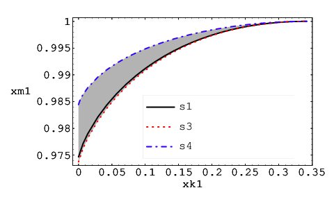
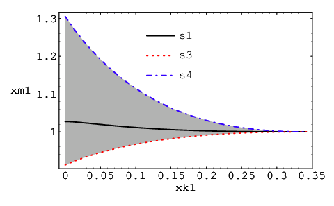
Trenutno ne poznamo zanesljivih ocen velikosti in , ki nastopata v formulah za kiralno ekstrapolacijo, ko upoštevamo prispevke stanj pozitivne parnosti. Zato njune možne prispevke ocenimo tako, da njuni vrednosti variiramo glede na vrednost med in . Opazimo, da so prispevki stanj pozitivne parnosti h kiralni ekstrapolaciji funkcije Isgur-Wise pod skalo majhni (okrog enega odstotka po naši oceni). Podobno splošno obnašanje lahko pripišemo funkciji ob zamenjavi , in . Tudi kiralna ekstrapolacija vrednosti (skupaj z popravki) deluje zelo položno in nakazuje, da je linearna ekstrapolacija v tem primeru lahko dober približek. Po drugi strani pa so potencialni prispevki h kiralni ekstrapolaciji odvoda po trenutnih grobih ocenah lahko precejšnji, do .
Naši rezultati so še posebej pomembni za izluščenje oblikovnih funkcij s pomočjo QCD na mreži. Trenutne napake na parameter v ekskluzivnih kanalih so že reda le nekaj odstotkov. To zahteva zelo natančen nadzor nad teoretičnimi napakami, ki lahko vplivajo na njegovo določitev. Razumevanje kiralnih popravkov je bistveno za zagotavljanje verodostojnosti izluščenja oblikovnih funkcij in ocene napak na mreži. Naše ocene vodilnih popravkov postavljajo mejo na natančnost takšnih ekstrapolacij.
Mešanje težkih nevtralnih mezonov
Oscilacije v sistemih mezonov posredujejo nevtralni tokovi, ki spreminjajo okus. Znotraj SM so prepovedane na drevesnem nivoju, zato nam njihove meritve omogočajo dostop do delcev znotraj relevantnih zančnih diagramov. Dandanes se natančno merjene vrednosti [56], in [57] uporabljajo za omejitev oblike unitarnostnega trikotnika CKM in tako določajo količino kršitev CP znotraj SM [3, 4]. Cilj nam otežujejo teoretične napake v izračunih vrednosti razpadnih konstant in parametrov “vreče” (ang. bag parameters) . Te količine lahko v principu izračunamo na mreži. Veliko oviro pri tem pa predstavlja majhna masa kvarka , ki je v simulacijah ne moremo doseči neposredno, temveč le preko kiralne ekstrapolacije. Oglejmo si torej vplive težko-lahkih mezonov pozitivne parnosti na izračun kiralnih popravkov razpadnih konstant in parametrov vreče, ki nastopajo v študijah prispevkov SM in supersimetričnega SM k mešalnim amplitudam .
Prispevki supersimetričnega SM k mešalni amplitudi se ponavadi obravnava v tako imenovani supersimetrični bazi operatorjev [58]:
| (29) | |||||
kjer sta in barvna indeksa. Znotraj SM k mešalni amplitudi pomembno prispeva le operator . Matrični elementi gornjih operatorjev so ponavadi parametrizirani s pomočjo parametrov vreče , ki predstavljajo merilo odstopanja od približka VSA
| (30) |
kjer smo z označili skalo renormalizacije, pri kateri ločimo nizko od visokoenergijskih prispevkov k amplitudam.
Za opis nizkoenergijskega obnašanja matričnih elementov operatorjev (Mešanje težkih nevtralnih mezonov) uporabimo HMPT. Preden se podamo v podrobnosti naj omenimo, da obstaja v eksaktni limiti statičnih težkih kvarkov (v tej limiti bomo operatorje označevali s tildo) zveza med operatorji (Mešanje težkih nevtralnih mezonov), in sicer , ki nam omogoča, da iz obravnave izločimo enega izmed njih. V isti limiti definiramo tudi razpadne konstante težko-lahkih mezonov namreč kot
| (31) |
kjer smo z in označili aksialni in psevdoskalarni tok. Nazadnje upoštevamo še izsledke študije kiralnih popravkov v kaonski fiziki [59], po katerih se operatorja in razlikujeta le po barvnih indeksih – lokalni izmenjavi gluona, ki pa ne more vplivati na nizkoenergijske lastnosti amplitud. Ta dva operatorja morata torej utrpeti identične kiralne popravke. Tako nam za analizo kiralnih popravkov ostanejo le trije matrični elementi operatorjev: , in , ki jih s polji HMPT zapišemo kot
| (32) | |||||
kjer smo označili .
Najprej se osredotočimo na kiralne popravke k (psevdoskalarnim) razpadnim konstantam težkih mezonov. Prispevke dobimo iz zančnih diagramov na sliki 11.
Diagram na desni prispeva le v teoriji s težko-lahkimi mezoni obeh parnosti, saj lahko znotraj zanke tečejo le (psevdo)skalarni mezoni. Izračuni popravkov na podlagi teh diagramov ponovno pokažejo, da prisotnost stanj pozitivne parnosti ne prizadane pionskih popravkov k razpadni konstanti, se pa popravki teh stanj kosajo s kaonskimi in eta popravki. Relavantni kiralni logaritemski popravki tako ponovno prihajajo iz teorije s simetrijo in jih lahko zapišemo kot
| (33) |
kjer smo z označili relevantne kontračlene. Hkrati lahko enostavno preverimo, da so kiralni popravki k skalarni razpadni konstanti težko-lahkih mezonov identični, z zamenjavo sklopitev in
| (34) |
Kot smo že pokazali v prejšnjih razdelkih, velja , zato pričakujemo da bodo odstopanja od linearne ekstrapolacije za manjša kot za .
Končno se posvetimo mešalnim amplitudam, ki dobijo kiralne popravke iz diagramov na sliki 12.
Ponovno diagrami v spodnjih dveh vrsticah prispevajo le ob upoštevanju težko-lahkih stanj obeh parnosti. Osredotočimo se na območje in postopamo podobno kot doslej. Zančne integrale namreč razvijemo po obratnih potencah masne reže med težko-lahkimi mezoni obeh parnosti in ponovno pokažemo, da ostanejo vodilni pionski logaritemski popravki neprizadeti in kiralna ektrapolacija znotraj teorije dobro definirana. Zapišemo
| (35a) | |||||
| (35b) | |||||
kjer smo označili , in .
Morda je na tem mestu dobro povdariti, da je diskusija tega razdelka pomembna predvsem tudi za fenomenološke pristope, ki označujejo logaritemske popravke kaonov in et kot napovedi in hkrati določijo relevantne kontračlene iz limite velikega števila barv ali kakšnega drugega modela. Pokazali smo namreč, da so prispevki blizu ležečih skalarnih resonanc po velikosti konkurenčni prispevkom kaonov in et, ter jih zato v takšnih diskusijah ne moremo zanemariti ali iz njih izločiti. Vendar pa je dejstvo, da bližnja skalarna stanja ne pokvarijo poglavitnih pionskih logaritemskih prispevkov, zelo dobrodošlo za študije QCD na mreži, saj lahko te še vedno uporabljajo formule HMPT za ektrapolacijo njihovih rezultatov. Takšni postopki pa morajo biti omejeni na teorijo in pod skalo .
Izračunali smo torej vodilne kiralne popravke k celotni bazi supersimetričnih operatorjev, ki prispevajo k mešanju težkih nevtralnih mezonov. Pokazali smo, da bližnje skalarne resonance ne vplivajo na vodilne pionske logaritemske prispevke, ki zato ostajajo zanesljivo vodilo pri kiralnih ektrapolacijah rezultatov simulacij na mreži. Hkrati smo preverili, da se vodilni kiralni popravki k razpadnim konstantam težko-lahkih mezonov sode in lihe parnosti ujemajo ob zamenjavi efektivnih sklopitvenih konstant .
Redki hadronski razpadi in mezonov
Redki razpadi mezonov veljajo za eno najobetavnejših področij za odkritje nove fizike izven SM [60, 61, 62]. Pričakovati je namreč, da bodo novi virtualni delci vplivali na te procese. To še posebej velja za razpade, ki potekajo preko nevtralnih tokov, ki spreminjajo okus, saj ti znotraj SM potekajo le preko zank. Ekstremni primer kašnega pristopa je iskanje razpadov, ki so znotraj SM izredno redki, in že samo opažanje katerih bi pomenilo jasen signal nove fizike. Huitu, Lu, Singer in Zhang so pred leti predlagali razpade in (v katerih se čudnost spremeni za oz. ) [63, 64] kot prototipne v takšnem iskanju. Njihov predlog temelji na dejstvu, da so takšni razpadi znotraj SM izredno redki, saj potekajo preko izmenjave gornjih kvarkov in bozonov znotraj škatlastih zank in imajo posledično razvejitvena razmerja reda do .
Prihajajoči pospeševalnik LHC bo med drugim izredno produktivna tovarna mezonov , Pričakovanja za njihovo proizvodnjo se namreč gibljejo okoli dogodkov na leto ob luminoznosti [65]. Četudi bi bila dejanska številka nekaj redov velikosti manjša, bo omogočala študij redkih razpadov mezonov , ki bo morda osvetlil prispevke fizike izven SM. Posvetili se bomo torej izračunom redkih prehodov in v dvo- in trodelčnih razpadnih kanalih mezona znotraj SM ter nekaj najpopularnejših okvirov nove fizike. Na podlagi znanih eksperimentalnih omejitev na prispevke obravnavanih modelov bomo podali napovedi za razvejitvena razmerja ter identificirali najperspektivnejše kanale za iskanje signalov nove fizike.
Efektivni šibki Hamiltonov operator, ki zaobjema tudi procese in zapišemo kot
| (36) |
kjer in označujeta efektivne Wilsonove sklopitve, s katerimi pomnožimo celotno bazo operatorjev, ki prispevajo k procesom (za ) in (za ). Izberemo
| (37) |
skupaj z dodatnimi operatorji , ki jih dobimo s primernimi kiralnimi transformacijami gornjih (), ter vse skupaj še z obrnjenimi okusi kvarkov in .
Znotraj SM k procesu () prispevata le operatorja . Glavne prispevke k Wilsonovim sklopitvam dajo top in čarobni kvarki ter bozoni znotraj škatlastih zank
| (38a) | |||||
| (38b) | |||||
kjer je
| (39a) | |||||
| (39b) | |||||
Z uporabo numeričnih vrednosti matričnih elementov CKM iz PDG [52] lahko postavimo mejo in .
Obravnavamo tudi prispevke nekaterih modelov fizike izven SM: minimalni supersimetrični SM (MSSM) z in brez parnosti R (RPV) ter model z generičnim dodatnim vektorskim bozonom . Znotraj MSSM prispevata, podobno kot v SM, le operatorja , medtem ko sta pripadajoča Wilsonova koeficienta iz izmenjave parov gluinov () in spodnjih skvarkov () [58]
| (40a) | |||||
| (40b) | |||||
kjer sta
| (41a) | |||
| (41b) | |||
in smo definirali . Z uporabo obstoječih mej na parametre MSSM (, , ) iz študij oscilacij mezono , in ter drugih redkih razpadov mezonov in lahko spet omejimo vrednosti in . V primeru, da znotraj MSSM dopustimo interakcije tipa RPV, dobimo poglavitne prispevke že v drevesnem redu preko izmenjave snevtrinov (). K efektivnemu Hamiltonovemu operatorju potem prispevajo predvsem operatorji in z Wilsonovimi sklopitvami
Obstoječe študije ne omejujejo vseh parametrov (, ), ki nastopajo v teh procesih, zato bomo omejitve podali iz napovedi za merjene ekskluzivne razpadne kanale.
Mnoge razširitve SM vsebujejo dodatne nevtralne vektorske bozone [66, 67]. Ti lahko prispevajo k efektivnemu Hamiltonovemu operatorju v drevesnem redu preko operatorjev ter tudi . Pripadajoče Wilsonove koeficiente lahko zapišemo kot
| (43) |
kjer je in . Z , , in smo označili umeritvene sklopitvene konstane in mase bozonov in , medtem ko označuje mešalni kot.
V izračunu pogostosti razpadnih kanalov mezona , ki potekajo preko kvarkovskih prehodov in moramo izvrednotiti matrične elemente efektivnih Hamiltonovih operatorjev med hadronskimi stanji. V prvem približku uporabimo popolno faktorizacijo oz. VSA, ki v večini primerov zadovoljivo opiše glavne lastnosti razpadnih kanalov, ki jih obravnavamo. Izjeme so kanali, v katerih razpadne amplitude v faktorizacijskem približku izginejo. O takšnih razpadih naša metoda molči; potrebni bi bili bolj natančni pristopi. Obravnavamo dvodelčne razpadne kanale , in , kot tudi trodelčne kanale , , , , , in . Pri tem uporabimo teoretične uvide iz hadronskih in semileptonskih študij težkih mezonov iz prejšnjih razdelkov, kot tudi iz drugih virov. Predvsem se izkaže pomebna vloga vmesnih resonanc pri modeliranju hadronskih oblikovnih funkcij, ki nastopajo v faktorizacijskem približku, pomagajo pa nam tudi natančno določene vrednosti nekaterih sklopitvenih konstant znotraj HMPT.
Na podlagi izračunanih amplitud za izbrane hadronske kanale, najprej omejimo proste parametre modelov RPV in , tako da naše napovedi primerjamo z obstoječimi eksperimentalnimi mejami na razvejtiveni razmerji razpadov in , ki so jih izmerili v eksperimentu Belle [68]. V primeru modela RPV normaliziramo mase snevtrinov na skupno masno skalo in dobljene meje zapišemo kot
| (44a) | |||||
| (44b) | |||||
Lahko pa predpostavimo, da poglavitni prispevki nove fizike prihajajo v obliki dodatnih bozonov . V tem primeru dobimo meje na njihove sklopitve oblike
| (45a) | ||||
| (45b) | ||||
in
| (46a) | ||||
| (46b) | ||||
Meje (44a-46b) so zanimive, predvsem ker omejujejo kombinacije parametrov RPV oz. , v ortogonalni smeri od obstoječih meritev oscilacij mezonov , , , ter drugih redkih procesov. Na podlagi teh omejitev lahko končno podamo tudi napovedi za razvejtivena razmerja mnogih možnih dvo- in trodelčnih razpadnih kanalov mezona . Naši rezultati so povzeti v tabeli 6.
| Razpad | SM | MSSM | RPV | |
|---|---|---|---|---|
Napovedi SM in MSSM so zanemerljivo majhne. Na podlagi omejitev na parametre RPV iz razpadnih kanalov in dobimo v tem modelu največja razvejtivena razmerja za trodelčne razpadne kanale in , ter dvodelčne razpadne kanale , , in . Poleg teh, pa znotraj modela dobimo velika razvejitvena razmerja še v kanalih in . Eksperimenti namesto mezonov ali , dejansko izmerijo stanja mezonov oz. . Posledično bo v razpadnih kanalih, ki vsebujejo nevtralne psevdoskalarne kaone, zaradi prispevkov pingvinskih diagramov znotraj SM težko zaznati vplive nove fizike [69]. V tem pogledu so bolj perspektivni razpadi v nabite kaone oziroma njihova vektorska stanja.
V našem izračunu smo se naslanjali na približek naivne faktorizacije, ki je kot prvi približek zadostna za opis grobih lastnosti prispevkov nove fizike. Tudi v primeru, da bi morebitni nefaktorizabilni prispevki znatno spremenili vrednosti hadronskih amplitud, je razkorak med napovedmi SM in nove fizike trenutno tolikšen, da v vsakem primeru ohranja relevantnost obravnavanih razpadnih kanalov v iskanju nove fizike, in to nemudoma, ko bodo na voljo večje količine mezonov .
Zaključki
Neperturbativna narava QCD je trdovraten problem računov v hadronski fiziki. Ena izmed njegovih manifestacij je pojav resonanc v hadronskem spektru. V procesih, kjer so izmenjane gibalne količine majhne v primerjavi s skalo zlomitve kiralne simetrije , lahko uporabimo pristop efektivnih teorij, ki temelji na približni kiralni simetriji lahkih kvarkov ter približni simetriji okusov in spina težkih kvarkov. V takšnem okviru lahko sistematično analiziramo vpliv najnižje ležečih resonanc v procesih težkih mezonov.
HMPT smo uporabili na primeru močnih, semileptonskih in redkih procesih težkih mezonov. V ogrodje efektivne teorije smo sistemtično vključili najnižje ležeče spinske multiplete težkih mezonov pozitivne in negativne parnosti.
V prvem redu kiralnega razvoja smo pokazali, da lahko bližnje ležeča vzbujena stanja težkih mezonov pomagajo razložiti nekatere lastnosti semileptonskih oblikovnih funkcij v razpadih težkih v lahke mezone. Namreč, z uporabo omejene parametrizacije oblikovnih funkcij, ki temelji na približnih limitah efektivnih teorij QCD, smo uspeli zasičiti prispevke celotnega stolpa vmesnih stanj samo z najbližje ležečimi stanji primernih kvantnih števil. Parametrizacijo smo napeli na izrčun razpadne širine v kinematskem območju majhnih izmenjav gibalne količine znotraj HMPT. Takšen model je uspešno reproduciral večino oblikovnih funkcij in prehodov znotraj trenutnih eksperimentalnih napak in v ujemanju z obstoječimi izračuni QCD na mreži.
V drugih procesih, ki smo jih obravnavali, prispevajo vzbujena stanja težkih mezonov šele v drugem redu kiralnega razvoja – k tako imenovanim kiralnim popravkom. Obravnavali smo močne razpade težkih mezonov ter izračunali efektivne močne sklopitvene konstante med pari težkih mezonov sode ali lihe parnosti ter lahkimi psevdoskalarnimi mezoni v drugem redu kiralnega razvoja. Iz merjenih razpadnih širin in smo izluščili efektivne sklopitvene konstante v prvem in drugem redu kiralnega razvoja. Vpliv velikega števila novih neznanih parametrov, ki nastopajo v izračunih drugega reda, smo ocenili s pomočjo variacij skale kiralne zlomitve ter otipanjem prostora parametrov ob prilagajanju izračunov na eksperimentalne meritve. Nato smo študirali ekstrapolacijo sklopitvenih konstant v limiti, ko gredo mase lahkih psevdoskalarnih mezonov proti nič. Ugotovili smo, da dajo naivni izračuni kiralnih popravkov z upoštevanjem vzbujenih težkih stanj slabo definirano kiralno limito. Namesto tega lahko izvedemo razvoj v obratni vrednosti masnih razlik med osnovnimi in vzbujenimi stanji težkih mezonov in tako rešimo kiralno limito izračunov. Takšen razvoj je zanesljiv za majhne mase lahkih psevdoskalarnih mezonov, manjše od masnih razlik med osnovnimi in vzbujenimi stanji težkih mezonov. Potem se prispevki vzbujenih stanj težkih mezonov formalno izražajo kot popravki višjih redov v kiralnem razvoju teorije brez dinamičnih vzbujenih stanj. Ti rezultati so še posebej pomembni za študije QCD na mreži, ki uporabljajo kiralno ektrapolacijo za dosego fizikalne limite simuliranih mas lahkih kvarkov. Po naših ugotovitvah je relevantna kiralna limita takih ektrapolacij izpospinska limita, zanesljivo pa se lahko izvedejo le za pionske mase manjše od masnih razlik med osnovnimi in vzbujenimi stanji težkih mezonov. Hkrati lahko ocenimo zanesljivost ektrapolacij takšne simetrije v redu vodilnih logaritmov z uporabo vodilnih prispevkov vzbujenih težkih stanj višjega reda.
Razklopitev vzbujenih resonanc in njihove poglavitne prispevke smo preverili tudi na primeru semileptonskih oblikovnih funkcij v težko-težkih prehodih med mezoni sode in lihe parnosti, kjer smo izračunali kiralne popravke k funkcijam Isgur-Wise. Za izluščenje matričnega elementa CKM namreč poleg izredno natančne določitve razpadnih širin iz eksperimentov in oblikovnih funkcij iz izračunov QCD na mreži potrebujemo natančno poznavanje kiralne limite. Ugotovili smo, da so efekti vzbujenih resonanc težkih mezonov primerljivi s trenutnimi ocenami teoretičnih napak in jih bo zato v prihodnjih študijah potrebno upoštevati.
Redke procese težkih mezonov analiziramo predvsem z namenom iskanja signalov nove fizike izven SM. Vendar pa lahko upamo na uspeh le ob dobrem poznavanju in nadzoru nad hadronskimi efekti. V ta namen smo obravnavali kiralno obnašanje celotne supersimetrične baze efektivnih operatorjev , ki so odgovorni za oscilacije nevtralnih težkih mezonov. Izračunali smo popravke kiralnih zank v drugem redu kiralnega in prvem redu razvoja po masah težkih kvarkov ter vključili vplive težkih mezonov sode parnosti. Potrdili smo razklopitev vzbujenih stanj in podali izraze za kiralno ekstrapolacijo celotne baze efektivnih operatorjev v redu vodilnih logaritmov. Naš rezultat bodo tako lahko uporabile prihodnje študije teh procesov s simulacijami QCD na mreži. Kot pomožni rezultat smo izračunali vodilne kiralne logaritemske popravke k razpadnim konstantam težkih mezonov sode parnosti.
Nazadnje smo izvrednotili zelo redke prehode in mezona v pristopu efektivnih teorij. Hadronske razpadne amplitude smo ocenili s pomočjo približkov faktorizacije in zasičenja z resonancami. Prehode smo analizirali znotraj večih modelov nove fizike. Na podlagi obstoječih eksperimentalnih mej na pogostosti razpadov in smo lahko omejili relevantne kombinacije parametrov nove fizike. Končno smo na podlagi teh omejitev identificirali najobetavnejše dvo- in trodelčne neleptonske razpade mezona , v katerih bi lahko s pomočjo prihodnjih delčnih trkalnikov iskali signale teh redkih prehodov.
Tekom računa smo razrešili tudi nekaj tehničnih podrobnosti. Morali smo izluščiti celoten nabor kontračlenov v drugem redu kiralnega razvoja, ki prispevajo k močnim prehodom med težkimi mezoni sode in lihe parnosti, ter lahkimi psevdoskalarnimi mezoni. Vključitev vzbujenih stanj težkih mezonov je nato pokvarila kiralno limito izračunov v redu vodilnih logaritmov. Problem smo razrešili s pomočjo odrezanega razvoja zančnih integralov po obratni vrednosti masnih razlik med osnovnimi in vzbujenimi stanji težkih mezonov, na račun zmanjšanja intervala zanesljivosti izračunov znotraj HMPT. V primeru semileptonskih prehodov med težkimi in lahkimi mezoni smo morali pravilno reproducirati limiti HQET in SCET, da smo lahko dobili veljavno parametrizacijo oblikovnih funkcij. Hkrati smo morali med seboj pravilno napeti bazi oblikovnih funkcij znotraj QCD in HQET, ter identificirati prispevke izračunov znotraj HMPT k posamičnim oblikovnim funkcijam. Ugotovili smo, da le takšno pravilno napenjanje oblikovnih funkcij verno reproducira prispevke resonanc pravilnih kvantnih števil k oblikovnim funkcijam. Nenazadnje smo morali zaradi strukture polov v parametrizaciji oblikovnih funkcij v naše HMPT izračune vključiti prispevke radialno vzbujenih stanj težkih mezonov. V izračunih kiralnih popravkov k mešanju težkih nevtralnih mezonov smo morali predpisati pravilen postopek bozonizacije efektivnih operatorjev. Izkazalo se je, da je mogoče ogromen nabor vseh možnih struktur znotraj HMPT s pomočjo spinske simetrije težkih kvarkov in identitet matrik znantno skrčiti. Podobno smo morali na primeru prehodov in identificirati celotno bazo kvarkovskih operatorjev, kot tudi njihov tok in mešanje v prvem redu enačb renormalizacijske grupe. Le tako smo lahko ohranili nadzor nad vodilnimi popravki QCD v visokoenergijskem režimu. Nenazadnje smo za oceno mnogih hadronskih amplitud v dvo- in trodelčnih razpadih mezona morali izvesti vhodne HMPT izračune ter po potrebi vključiti tudi prispevke lahkih vektorskih ter skalarnih resonanc. Ob tem smo smiselne fenomenološke rezultate dobili le s pravilnimo predpisanimi postopki resonančnega zasičenja amplitud.
Chapter 1 Introduction
The Standard Model (SM) of elementary particle physics is a quantum gauge-field theoretical description of fundamental electromagnetic, weak and strong interactions. It emerged in the 1960’s and has completely dominated the field ever since [1]. The building blocks of the SM are fermions -- leptons and quarks -- which come in three families. The SM gauge group is , where the is the gauge group of Quantum Chromodynamics (QCD), is the gauge group of weak isospin, while is the gauge group of weak hypercharge. Only the left-handed chiral fermions transform as weak isospin doublets under the , while quarks also form the fundamental triplet representation of . The masses of leptons and quarks are generated via the Higgs mechanism -- spontaneous symmetry breaking, where the (chiral) symmetry of the theory is not respected by the vacuum. For this purpose an additional scalar weak isospin doublet is introduced. Its vacuum expectation value also breaks gauge invariance of the theory to the subgroup , inducing masses for the weak and gauge bosons.
The quark fields in the basis are not the mass eigenstates in general. Therefore it is customary to rotate them to the mass eigenbasis by means of a unitary matrix. The rotation is conventionally conveyed to the down-quark fields and the rotation matrix is called the Cabibbo-Kobayashi-Maskawa (CKM) matrix. It can be fully described by three real mixing angles and a complex CP violating phase.
The successes of the SM description are abundant. Its predictions have been extensively tested in accelerator facilities and agree well with the data measured up to energies available at present: the electroweak precision tests are generally in impressive agreement with SM predictions [2] while the CP violation experiments in , and meson systems support the CKM description with one universal phase [3, 4]. The only elementary building block presently lacking experimental detection is the Higgs boson.
However we also know from observations, that the SM cannot be the ultimate fundamental theory. For once, it does not include gravity. Although colossal theoretical efforts have been spent on the subject in the last few decades, the progress has been slow and the results inconclusive. Mainly also due to the lack of almost any experimental hints in the area. On the other hand, the SM also does not account for the recently measured neutrino oscillations [5]. Explanation of these requires non-zero neutrino masses, contrary to the SM prescription11 1 In fact, the matter contents of the SM can easily be extended to include right-handed neutrinos and thus allowing for Dirac neutrino masses via the Higgs mechanism. However the observed smallness of the neutrino masses and the fact that right-handed neutrinos must be singlets under the SM gauge group seem to prefer alternative mechanisms which lie beyond the SM.. Thirdly, a growing number of astrophysical observations suggest that most of the matter in the universe is neither luminous nor baryonic [6]. In addition, most of it must be slowly moving or ‘‘cold’’. The SM does not provide a candidate for nonbaryonic cold dark matter. Finally, our current understanding of baryogenessis -- the generation of the measured baryon - antibaryon asymmetry -- in the early universe requires levels of CP and baryon number violation much higher than allowed for in the SM [7].
There are also some conceptual and ‘‘aesthetic’’ problems with the SM. The running of the gauge couplings suggests a unification scale at although precise unification does not occur if one takes into account only SM fields [70]. Neither does the SM describe the dynamics of such unification. In fact, even the electroweak symmetry breaking has no dynamical explanation within the SM. It is imposed by construction and renders the masses of the elementary particles as free parameters. Compared to the large unification scale the electroweak scale also appears to be very small. The large scale hierarchy manifests itself in form of large quantum corrections to the mass of the Higgs boson, which are quadratically divergent and thus sensitive to the UV completion of the theory22 2 This has to be compared to the logarithmic divergences of fermionic fields due to chiral symmetries and gauge boson fields due to gauge invariance.. Even more appealing is the “fine-tuning” required for the vacuum energy density when compared to the measured present critical density of the universe [6]. Its classical value, which is a free parameter in any quantum field theory (QFT), has to cancel corrections due to spontaneous symmetry breaking and the resulting vacuum condensates in the SM at energy scales from a few to a few . Another similar issue is related to the strong CP phase of the QCD vacuum. Its value, a free parameter of the SM, is severely constrained by the measurements of the electric dipole moment of the neutron [1].
All of these reasons call for physics beyond SM, and many proposals exist on what the physical reality ought to look like above the electroweak scale. For example, supersymmetric (SUSY) extensions of the SM attempt to resolve the Higgs hierarchy problem and provide suitable dark matter candidates [71, 72]. The simplest and most studied of these is the Minimal SUSY SM (MSSM) which adds a bosonic partner to each SM fermion and a fermionic counterpart to each boson, but also doubles the Higgs sector. Possible alternative proposals come in the form of (large) extra-dimensions in which some or all of the SM fields may propagate or extended SM symmetries. In order for any of these extensions to address the dynamics at the electroweak scale, new physical degrees of freedom have to appear at the TeV scale. On the other hand, many of these ‘‘low scale’’ new physics scenarios can be embedded into high scale unification theories, such as Grand Unified Theories (GUTs) attempting to describe the unification of the SM couplings at large scales in terms of incorporating the SM gauge group into larger symmetries [73]. Even more ambitious are the various String theories unified under the name of M-theory, which also attempt to address the quantization of gravity and the cosmological evolution of the very early universe [74, 75]. In order to get a handle on this plethora of high energy phenomenologies one must often rely on the so-called ‘‘bottom-up’’ approach to new physics. One constructs effective low energy theories by systematically parameterizing possible new physics contributions to low energy processes based on symmetry principles of the expected underlying theory. Within this framework, the SM itself is regarded as an effective low energy description of a grander theory, containing the SM particle content and gauge symmetry at low energies. A similar reasoning lies behind the MSSM, which is often regarded as the low energy effective theory of a high scale (and/or dimensional) GUT or String theory, containing a (slightly broken) SUSY SM particle content at energies close to the electroweak scale. Alternatively, one can focus on specific low energy aspects, common to various SM extensions. A common characteristic of various new physics models (including MSSM) is the appearance of a doubling of the Higgs sector, which can be put in the general form of a Two Higgs Doublet Model (THDM). On the other hand many GUT and String theories also predict additional low energy gauge extensions to the SM – the appearance of additional bosons. By focusing on such common aspects, one can extract important general signatures of various new physics proposals.
The experimental challenge of finding new physics follows two main directions. In direct searches the idea is to produce the new particles and detect them directly (often through their decay products). This requires high enough energies at particle colliders such as the Tevatron, the upcoming LHC or the planned ILC. A complementary idea is to measure the effects of new particles in processes where they enter as intermediate virtual states. In this approach it is crucial to be able to disentangle the effects of new physics from those conveyed by the SM particles. One may then employ the “top-down” approach as prototyped by the Wilsonian Operator Product Expansion (OPE) [76]. Namely one may represent low energy Green’s functions or scattering amplitudes in terms of products of local operators, which are in term computed (matched to) the full original formulation of the SM and possible additional higher energy extensions. In this way SM and new physics contributions are clearly separated on an amplitude-by-amplitude basis. The task is then to compute low energy scattering cross sections and decay rates and compare them to precision measurements. This approach both tests SM predictions as well as probes possible new physics contributions. Experimentally it requires high statistics and precision measurements, such as those provided in the last years by the B and D meson factories at Belle, BaBar, CLEO-c and others. Among their successes are the by now established neutral meson oscillations in all neutral [1], [77, 78], [56] and [57, 79] meson systems, as well as ever tightening consistency constraints on the CKM unitarity and the CP violating phase. So far, no clear indications of new physics in these phenomena have been observed and several stringent experimental bounds on various new physics proposals have been imposed.
In order to correctly interpret experimental results and justify the consistency with the SM or claim new physics signals, one first has to reliably calculate the relevant hadronic processes based on the quark picture of the OPE. Due to the nonperturbative and confining nature of low energy QCD, this turns out to be a daunting task. Namely, the expansion in the coupling constant is not applicable in this regime. Ab initio calculations, i.e., by starting with the QCD Lagrangian and finishing up with predictions for physical observables are still possible, through the use Lattice QCD techniques, but are computationally very challenging [8]. Lattice methods also have their own limitations. To get meaningful results, computations have to be done in Euclidean space-time, which makes calculations of processes with more than one hadron in the final state very difficult. Also, in order to make numerical difficulties tractable, a number of approximations have to be made, e.g., by working at relatively large pion masses. Another option that has been commonly used in the past, is to use symmetries of the QCD Lagrangian to construct effective theories [9]. Unknown parameters in the effective theory are fixed from experiments or, if possible, from perturbative comparison (matching) to full QCD. These effective theories may then be employed to either predict some experimental processes directly, or to assist nonperturbative Lattice QCD calculations making them more tractable and keeping control of the used approximations.
One important manifestation of the strong QCD dynamics at low energies is the appearance of resonances in the particle spectrum. They have been detected long ago and studied extensively in the processes of pions and kaons [1]. Their effects proved to be critical in many low energy processes. On one hand they restrict the validity of effective theory approaches, which are not able to fully include their effects, e.g., in (resonant) scattering. Also, their dominant (long distance) effects are known to almost completely obscure contributions due to (short distance) SM OPE or possible new physics contributions in meson oscillations and rare decays [10]. On the other hand, due to the relatively large and quark masses, heavy meson resonance effects were long believed to be less significant in processes among hadrons involving these two quarks.
In the last couple of years however, many experiments have reported first observations of resonances in the charm spectrum. In 2003, Belle [11] and FOCUS [12] experiments reported the observation of broad resonances and , ca. higher above the usual states and with opposite parity. In the same year BaBar [13] announced a narrow meson . This was confirmed by FOCUS [14] and CLEO [15] which also noticed another narrow state, . Both states were also confirmed by Belle [16]. The basic properties of the relevant charmed mesons together with the dominating hadronic decay modes are listed in table 1.1.
| Meson | Mass | Width | (final states) | |
| , | ||||
| [12] | 33 3 Observed channel. | |||
| 44 4 Average of Belle [11] and FOCUS [12] values from [80]. | 44 4 Average of Belle [11] and FOCUS [12] values from [80]. | 33 3 Observed channel. | ||
| 55 5 Average of Belle [11] and CLEO [81] values from [80]. | 55 5 Average of Belle [11] and CLEO [81] values from [80]. | 33 3 Observed channel. | ||
| 33 3 Observed channel. | ||||
| 33 3 Observed channel. | ||||
Studies of the basic properties of these states have been triggered particularly by the fact that the and states’ masses are below threshold for the decay into ground state charmed mesons and kaons, as suggested by quark model studies [17, 18] and lattice calculations [19, 20]. Their relative closeness to the ground state charmed mesons suggests possibly significant effects in the processes of the lowest and states and poses the following questions: Can we estimate the relevant effects of the lowest heavy meson resonances to the processes of heavy meson ground states? Can we keep their effects under control, especially within effective theories of QCD? Can they possibly help us to understand certain aspects of observed and measured ground state heavy meson processes? And finally what conclusions, drawn for the charm sector can we apply to the processes of and mesons, whose resonances are currently still beyond the reach of experimental facilities66 6 During the final stages of preparation of this thesis D0 collaboration has reported the first observation of axial resonances in the spectrum [82]. Their properties and interpretation are yet to be analyzed in detail..
In this thesis we will explore several aspects of resonances in the heavy meson processes [21, 22, 23, 24, 25, 26, 27, 28, 29]. Their leading order contributions, either at tree level or at one loop, will be analyzed in the relevant effective theory approach to QCD. Within this framework we will calculate hadronic parameters entering various low energy processes and study the impact of heavy meson resonances on observables. These include strong, semileptonic decay rates of heavy mesons as well as neutral heavy meson mixing parameters. Since strong decay channels, if open, usually dominate the measured decay widths, one may use these as benchmarks on the validity of the chosen effective theory approach and also determine from them basic parameters of the effective theory. Semileptonic decays, mediated by quark and charged lepton weak currents proceed at tree level in the SM and are confirmed to be dominated by SM contributions. Their detailed study may therefore produce important consistency checks within the SM, such as the determination of the various CKM matrix elements and testing its unitarity, provided the relevant hadronic effects are well understood. Heavy neutral meson mixing, on the other hand, is mediated by box diagrams in the SM. This makes it an important arena for studying possible new physics contributions, which may or may not be suppressed by loop factors. Within our approach we will analyze all possible hadronic amplitudes entering heavy neutral meson mixing within the SM or beyond. Finally, we will also analyze very rare hadronic decays of the doubly heavy meson, which are, like the neutral meson mixing, mediated by box diagrams in the SM. There we will make use of some of the knowledge on the impact of resonances in the calculation of the relevant hadronic decay amplitudes in order to constrain various new physics proposals based on existing experimental searches and also propose prospecting new search directions.
The outline of the thesis is as follows. In the first two chapters we introduce the prerequisites for the phenomenological studies in the subsequent chapters. In chapter 2 we introduce the concept of effective field theories with a focus on the effective theory approaches to QCD in the limits of small and large quark masses. In chapter 3 we review some commonly used tools in hadronic calculations, such as the OPE, general hadronic matrix element parameterizations, and some of their approximations. In chapter 4 we analyze strong decays of heavy mesons within an effective theory approach, including loop contributions of excited heavy meson resonances. We attempt to extract the relevant effective strong meson couplings from the measured decay rates and study the impact of the resonances on the coupling extraction from Lattice QCD calculations. In chapter 5 we analyze the leading contributions of the heavy meson resonances to semileptonic decays. Both heavy to light as well as heavy to heavy meson transitions are analyzed. While in the former, heavy resonances may contribute already at tree level, in the latter their contributions are loop suppressed. Similar, loop suppressed contributions to heavy neutral meson mixing hadronic amplitudes are studied in chapter 6. Finally, chapter 7 contains our analysis of the very rare hadronic decays of the meson within the SM and some of its extensions. The conclusions are gathered in Chapter 6, while some further technicalities of our calculations as well as brief descriptions of studied SM extensions are relegated to the appendices.
Chapter 2 Effective theories of heavy and light quarks
2.1 What is an effective field theory?
The content of quantum theory is encoded in its Green’s functions, which in general depend in a complicated way on the properties (e.g. particle momenta) of the initial and final states. In particular they exhibit nonanalytic behavior such as cuts and poles in the configuration variables, which arise when the kinematics allow for physical intermediate states. Conversely, when the kinematics are far from being able to produce a certain propagating intermediate state, the contribution of that state to the Green’s function of interest will be relatively simple, well approximated by the first few terms in a Taylor expansion (e.g. of the incoming momenta of the scattering problem). Instead of Taylor expanding each amplitude it turns out to be much more profitable to expand the Lagrangian in local operators that only involve the light degrees of freedom, where the expansion is in the powers of the generalized momenta of the light fields (appearing as derivatives in the Lagrangian) divided by the scale of heavy physics. Such a Lagrangian is called an effective field theory. Although the heavy modes do not appear explicitly anymore, their contributions are encoded through the parameters of the effective theory11 1 This aspect of effective theories is not unique to quantum phenomena. Integrating out certain regions or scales of the phase space in order to simplify the description of certain phenomena has also been found to be of high value in other fields such as (classical) statistical mechanics or (classical) field theories.. There are many situations in which effective field theories are of utility [83]:
- •
They allow one to compute low energy scattering amplitudes without having a detailed understanding of the short distance physics, or to avoid wasting effort calculating tiny effects from known short distance physics (such is the OPE and the effective weak Hamiltonian).
- •
In nonperturbative theories (such as low energy QCD) one can construct a predictive effective field theory for low energy phenomena by combining power counting of operators with symmetry constraints of the underlying theory (such as the PT and HMPT).
- •
By regarding theories of known physics as effective field theory descriptions of more fundamental underlying physics, one can work bottom up, extrapolating from observed rare processes to a more complete theory of short distance physics (this approach is taken in many studies of BSM physics, such as MFV or grand unification).
At present, the general approach of effective field theory is followed in many contexts of the SM and even in more speculative theories like grand unification, supergravity, extra dimensions or superstrings.
2.2 Exploring the Chiral symmetry of QCD
One of the earliest and also one of the most successful examples of effective theories is the chiral perturbation theory (PT) which builds upon the approximate chiral symmetry of QCD at low energies. We will briefly review it in this section. The QCD Lagrangian with () massless quarks
| (2.1) | |||||
where is the QCD covariant derivative and , has a global symmetry
| (2.2) |
At the effective hadronic level, the quark number symmetry is realized as baryon number. The axial is anomalous and is broken by nonperturbative effects. Theoretical and phenomenological evidence suggests that the chiral group on the other hand is spontaneously broken to the vector subgroup . The axial generators of are realized non-linearly and associated with them are the massless pseudoscalar Goldstone bosons parameterizing the right coset space. Here are the broken generators of and are the Goldstone fields. For the case, the can be written as
| (2.3) |
while in the only the pion fields remain. To preserve all the symmetries of the fundamental theory in the effective Lagrangian, it is essential to construct it out of the Goldstone field functions which transform linearly under (see e.g. [84] for details). A customary choice is , which transforms as , where and are the corresponding generators and respectively. is an undetermined constant of energy dimension one, which can be identified with the Goldstone boson decay constant. We continue by factoring out the broken generators of from the quark fields , where transforms under as . Here is the transformed Goldstone matrix and we demand that be an element of . In general it will also be a function of . Consequently, transforms as and we have to modify its covariant derivative to account for the coordinate dependence where the vector field and transforming as . It can be easily checked that transforms under as . There exists another operator which can be built up of , has the properties of an axial vector field and is transforming under as . Its role will become apparent later.
The Lagrangian of the SM is not chiral invariant. The chiral symmetry of the strong interactions is broken by the electroweak interactions generating in particular non-zero quark masses. The basic assumption of PT is that the chiral limit constitutes a realistic starting point for a systematic expansion in chiral symmetry breaking interactions. Namely we extend the chiral invariant QCD Lagrangian (2.1) by coupling the quarks to external hermitian matrix fields , , , [9]:
| (2.4) |
Here and will contain external photons and weak gauge bosons so that Green’s functions for electromagnetic and semileptonic weak currents can be obtained as functional derivatives of the generating functional with respect to external photon and weak boson fields. The scalar and pseudoscalar fields , on the other hand give rise to Green’s functions of (pseudo)scalar quark currents, as well as providing a very convenient way of incorporating explicit chiral symmetry breaking through the quark masses. To preserve the manifest chiral symmetry of the effective Lagrangian, we promote it to a local symmetry and treat the external fields as spurions with the transformation properties , and . Accordingly we have to introduce the covariant derivatives for pion fields (as well as the appropriate external field stress-energy tensors). The physically interesting Green’s functions are then functional derivatives of the generating functional at chosen values of the spurion fields. In particular for the quark masses we use . Even more generally, any effective quark operator (e.g. from the OPE of the effective weak Hamiltonian ) can be incorporated into the effective chiral Lagrangian by coupling it to the appropriate external chiral spurion field and then constructing the corresponding source terms out of the Goldstone fields.
The effective chiral Lagrangian is usually organized in a derivative expansion based on the chiral power counting rules. One prescribes chiral powers to all the constituent field operators and then builds the Lagrangian out of them by constructing all the terms adherent to the symmetries up to a given chiral power. In general, this procedure counts the powers of derivatives on the Goldstone fields as well as the number of external field insertions which at the level of Green’s functions translates to counting the powers of pseudo-Goldstone masses and exchanged momenta. Using the simplest choice for the quark mass chiral counting one arrives at the lowest order Lagrangian describing the low energy strong interactions of light pseudoscalar mesons [1, 30]
| (2.5) |
A trace is taken over the repeated light quark flavor indices. For the sake of clarity we have omitted all external currents () except in the second term, which induces masses of the pseudo-Goldstone bosons . While the normalization of the first term is canonical, the second term contains an unknown constant , which we can fit to the light pseudoscalar meson masses. Conversely, lattice QCD simulations often work in the exact flavor isospin symmetry limit. There, one can parameterize the pseudo-Goldstone masses according to the Gell-Mann formulae as [31]
| (2.6) |
where and .
Higher order terms in the chiral power counting can be constructed in this manner as well as terms involving any general external fields. The higher order terms in this expansion also serve a double role as the counterterms absorbing loop divergences from diagrams with insertions of lower order terms in the Lagrangian, thus keeping the theory renormalizable (in the general sense of the word).
2.2.1 Light flavor singlet mixing and the
The eight pseudo-Goldstone bosons: , , , , , , and have the same quantum numbers as the following quark-antiquark pairs: , , , , , , and . This suggests the existence of a ninth meson that would correspond to the singlet as the pseudo-Goldstone boson of the axial symmetry of QCD. However, due to the axial anomaly, the mass of is not protected and can be much larger than those of the other eight states.
Nevertheless, for practical reasons still has to be incorporated into the theory. Namely, its existence would entail mixing with the state to form two distinct physical states ( and ) and this scenario needs to be taken into account. One of the common approaches is to pretend that there is no axial anomaly and add to the matrix (2.3) as an singlet:
| (2.7) |
The mixing of and to form physical states can in principle involve other states (e.g. or even ), can depend on the energy of the state or can be influenced by the axial anomaly. Consequently the mixing scheme can be very complicated. In this thesis, we use the approach developed by Feldman et al. [85]. There, the physical states and can be written as linear combinations of and : , , where has a flavor structure and is an state, while is the mixing angle.
The decay constants of and follow the same pattern of state mixing:
| (2.8) |
with the decay constants defined as
| (2.9) |
Due to the flavor symmetry breaking effects and the axial anomaly . In the first order of flavor symmetry breaking, it can be deduced that , . Therefore, if the – basis is used instead, two mixing angles rather than one are needed , . The angles and are connected with , and as , .
The value of can be obtained phenomenologically from the various measured processes involving and states. The value that fits the data best is .
2.3 Symmetries of heavy quarks
Since their early applications, symmetries of heavy quarks have been one of the key ingredients in the theoretical investigations of processes involving heavy quarks. They have been successfully applied to the heavy hadron spectroscopy, to the inclusive as well as a number of exclusive decays (for reviews of the heavy quark effective theory and related issues see [86, 33]).
The important observation here is that for heavy enough quarks, the effective strong coupling of QCD, due to its renormalization group running and asymptotic freedom, will be small at the mass scale of the heavy quark. This implies that on length scales, comparable to the compton wavelength , the strong interactions are perturbative and much like the electromagnetic interactions. Furthermore, heavy quark spin participates in the strong interactions only through relativistic chromomagnetic effects. Since these vanish in the limit of the infinite quark mass, the spin of the heavy quarks decouples as well. The resulting theory therefore contains an approximate spin symmetry with the spin states of the heavy quark transforming in the fundamental representation. To arrive at this result formally, we start with the QCD Lagrangian for a single flavor of heavy quarks
| (2.10) |
We separate the quark fields into their positive and negative frequency parts – i.e. into ”quark” and ”anti-quark” fields , where annihilates the quark while creates the corresponding anti-quark. For an infinitely heavy (anti)quark field travelling with velocity , it is useful to rescale the ground state energy of the effective theory Fock space relative to the mass of the heavy (anti)quark in the frame of reference. This is done by factoring out the dominant kinetic phase factor from the (anti)quark fields . Then we further project out the large components of the heavy (anti)quark spinors using a velocity dependent projection operators to obtain the effective heavy (anti)quark fields . They satisfy . We construct the HQET Lagrangian from QCD by using the combined field while its orthogonal small (anti)quark spinor components can be integrated out using their equations of motions [87] or more elegantly via direct Gaussian path integration of the generating functional , where external sources only couple to the fields and none to . Consequently contribute only spin symmetry breaking corrections to the interactions among fields. They are proportional to the inverse powers of the heavy quark mass, yielding for the HQET Lagrangian
| (2.11) |
The decoupling of heavy quark spin contributions in the leading term of eq. (2.11) is now intuitively manifest due to the absence of Dirac gamma matrices. Alternatively one can show, that it is invariant under the the generators of the transformations , where , and the heavy quark fields transform in the spinor representation (, ). Also at leading order in the expansion, there are no quark-antiquark couplings as it would take an infinite amount of energy (twice) to pair-produce infinitely heavy quarks. We can generalize the above arguments to flavors of heavy quarks (). Since in QCD different quark flavors are only distinguished by their Lagrangian masses, for infinitely heavy quarks, QCD interactions become blind to the flavor of heavy quarks, exhibiting in total a spin-flavor symmetry. The HQET Lagrangian then becomes
| (2.12) |
There are two important issues related to such HQET formulation. Firstly, the choice of the heavy quark velocity to be factored out of the fields is arbitrary and we can formally get a separate independent set of quark fields for each choice. The result is sometimes called velocity superselection rule, and related to it is the heavy quark velocity reparametrization invariance. It simply states, that any shift in the velocity of the heavy quark by , where satisfies , can be accommodated by a corresponding redefinition of the heavy quark field . Secondly, apart from the kinetic term in eq. (2.12) whose normalization is fixed via velocity reparametrization invariance, any effective operators involving heavy quark fields in HQET have to be properly matched to the corresponding operators in full QCD. Fortunately, due to the heavy mass scale, this matching can be performed perturbatively. As an example let us consider the heavy-light left-handed current operator (the case for the right-handed current proceeds identically)
| (2.13) |
At the tree level the HQET current can be written as
| (2.14) |
Radiative corrections modify this result. The effective current operators present at the tree level are renormalized and additional operators are induced. Since in HQET the heavy quark velocity is not a dynamical degree of freedom, the effective current operators can explicitly depend on it. The most general short-distance expansion of the vector current in the effective theory contains two operators of lowest dimension (three):
| (2.15) |
where is the regularization scale. After we have integrated out degrees of freedom when going from QCD to HQET, the scale dependence reflects the non-trivial RG running of the effective theory operators (see section 3.1 for details). At the tree level the coefficients are and , and one recovers eq. (2.14). Explicit expressions for at higher orders in are obtained from the comparison of the loop matrix elements of the currents in the full and in the effective theory. In addition to this, higher order power corrections in the expansion may be considered where operators of higher dimensions in HQET are taken into account in the matching procedure.
2.4 Combining heavy quark and chiral symmetries
Heavy hadrons contain a heavy quark as well as light quarks and/or antiquarks and gluons (the heavy quark – antiquark pairs being suppressed in the limit of HQET). All the degrees of freedom other than the heavy quark are referred to as the light degrees of freedom . The total angular momentum is a conserved operator with eigenvalues . We have also seen that the spin of the heavy quark is conserved in the limit (we define its eigenvalues through ). Therefore, the spin of the light degrees of freedom defined by is also conserved in the heavy quark limit (eigenvalues ). Heavy hadrons come in doublets (unless ) containing states with the total spin obtained by combining the spin of the light degrees of freedom with the spin of the heavy quark . These doublets are degenerate in the limit. Mesons containing a heavy quark are made up of a heavy quark and a light antiquark (plus gluons and pairs). The ground state mesons are composed of a heavy quark with and light degrees of freedom with forming a multiplet of hadrons with spin and negative parity, since quarks and antiquarks have opposite intrinsic parity. These states are the and mesons if is a charm quark, and the and mesons if is a quark. The field operators which annihilate these heavy quark mesons with velocity are denoted by and respectively, with . Since these operators will mix under the heavy quark spin transformations, it is convenient to collect them into a single tensor field operator transforming accordingly under the heavy quark spin and flavor symmetries of the HQET Lagrangian (2.12). Lorentz contractions with and convert vectors and pseudoscalars into bi-spinors so we can immediately identify the field annihilating the ground state (or better ) mesons as , where serves to project out the large particle components of the heavy quark () while the factoring out of the large momentum phase factor is implicit. The expression for the creation field follows from its bi-spinor transformation properties under . An analogous procedure can be performed for the mesons containing a heavy antiquark () leading to , which creates the corresponding particles. The apparent difference in the relative sign between the pseudoscalar and vector components is conventional and defined so that the particle creation and anti-particle annihilation fields (and vice-versa) appear with the same relative sign between vector and pseudoscalar operators. The only further fields needed for the remainder of the thesis will be for the lowest lying mesons of positive parity (scalar and axial-vector ), which can be represented by 22 2 For a general treatment of hadronic states with higher spins see e.g. [54, 88].
Due to the peculiar construction of the hadron fields, the normalization of states in HQET is different from that of full QCD. Namely the standard relativistic normalization of hadronic states of mass dimension (possible spin labels are suppressed)
| (2.16) |
is modified to factor out any dependence on the mass of the heavy quark, while the states are labelled by their four-velocity
| (2.17) |
States normalized by using this HQET convention have mass dimension and the two normalizations differ by a factor as well as possible power corrections
| (2.18) |
To take into considerations also the interactions with the pseudo-Goldstone bosons due to the chiral dynamics of the light antiquark () inside the heavy meson, these are factored out of the quark (and consequently hadron) fields. Under the chiral group , and therefore transform as and . The most general effective Lagrangian containing positive and negative parity heavy mesons containing a heavy quark (we will drop the super- and subscripts ’’ and respectively and keep in mind, that an analogous Lagrangian can be written down for the heavy mesons containing a heavy antiquark, and that velocity reparametrization invariance connects different heavy quark velocity representations) to order in the chiral expansion and at leading order in the heavy quark mass expansion, that is invariant under heavy quark and chiral symmetries, and is a Lorentz scalar is [32, 33]
| (2.19) |
h.c. denotes an additional Hermitian conjugate term, is the chiral covariant heavy meson derivative, while the trace Tr runs over Dirac indices. Chiral vector () and axial-vector () pseudo-Goldstone current operators have been defined in section 2.2, while , and are three unknown effective couplings between heavy and light mesons. The and are the so-called residual masses of the and fields respectively. In a theory with only or fields, one is free to set () since all loop divergences are cancelled by (counter)terms at zero order in heavy quark expansion. However, once both fields are added to the theory, another dimensionful quantity enters calculations and does not vanish in the chiral and heavy quark limits [89]. It is of the order in the standard chiral power counting and is usually it is accounted for via the appropriate pole offset in the heavy meson propagators. Although one is free to offset both positive and negative parity heavy meson poles, the end results of any calculation with well defines mass-shell conditions will only depend on the difference of both quantities. Alternatively, one could also boost the heavy mesons of different parities to different velocities so as to factor out this additional scale e.g. with , and with . In this case however the splitting reappears in the form of a phase factor difference in in eq. (2.19). In terms of the momentum space Feynman rules this corresponds to modification of the momentum conservation at the vertex inducing at leading order in a new coupling between positive and negative parity mesons and pseudo-Goldstone bosons (in addition to new corrections). We see immediately that if is comparable or larger than , this leads to a strongly coupled theory. In addition it is not suppressed by powers of pseudo-Goldstone momenta (it has chiral power counting zero) and therefore spoils the chiral limit of the theory. However, the physical content of both theory representations is the same, meaning that at any perturbation order in both heavy quark expansion, chiral counting and , both Feynman rule sets yield the same results for any Green’s function. The main difference is that in the first case we are actually able to re-sum all contributions to all orders by solving the free field theory (including the extra and terms) exactly and obtaining the free heavy field propagators. This will prove to be of major importance in our calculations, there we adopt this approach throughout this work (for the list of derived Feynman rules used, see Appendix A).
In the same way as sketched in the previous paragraph we must consider bosonization of HQET currents and more general operators that appear in electro-weak processes. Again we chose eq. (2.15) as an example. At the effective hadronic level of HMPT we must construct all operators consistent with transformation properties (with respect to chiral, heavy quark and Lorentz symmetries) of the two effective HQET current operators up to the given order in the chiral and heavy quark expansions (formally this is done by inserting the same external spurion currents into generating functionals of both theories). At the order in the chiral counting and at the leading order in the heavy quark expansion the effective current containing a single positive or negative parity heavy mesons simply reads
| (2.20) |
where and are unknown parameters which can be matched to the heavy meson decay constants. Note that at this order there exists only one distinct operator for each parity because any insertions of the heavy meson velocity can be reduced to this form by the use of the heavy meson velocity projection identities and . In fact any general structure heavy-to-light current , where can be translated into the effective bosonized form in the same manner [33, 55].
Chapter 3 Hadronic amplitudes – effective approaches and resonances
In this chapter we will briefly review some standard methods used in the phenomenology of weak interactions of hadronic systems. Here we can consider as ’’weak’’ all possible interactions apart from QCD, which may contribute significantly to quark dynamics at high enough energies but are almost completely swapped by strong interactions which confine quarks into hadrons at energies well below the electroweak scale. In addition to the prototype weak interactions of the electroweak SM, these may include contributions from possible new physics beyond the SM. The methods of OPE allow us to integrate out all degrees of freedom not directly associated with the external hadronic states and split the problem into a perturbative calculation of all short distance contributions using asymptotically free quarks on one hand, and an essentially nonperturbative calculation of hadronic matrix elements of operators, which however now contain only light degrees of freedom of QCD. We will also briefly touch upon some of the general properties, approximations and relations among these hadronic amplitudes.
3.1 Operator product expansion
In this section we will briefly review the ideas behind OPE and its application to weak interactions. The original idea dates back to Wilson [76], who conjectured that the singular part (as ) of the product of two operators is given by a sum over other local operators
| (3.1) |
where are singular c-number functions. Dimensional analysis suggests that behaves fox like the power of , where is the dimensionality of the operator in powers of mass or momentum. Since increases as we add more fields or derivatives to an operator , the strength of the singularity of decreases for operators of increasing complexity, making their contributions to the sum (3.1) less and less relevant. The simple power counting argument is modified slightly by quantum effects in the renormalization group treatment, where anomalous dimensions of operators come into play. Another remarkable property of eq. (3.1) is that it is an operator relation: it holds regardless of what the states it acts on are. The OPE in general reads
| (3.2) |
with being the time ordering operator.
The application of the OPE to weak interactions comes from the observation that the distances at which weak interactions occur are set by the mass of the intermediate and bosons, i.e., . If one is interested in the processes at energy scales much smaller than the weak scale (), or in other words, in the processes effectively occurring at typical distances that are much larger than , we can take the limit (or equivalently ) and use the OPE.
Formally we consider the generating functional of correlation functions and we focus on the relevant integration over the and degrees of freedom. The charged current part of the action then contributes e.g. [90]
| (3.3) |
where
| (3.4) |
with , and . are the rotated weak states and is the weak isospin coupling constant. We use the unitary gauge for the field and introduce . After discarding a total derivative in the kinetic term we have
| (3.5) |
Performing a Gaussian functional integration over explicitly, we arrive at
| (3.6) |
where is the propagator in the unitary gauge. This result implies a nonlocal action functional for the quarks which we can expand in powers of to obtain a series of local interaction operators of dimensions that increase with the order in . To lowest order and the effective action in eq. (3.6) becomes
| (3.7) |
corresponding to the usual effective charged current interaction Hamiltonian of the Fermi theory
| (3.8) |
where the definition of the Fermi constant has been used and a local four-quark operator with a Wilson coefficient has been defined. Actually, the effective Hamiltonian (3.8) is valid only in the absence QCD interactions. Once these are taken into account, another four-quark operator appears in the OPE , where summation over the color indices , of current quarks is understood. Formally we are integrating out all degrees of freedom at scales equal or larger than , including hard (energetic) gluons, while practically, due to the asymptotic freedom of QCD, the corrections can be computed perturbatively by considering all the relevant correlation functions with free quarks in the asymptotic states. The effective weak Hamiltonian is then
| (3.9) |
where the coefficient is proportional to , while is nonzero already at tree level in the perturbative QCD expansion as discussed above. A similar procedure can be employed to integrate out any possible heavy quarks in which case the current operators in eq. (3.9) appear in the properly reduced form containing only the light quark fields. Finally, we may also consider neutral current weak processes including flavor changing neutral current (FCNC) processes in which case a number of new operators appears in the OPE corresponding to tree-level, penguin and box diagram contributions in the original theory.
In the calculation of the Wilson coefficients typically expressions of the form appear, where is a typical scale at which we want to study the processes. In the case of and quark decays, these are typically of the order of a few GeV. Thus, the ratio of scales in the argument of the logarithm can be very large, of order 100, and consequently the factor of the order . Even though the QCD coupling is not terribly large at the heavy quark scales and could be used as a perturbative expansion parameter, the appearance of large logarithms prevents the straightforward application of perturbation theory. All large logarithms of the form have to be summed up using renormalization group equations. This is done by again considering correlation functions of operators appearing in the OPE both in the effective and in full theory. do not depend on the renormalization, whereas even after accounting for the renormalization of the quark fields in the original theory, due to the different UV structure of the effective theory, the OPE expressions have to be multiplicatively renormalized. In terms of the unrenormalized Wilson coefficients and operators , of which neither depend on , the renormalization condition can be written as
| (3.10) |
where the scale dependence of both the renormalized Wilson coefficients and the operators is fully determined by the renormalization matrix . In a compact form we can write
| (3.11) |
where we have introduced the anomalous dimension matrix , which we determine be identifying the leftover singularities (or equivalently the logarithmic dependence as in eq. (3.11), but for the operators ) in the process of matching Green’s functions in both the original and the effective (OPE) theory. Using the evolution of the QCD coupling constant (in the renormalization scheme) and their expansion
| (3.12) | |||||
| (3.13) |
where and for active flavors and colors, the evolution equation (3.11) can be solved to any given order. As an example we consider the leading order renormalization group (RG) evolution of a single Wilson coefficient
| (3.14) |
The strong coupling constant appearing in (3.14) is at the one-loop order
| (3.15) |
where is the QCD scale (the value of which depends on the number of active flavors). Using the precisely measured value of the strong coupling constant at the boson mass, one arrives at , while for with four active flavors, the matching at gives . The important observation about eq. (3.14) is that it contains all the terms of the form as has been announced at the beginning of the paragraph.
3.2 Vacuum saturation and resonance dominance approximations
As discussed in the previous section, the weak interactions can be described at low energies by means of an effective Lagrangian obtained through the OPE and the RGE. The Wilson coefficients contain contributions from hard gluon exchanges and can be calculated perturbatively as described in the previous section. They are scale and at NLO also renormalization scheme dependent. This dependence is canceled by the scale and renormalization scheme dependence of the local four-quark operators . The matrix elements in the hadronic weak transitions
| (3.16) |
are thus scale and scheme independent. The nonperturbative nature of these transitions is hidden in the matrix elements between hadronic final and initial states. Evaluation of these elements is a very hard problem and lies at the core of all the difficulties connected with the weak transitions between hadronic states. Currently the best way to estimate them is to calculate them on the lattice. However the problem is so involved, especially for the heavy-to-light hadron transitions, that even the ’’exact’’ calculations on the lattice have to resort to a number of approximations. One of such phenomenologically and theoretically motivated approximations is the very simple but extremely useful vacuum saturation (or complete factorization) approximation (VSA). It comes in when the currents appearing in the operators , which are proportional to interpolating stable or quasistable hadronic fields, are approximated by asymptotically free hadronic fields in the ”in” and ”out” states. Whence the currents are assumed to factor completely. Formally this is achieved by rewriting the time-ordered products of the interpolating fields and OPE operators in terms of commutators, then inserting a full set of states in-between the commutators and finally discarding all but the vacuum. I.e. taking the operator one obtains
| (3.17) |
where the sum over denotes all the possible (distinct) ways of inserting the full set of states (see e.g. section 3.3.2 in ref. [10] for details). Due to the rather ad-hoc nature of this procedure, the information on the sizes of the individual factorized current contributions is in principle lost and the effective Wilson coefficients multiplying these contributions have to be estimated from experimental data or alternatively inferred from complementary theoretical approaches such as expansion. Such breakdown of productivity of this approach is already signalled by the lack of dependence of the factorized current matrix elements, which therefore by themselves cannot cancel the renormalization dependence of the original Wilson coefficients.
The relevance of VSA can actually be extended beyond the association of factorized currents with single asymptotically free hadronic fields in the final state by the use of resonance dominance approximation. This approximation has considerable phenomenological vindication in hadron physics at energies less then about [1] where it was first proposed in the form of vector dominance. It states that all the main dynamical effects of hadronic long-distance (final state) strong interactions are associated with exchange of intermediate resonances. The idea is based on a “polology” theorem (See chapter 10.2 of [91]) stating that the poles and cuts in the configuration manifold of any correlation function can be associated with propagation of virtual intermediate composite quasi-stable single and multi-particle states coupling to asymptotic states. The resonance dominance approximation saturates the correlation function with contributions from a few of the relevant phenomenologically determined resonances. In connection with the VSA, the asymptotic final state field configurations are coupled to intermediate resonances using effective models or phenomenological Lagrangians. These resonances then saturate the operator matrix elements as asymptotically free hadronic fields. Formally we write
| (3.18) |
where we have denoted the propagation of intermediate resonance states with and contains the effective vertex coupling resonant and final states. We see that the accuracy of this approach relies on the number of phenomenological resonances we consider before truncating the sum in eq. (3.18) as well as on the calculation of the effective vertexes coupling these resonances to final states. A preferred approach here is to employ effective theories based on symmetries of QCD such as (HM)PT. We can then map the quantum numbers of the resonances onto dynamical fields in the effective theory or conversely introduce the appropriate external resonance currents into the effective theory.
3.3 Parameterization of hadronic amplitudes
In this section we will briefly review some general properties of (hadronic) matrix elements of operators, which we encounter in the OPE as well as in other approaches describing processes of hadrons. We will focus on the matrix elements entering the two-body leptonic, three-body semileptonic, two- and three-body nonleptonic decays of pseudoscalar mesons as well as mixing of neutral pseudoscalar mesons with their anti-particles. We will mostly consider pseudoscalar mesons in the initial state as they are always the lowest lying states with a given single quark and anti-quark flavor quantum numbers11 1 This is due to the opposite intrinsic parities of particles and anti-particles, complemented by parity conservation of QCD., and in case of open flavors, where the quark and the anti-quark are of different flavor, cannot decay strongly or electromagnetically due to flavor conservation of QCD and QED. Thus they open a window to the underlying weak dynamics.
General matrix elements of operators between initial and final particle states are generalized functions of the particle degrees of freedom and can always be decomposed into generalized scalar functions of Lorentz invariants multiplying available Lorentz structures. A simple example is the matrix element of the unit operator between two pseudoscalar and a vector state. The pseudoscalar states can be uniquely labeled by their four-momenta (and any additional internal quantum numbers) and we denote them by and . The vector state can in term be labeled by its momentum and polarization . Due to Lorentz invariance and in presence of parity conservation the matrix element can be reduced to a scalar c-number parameter multiplying a Lorentz invariant label
| (3.19) |
where is an effective on-shell vertex. Note that there is an ambiguity in labeling the momentum contributing to the amplitude via since both pseudoscalar states are equivalent. We shall therefore impose the convention of always taking the momentum of the lighter or the two pseudoscalars. Also since on-shell as well as due to Lorentz momentum conservation , actually the structure contributes to the decay rate. However such different definitions of the vertex are all simply related by fixed normalization factors due to the decomposition and the vector state transversality condition. The choice only becomes relevant when considering effective approaches such as vector resonance dominance approximation (3.18) where the vector state may be intermediate and off-shell. In such cases our choice in eq. (3.19) turns out to be beneficial.
In weak leptonic decays of pseudoscalar and vector mesons, the hadronic amplitudes comprise of matrix elements of weak currents between the mesonic states and the vacuum and can be parameterized in terms of these Lorentz covariants multiplying c-number parameters -- decay constants. We will define them as
| (3.20a) | |||||
| (3.20b) | |||||
First note that Lorentz invariance of the amplitudes projects out the vector, or axial current components, depending on the parity of the initial states, and secondly that transversality condition of the on-shell vector states () together with Lorentz invariance prevents a term proportional to in the second line of eq. (3.20a). This can be most easily seen in the rest frame of the vector meson. In this frame the components of the four-vector current factorize into its three-vector (proportional to ) and three-scalar (proportional to the time component of ) parts (referring here to the three spatial dimensions). We see immediately that only the three-vector part of the current can couple to the on-shell vector state, thus projecting out the term proportional to the meson momentum.
In weak semileptonic decays, the hadronic part of the transition amplitude is described by the weak quark current matrix element between initial and final hadronic states. Again if these states comprise of single pseudoscalar mesons (e.g. and ), the current matrix element can then be parameterized in terms of the appropriate Lorentz covariants made from momenta and reproducing the Lorentz structure of the current, multiplied by form factors – scalar functions of the Lorentz invariant (Mandelstam variable) – the exchanged momentum squared. Parity of the external states also projects out the axial component of the current, so only the vector part contributes and we can write [92]
| (3.21) |
where are the two form factors. The physical region for is defined by , where is the invariant mass of the final state leptons. From the previous section we recall that analytic structure of the matrix element can be identified with the propagation of virtual intermediate single and multiparticle states. In our case, these states when on-shell will contribute poles and cuts in the complex Riemann sheet of both form factors. Let us try to analyze these contributions in more detail and consider the matrix element obtained from the above by crossing the final state
| (3.22) |
where . One convenient way of classifying the various contributions to the crossection is via their spin or angular momentum properties. For this purpose we go to the center of mass (c.m.) frame of the system. There we have and we now expand the state into spherical harmonics
| (3.23) |
where and represent a state of and with c.m. three-momentum , total angular momentum and its third component . Since the current contains a 3-dimensional vector and a 3-dimensional scalar, the only intermediate states contributing in the sum on the r.h.s of eq. (3.23) are necessarily states with or . Thus
| (3.24) |
But the first term on the r.h.s. of eq. (3.24) only gets contributions from the time component of the current and so vanishes except when while the second term is analogously nonzero only for . Thus, noting that in the c.m. frame and we obtain from eq. (3.22) for
| (3.25) |
and by taking we obtain
| (3.26) |
From eqs. (3.25) and (3.26), it is clear that receives pole contributions from the intermediate on-shell states (it is therefore called the vector form factor) and receives contributions from states with (and is thus termed the scalar form factor). Note that this decomposition only refers to intermediate propagation of on-shell states which satisfy the usual scalar invariance and vector transversality conditions. Nonetheless this allows us to identify and distinguish pole and cut contributions to both of the form factors. Also note that in order for this new matrix element decomposition
| (3.27) | |||||
be finite at , the form factors must satisfy the kinematic relation
| (3.28) |
Another advantage of using form factors as defined in eq. (3.27) is that if one neglects the charged lepton mass (reasonable approximation in case of electrons and arguably also muons), the scalar current component does not couple to the two chiral leptons in the final state. Thus only contributes to the total decay width which may in this case be simply written as [50]
| (3.29) |
where is the appropriate Wilson coefficient from the effective weak Hamiltonian, , and the three-momentum of the final state meson is given by
| (3.30) |
A similar decomposition can be done for the current matrix elements relevant to semileptonic decays between a pseudoscalar meson state with momentum and a vector meson state with momentum and polarization vector arriving at
First note that and thus only the projection contributes in the expressions when the final state vector meson is on shell. However, when using effective approaches such as vector meson dominance approximation, the may denote an off-shell intermediate state and keeping the full dependence in the form factor definition turns out to be beneficial. Then denotes the vector form factor and receives pole and cut contributions from intermediate vector states, the axial and form factors contain axial state contributions, while denotes the pseudoscalar form factor and is populated by pseudoscalar states [93]. In order that these matrix elements are finite at , the form factors must also satisfy the well known relation
| (3.32) |
In decays it is sometimes convenient to introduce helicity amplitudes [94]22 2 In refs. [22, 24] there is a typo in the last term of the second line, where an additional factor of is missing. I am grateful to Damir Bećirević for bringing it to my attention.:
where as before and the three-momentum of the final state vector meson is given by:
| (3.34) |
In the approximation where one neglects the lepton masses, the decay rates for the polarized final vector mesons are then simply proportional to [50]:
| (3.35) |
where and .
Chapter 4 Strong decays of heavy mesons
Discoveries of resonances in the spectrum of open charm hadrons have stimulated many studies. The measured properties of the and states support their interpretation as belonging to the heavy quark spin-parity multiplet of and mesons. Conversely, the states have been proposed as members of the spin-parity doublet of mesons [95, 96]. The strong and electromagnetic transitions of these new states have been studied within a variety of approaches [95, 97, 98, 99, 100, 101, 102, 103, 104, 105, 106]. In these investigations HMPT at leading order was used as well in attempts to explain the observed strong and electromagnetic decay rates [99, 100, 101].
In ref. [43] the chiral loop corrections to the and decays were calculated and a numerical extraction of the one-loop bare couplings was first performed. Since this calculation preceded the discovery of even-parity meson states, it did not involve loop contributions containing the even-parity meson states. The ratios of the radiative and strong decay widths, and the isospin violating decay were used to extract the relevant couplings. However, since that time, the experimental situation has improved and therefore we consider the chiral loop contributions to the strong decays of both the even and odd parity charmed meson states using HMPT. In our calculation we consider the strong decay modes given in table 1.1. The existing data on the decay widths enable us to constrain the leading order parameters: the coupling , coupling , and the coupling which enters in the interaction of even parity charmed mesons and the light pseudo-Goldstone bosons in the HMPT Lagrangian (2.19). Although the coupling is not yet experimentally constrained, we will see, that it moderatelly affects the decay amplitudes which we consider.
In the work presented in [89], the next to leading terms () were included in the study of charm meson mass spectrum. Due to the very large number of unknown couplings the combination of and chiral corrections does not seem to be possible for the decay modes we consider here. Also, recent lattice QCD studies [45, 46] of the strong couplings of heavy mesons have noticed that corrections seem not to be very significant but pointed out the importance of controlling chiral loop corrections.
The precise knowledge of the effective strong couplings in the leading order HMPT Lagrangian (2.19) is essential for theoretical calculations of heavy meson weak processes within HMPT as they enter in all the chiral loop corrections to any HMPT effective operator. Currently the most reliable method of estimating hadronic matrix elements are the numerical lattice QCD simulations. Due to the increase of simulation time, when approaching the chiral limit, lattice studies use large values of the light quark masses. To make their results physically relevant, they need to extrapolate them to the physical (basically chiral) limit. This extrapolation induces systematic uncertainties that are hard to control as the spontaneous chiral symmetry breaking effects are expected to become increasingly pronounced as one lowers the light quark mass [34, 35, 36]. HMPT allows us to gain some control over these uncertainties because it predicts the chiral behavior of the hadronic quantities relevant to the heavy-light quark phenomenology which then can be implemented to guide the extrapolation of the lattice results. In HMPT one computes the chiral logarithmic corrections (the so-called non-analytic terms) which are expected to be relevant to the very low energy region, i.e., . While this condition is satisfied for - and -quarks, the situation with the -quark is still unclear [37, 38]. Also ambiguous is the size of the chiral symmetry breaking scale, . Some authors consider it to be around GeV [39], while the others prefer identifying it with the mass of the first vector resonance, GeV [40, 30], and sometimes even lower. In the heavy-light quark systems the situation becomes more complicated because the first orbital excitations () are not far away from the lowest lying states (). The recent experimental evidence for the scalar and axial mesons indicate that this splitting is only MeV [13, 14, 15, 41], and somewhat larger for the non-strange states MeV [11, 12]. 11 1 We note, in passing, that the experimentally established fact that is not yet understood [80, 107, 108, 31] although a recent lattice study with the domain wall quarks indicates a qualitative agreement with experiment [109]. This and the result of the lattice QCD study in the static heavy quark limit [42] suggest that the size of this mass difference remains as such in the quark sector as well. One immediately observes that both and are smaller than , , and even , which requires revisiting the predictions based on HMPT. In this chapter we therefore study systematically the effects of the positive parity states’ contributions on the chiral extrapolation of strong decay amplitudes of the ground state heavy mesons.
4.1 Heavy quark and chiral expansion
In our calculation we employ the leading order HMPT Lagrangian (2.19) containing both positive and negative parity heavy meson doublets. From it we derive the Feynman rules, which can be found in Appendix A. Due to the divergences coming from the chiral loops one needs to include the appropriate counterterms -- interaction terms of higher order in the chiral expansion, which will only contribute tree level terms in our calculations. Therefore we construct a full operator basis of the relevant counterterms and include it into our effective theory Lagrangian: following refs. [43, 110], we absorb the infinite and scale dependent pieces from one loop amplitudes into the appropriate counterterms at order
Here , is the covariant derivative acting on the pseudo-Goldstone boson fields and is the effective chiral symmetry breaking scale and the cutoff of the effective theory. Ellipses denote terms contributing only to processes with more then one pseudo-Goldstone boson as well as terms with acting on or , which do not contribute at this order: since they only enter at tree level in our calculations, they can be integrated out using their equations of motion [43]. In the chiral power counting () all the terms in are of the order while the and terms are of the order . Parameters and can be absorbed into the definition of heavy meson masses by a phase redefinition of and , while and split the masses of flavor triplets of and , inducing residual mass terms in heavy meson propagators: and respectively [43]. As with , only differences between these residual mass terms enter our expressions. We denote them as , and . Note that their contributions to the non-analytic (logarithmic) pseudo-Goldstone mass dependencies of the amplitudes will be of higher order in the chiral counting and can there be neglected. For the and terms only the combination will enter in an isospin conserving manner here [43] (the combination contributes to isospin violating decay, which we do not consider). In the same manner we only consider contributions of and . At any fixed value of , the finite parts of , and can be absorbed into the definitions of , and respectively [43]. However, one needs to keep in mind that these terms introduce a non-trivial mass dependence on the couplings when chiral extrapolation is considered. The and enter in a fixed linear combination, introducing momentum dependence into the definition of of the form . For decays with comparable outgoing pseudo-Goldstone energy, this contribution cannot be disentangled from that of [43]. On the other hand, these contributions have to be considered when combining processes with different outgoing pseudo-Goldstone momenta. The same holds for contributions of and with respect to , as well as and with respect to . At order we are thus left with explicit analytic contributions from , , , , , , , and .
4.2 Chiral corrections including excited states
4.2.1 Wave-function renormalization
We first calculate the wave-function renormalization of the heavy and , fields. This is done by calculating the heavy meson self-energy , where is the residual heavy meson momentum, and using the prescription
| (4.2) |
where the mass-shell condition is different for the and fields due to their residual mass terms as well as for the different light quark flavors due to the terms. In general it evaluates to .
At the power counting order we get non-zero contributions to the heavy meson wave-function renormalization from the self energy (”sunrise”) topology diagrams in fig. 4.1 with leading order couplings in the loop.
In the case of the mesons both vector and scalar mesons can contribute in the loop yielding for the wave-function renormalization coefficient
| (4.3) |
As in ref. [43], a trace is assumed over the inner repeated index(es) (here ) throughout the text, while the loop functions and their analytic properties are defined in the Appendix B. In the chiral power counting scheme, their non-analytic dependence is of the order or higher and can be neglected at this order. However also enter analytically and we have to check for sensitivity of our results to these parameters. On the other hand the chiral power counting of leads anomalous contributions to and will cause problems when employing these formulae for chiral extrapolation. We shall deal with this problem in the next sections. At leading order in heavy quark expansion, due to heavy quark spin symmetry, the wave-function renormalization coefficient for the field is identical to that of although it gets contributions from three different sunrise diagrams with states , and in the loops [111].
The positive parity and obtain wave-function renormalization contributions from self energy diagrams (fig. 4.1) with , and , , mesons in the loops respectively, which yield identically
| (4.4) |
4.2.2 Vertex corrections
Next we calculate loop corrections for the , and vertices. At zeroth order in expansion these are identical to the , and couplings respectively due to heavy quark spin symmetry. Again we define vertex renormalization factors for on-shell initial and final heavy and light meson fields. Specifically, for the vertex correction amplitude with heavy meson residual momentum conservation condition one can write the renormalization coefficient schematically
| (4.5) |
Here is the tree level vertex amplitude, is the residual momentum of the initial (final) state heavy meson , while is the pseudo-Goldstone momentum. This implies that in the heavy quark limit, one must evaluate the above expression at , and consequently , where is the residual mass of the initial (final) heavy meson fields. Such prescription ensures that in all expressions one only encounters the physical, re-parametrization invariant quantities , , and 22 2 This is different from the prescription in ref. [43], where entering loop calculations was evaluated as the physical pion energy. However, for the processes considered there, the discrepancy between the two prescriptions is only of the order of a few percent due to the small hyperfine splitting between the relevant initial and final state mesons.. Satisfying both conditions should systematically be possible at any order in the expansion by properly accounting for the effective coupling of heavy meson fields at different velocities as in meson transitions (see e.g. [33]).
At the order, the relevant contributions to the vertices between the heavy and light mesons come from the one-loop topology diagrams in fig. 4.2 with leading order couplings in the loop.
Contributions from two lower diagrams vanish because the heavy meson covariant derivative emitting two pseudo-Goldstone bosons either annihilates ((axial)vector) external heavy meson states, or the two diagrams (with (pseudo)scalar states in the loop) cancel each-other. The upper right diagram on the other hand is subtracted completely by the pseudo-Goldstone wave-function renormalization [111] at the given order. Thus the only one-loop topology contributing, are the ”sunrise road” diagrams as the one on the upper left. For the case of the vertex, only , and contribute pairwise in such loops. Adding the relevant counterterm contributions we thus obtain
| (4.6) | |||||
The same expression is obtained for the vertex renormalization from pairs of , , and running in the loops .
Similarly for the and vertices we get contributions from pairs of , , and , , , respectively running in the loops which yield identically
| (4.7) | |||||
Finally for the and vertices the pairs of , and , , contribute in the loops respectively, yielding for the renormalization identically
| (4.8) | |||||
4.3 Extraction of phenomenological couplings from charmed meson decays
Using known experimental values for the decay widths of , , and , and the upper bound on the width of one can extract the values for the bare couplings , and from a fit to the data. The decay rates are namely given by
| (4.9a) | |||||
| (4.9b) | |||||
Here is the three-momentum vector of the outgoing pion and its energy. The renormalization condition for the couplings can be written as
| (4.10) |
with similar expressions for the and couplings.
Due to the large number of unknown counterterms entering our expressions (, , , , , , , and ) we cannot fix all of their values. Therefore we first perform a fit with a renormalization scale set to [43] and we choose to neglect counterterm contributions altogether. Our choice of the renormalization scale in dimensional regularization is arbitrary and depends on the renormalization scheme. Therefore any quantitative estimate made with such a procedure cannot be considered meaningful without also thoroughly investigating counterterm, quark mass and scale dependencies.
We constrain the range of the fitted bare couplings by using existing knowledge of their dressed values and assuming the first order loop corrections to be moderate and thus also maintaining convergence of the perturbation series:
- •
- •
- •
- non-relativistic quark models predict this coupling to be smaller in absolute value than [113]. Similar results were also obtained using light-cone sum rules [98], while the chiral partners HMPT model predicts [95, 96, 89]. A recent lattice QCD study [114] found this coupling to be smaller and of opposite sign than . We combine these different predictions and constrain the bare to the region .
We perform a Monte-Carlo randomized least-squares fit for all the three couplings in the prescribed regions using the experimental values for the decay rates from table 1.1 to compute and using values from PDG [52] for the masses of final state heavy and light mesons. In the case of excited and mesons, we also assume saturation of the measured decay widths with the strong decay channels to ground state charmed mesons and pions ( and ) [101]. We obtain the best-fitted values for the couplings , and at . The major contribution to the value of comes from the discrepancy between decay rates of and mesons. While the former favor a smaller value for , the later, due to different kinematics of the decay, prefer a larger with small changes also for the bare and couplings. Similarly, as noted in ref. [31], such differences are due to the uncertainties in the measured masses of the broad excited meson resonances. We expect these uncertainties to dominate our error estimates and have checked that they can shift our fitted values of the bare couplings by up to in the case of and and as much as for depending on which experimental mass values are considered. In a similar fashion our results are sensitive to the values of the residual mass splittings between heavy fields (which we fix to their phenomenological values) as variations in , , and shift our fitted values for the bare couplings a few percent in the case of and , while can recieve much larger corrections. A large uncertainty in the determination of this coupling was to be expected since it only features in our fit indirectly via its loop contributions.
If we do not include positive parity states’ contributions in the loops (and naturally fix ), we obtain a best fit for this coupling . We see that chiral loop corrections including positive parity heavy meson fields tend to increase the bare value compared to its phenomenological (tree level) value of [44], while in a theory without these fields, the bare value would decrease. The fitted value of , is close to its tree level phenomenological value obtained from the decay widths of and mesons (and using the tree level value for ) . Our determined magnitude for is close to the QCD sum rules determination of its dressed value [98, 115], but somewhat smaller compared to parity doubling model predictions [95, 96]. Its sign is also consistent with the lattice QCD result of ref. [114]. Based on this calculation we can derive a prediction for the phenomenological coupling between the heavy axial and scalar mesons and light pseudo-Goldstone bosons , which we defined for the case of two pseudoscalar and a vector state in eq. (3.19) with the identification , and , and is related to the bare coupling as (see e.g. ref. [32])
| (4.11) |
Using our best fitted value for and excited meson masses from table 1.1, we predict the absolute value of this phenomenological coupling for the case of , and : corresponding to an effective tree level coupling value of , which is marginally consistent with other estimates of [98, 103, 114, 115].
We can summarize the best-fitted values for the bare couplings in table 4.1.
| Calculation scheme | |||
|---|---|---|---|
| Leading order | [44] | 33 3 Effective tree level coupling value derived from one loop calculation for the case . | |
| One-loop without positive parity states | |||
| One-loop with positive parity states |
One should remember that the quantitatively different results of ref. [43] appeared before the observation of the even parity heavy meson states and in that study a combination of strong and radiative decay modes was considered in constraining .
4.3.1 Renormalization scale dependence, counterterm contributions and corrections
In a full NLO HMPT analysis, the renormalization scale dependence of the non-analytic (log) terms cancels completely against the one in the relevant counterterms for any physical quantity. However, in our coupling extraction we neglect the contributions of the unknown counterterms, thus spoiling such cancelation. If we probe our results to the sensitivity to the renormalization scale we obtain a moderate dependence (see also fig. 4.3),

namely a variation of scale around results in roughly variation in , variation in whereas the value of is more volatile and can even change sign for small values of . This behavior could be expected since only features in logarithmic corrections which diminish at small scales comparable to pseudo-Goldstone masses. Therefore in order to compensate for this in the absence of any counterterm contributions, the value of has to change drastically, while the values of the other two couplings are held fixed close to their tree level estimates.
Since we consider decay modes with the pion in the final state, one should not expect sizable contribution of the counterterms. Namely, the counterterms which appear in our study are proportional to the and quark masses, and not to the strange quark mass [43]. Nonetheless we study the effects of the counterterms on our couplings fit. Following the approach of ref. [43] we take the values of , , , , and entering our decay modes to be randomly distributed at in the interval . Near our original fitted solution, we generate 5000 values of , and by minimizing at each counterterm sample. For each solution also the average absolute value of the randomized counterterms () is computed. We plot the individual coupling solution distributions against this counterterm size measure in fig. 4.4.


We see that the inclusion of counterterms spreads the fitted values of the three couplings. From this we can estimate roughly the uncertainty of the solutions due to the counterterms to be at the one sigma level , and if we assume the counterterms do not exceed values of the order . This result is in a way complementary to the study of renormalization scale dependence of our couplings’ fit. Both are important since although it is always possible in principle to trade the counterterms contributions for a specific choice of the renormalization scale, the latter will be different for different amplitudes where the combination of counterterms will be different.
A full calculation of the strong decay couplings should contain, in addition to the corrections we determine, also the relevant corrections as discussed in ref. [89]. However, the number of unknown couplings is yet too high to be determined from the existing data. In addition, the studies of the lattice groups [19, 20, 45] indicate that the corrections do not contribute significantly to their determined values of the couplings, and we therefore assume the same to be true in our calculations of chiral corrections.
To summarize, the counterterm contributions of order can spread the best fitted values of , by roughly and by as much as . Similarly, up to shifts in the renormalization scale modify the fitted values for the and by less than while may even change sign at high renormalization scales. Combined with the estimated uncertainty due to discrepancies in the measured excited heavy meson masses and resulting mass splittings, we consider these are the dominant sources of error in our determination of the couplings as summarized also in table 4.2.
| Input (variation) | |||
|---|---|---|---|
| (30%) | 7 | 5 | 70 |
| (30%) | 5 | 16 | |
| , ([11], [12], [81]) | 2 | 5 | 70 |
| (20%) | 10 | 6 | |
| c.t. (-1,1) | 15 | 15 | 60 |
One should keep in mind however that without better experimental data and/or lattice QCD inputs, the phenomenology of strong decays of charmed mesons presented above ultimately cannot be considered reliable at this stage.
4.4 Chiral extrapolation of lattice QCD simulations
Next we study the contributions of the additional resonances in the chiral loops to the chiral extrapolations employed by lattice QCD studies to run the light meson masses from the large values used in the simulations to the chiral limit [45, 46]. In the extrapolation of the lattice data the kaon and the -meson loops essentially do not alter the quark mass dependence, whereas the important nonlinearity comes from the pion chiral loops. As an illustration, in fig. 4.5 we plot the typical chiral logarithm, , as a function of which appear in the Gell-Mann–Oakes–Renner formulae (2.6) with .
The results of the previous section suggest that the inclusion of heavy excited mesons in the chiral loops introduces relatively large corrections into the renormalization of the coupling constants. Formally, the problem was already mentioned in section 2.4 when the two equivalent realizations of the theory involving the new scale were considered. There we encountered a possibility of a strongly coupled mixed sector of the theory in the case the ratio grew large. Within our chosen parametrization, when the contributions are re-summed into the heavy meson propagators the problem can be explored by analyzing the dimensionally regularized loop integrals involving the off-set propagators. The large splitting between the ground state and excited heavy mesons in the loops causes the pseudo-Goldstone bosons in the loops to carry large momenta. They can be highly virtual or, in the cases of , and couplings’ renormalization, real in a considerable portion of the phase space. Such behavior casts doubts on the validity of this extended perturbation scheme, as contributions from higher lying excited heavy meson states seem to dominate the loop amplitudes. As an example we consider , which can be found in the Appendix B, while all the other loop integrals relevant for this chapter can be obtained from this one via algebraic manipulation. The integral is characterized by two dimensionful scales ( and ). In addition PT requires pion momenta (also those integrated over in the loops) to be much smaller than the chiral symmetry breaking scale . The first integral scale is the mass of the pseudo-Goldstone bosons running in the loop . In lattice studies, its value is varied and can be taken as large as . Within PT however, it is protected by chiral symmetry to be small. On the other hand, once contains the splitting between heavy meson states of different parity, it is not protected by either heavy quark or chiral symmetries and can be arbitrarily large (its size should mainly be determined by effects up to chiral, and corrections). Once we attempt to integrate over loop momenta probing also this scale, we are effectively including harder and harder momentum scales in the dimensionally regularized expression as this splitting grows. Finally, as these approach , the perturbativity and predictability of such scheme break down.
While the phenomenological couplings’ fit seems mainly unaffected by such problems (e.g. the results depend only mildly on the actual value of the mass splitting in the range probed), they play a much more profound role in the chiral extrapolation. As customary we expect the non-analytic chiral log terms to dominate the extrapolation, while any analytic dependence on the pseudo-Goldstone masses can be absorbed into the appropriate counterterms. As an example we write down the dominating contributions to the chiral log extrapolation of the coupling
| (4.12) | |||||
In the above expression we have for the sake of simplicity neglected the light flavor splittings between the heavy mesons which are always small compared to , are of higher order in the power counting and vanish in the chiral limit. On the other hand one can immediately see, that the contributions due to excited heavy mesons in the loops seemingly dominate the chiral limit, where they diverge. The issue seems therefore to be especially severe in the case of pions, which due to their small masses can also develop sizable imaginary parts in their analytic contributions introducing uncontrollable final state interactions. This seems to fly in the face of one of the basic principles of QFT, namely that the description of low energy processes should not be sensitive to the UV completion of the theory. The whole idea of effective field theories is based upon this foundation, that for low enough energies, the contributions from heavier states should decouple. Eq. (4.12) however suggests, that chiral corrections to strong decays of heavy mesons are dominated by higher resonance states and we need to understand the mechanisms that could restore the proper decoupling limit in this case.
4.4.1 Taming resonance contributions - the decoupling limit
We explore the issue by focusing on the chiral limit of the theory and attempt an expansion of the relevant loop integral expressions (coming from opposite parity heavy mesons propagating in the loops) in powers of the pseudo-Goldstone mass. First we notice that in the case of and vertex corrections both heavy meson states propagating in the loop always belong to the same spin-parity multiplet. Due to the identity between the loop integral functions (see Appendix B) in this limit, the expressions entering the leading order chiral corrections of heavy meson wave-function and vertex renormalization are the same and we must only evaluate the limit of
| (4.13) |
where the dots stand for higher powers in . We see immediately that actually the diverging analytic and logarithmic parts cancel exactly in the chiral limit washing out any leading order contributions to the chiral running from such loops. In other words, below the presence of the nearby opposite parity states does not affect the leading order pionic logarithmic behavior of the and couplings at all.
In order to generalize this result also to the coupling, we need to consider a slightly different and more general route. Namely, we attempt on an perturbatively approximative solution. We expand the integrand of over powers of . We may do this, assuming the relevant loop momentum integration region lies away from the () pole, which is true for PT involving soft pseudo-Goldstone bosons and for a large enough . We obtain a sum of integrals of the form
| (4.14) |
where the ellipses denote terms of higher order in the expansion. This greatly simplified integral has a characteristic, that all terms with odd powers of loop momenta in the numerator vanish exactly. Thus, the first correction to the leading order truncation appears only at .
The above described procedure is similar to what is done in the ”method of regions” (see e.g. [116]) when one separates out the different momentum scales, appearing in problems involving collinear degrees of freedom. However, here we are only interested in the low momentum part of the whole integral and assume the high momentum contributions are properly accounted for in the counterterms. The leading order term in (4.14) then yields for the loop functions
| (4.15) |
When compared to the special limiting case of eq. (4.13), we are here effectively throwing out of the loop integrals all contributions involving positive powers of (those written out in eq. (4.13)), since they originate from hard pseudo-Goldstone exchange and shifting them into the counterterms (which now appear appropriately rescaled). It is important to stress that the relevant ratio for the validity of this approach is as we are expanding in powers of loop momentum, not pseudo-Goldstone masses.
This approach can alternatively be understood as the expansion around the decoupling limit of the positive parity states with the corresponding contributions being just a series of local operators with dependent prefactors - effective counterterms of a theory with no positive parity mesons. For example in counting the chiral powers in the first term of the expansion (4.14) we see that the obtained structure corresponds to a contribution coming from a counterterm loop insertion. For the case considered in eq. (4.13), we were able to show such decoupling explicitly because the associated loop integral effectively factorizes in that case into soft and hard contributions. In general this is not always possible and we have to rely on the expansion of eq. (4.14) instead. Any large deviations of this approach from the predictions of a theory without positive parity states and with the couplings properly refitted would signal the breaking of such expansion and the fact that the contributions from ”dynamical” positive parity states cannot be neglected. We expect such an expansion to hold well for the chiral theory involving only pions as pseudo-Goldstone bosons, as their masses are much lighter then the phenomenological value of . For an illustration we can sketch the relevant energy scales of the effective theory as follows
| (4.16) |
Within a full chiral theory involving positive and negative parity heavy states we are expanding in the powers of and , whereas in a chiral theory with a loop momentum expansion, we are instead considering and .
4.4.2 Chiral extrapolation of the effective meson couplings
We apply the two above described approaches to the one-loop chiral extrapolation of the effective strong couplings , and and first write down the leading chiral log contributions of the theory together with the leading corrections due to the opposite parity states contributions:
| (4.17a) | |||||
| (4.17b) | |||||
| (4.17c) | |||||
where we do not distinguish between decay modes with either a charged or neutral pion in the final state. We shall compare these expressions with the full chiral log contributions including those from opposite parity states (eqs. (4.12)).
In the following quantitative analysis we take the fitted values of the couplings from the previous section. We compare:
- (I)
-
Loop integral expansion in the limit. The leading order contribution is given by the chiral loop contributions in a theory with only a single heavy parity multiplet, while we also probe the next-to-leading contributions due to the terms.
- (II)
-
Complete leading log extrapolation with heavy multiplets of both parities contributing.
- (III)
-
The same as (II) but in the degenerate limit ,
- (0)
We assume exact isospin symmetry and parameterize the pseudo-Goldstone masses according to the formulae (2.6). Consequently in the chiral extrapolation we only vary the ratio – the light quark mass with respect to the strange quark mass which is kept fixed to its physical value. Since we are only interested in the nonanalytic -dependence of our amplitudes, the common renormalization scale dependence can be subtracted together with counterterm contributions which are analytic in . The leading slope of these can in principle be inferred from lattice QCD. In ref. [114] the and couplings were calculated on the lattice at different values. However that study used large values of pion masses () where the predispositions for our extrapolation expansion in scenario (I) are not justified. Also in order to use lattice data to infer on the validity of our approach from such a chiral extrapolation one would in addition need lattice results for the coupling, since it enters in the new potentially large next-to-leading chiral logs of the other two couplings considered in eqs. (4.17a-4.17c). Instead we normalize our results for the coupling renormalization in all scenarios at (corresponding in our case to ) to a common albeit arbitrary value of and zero slope. In order to fit our results to lattice data, one would instead need to add the (counter) terms constant and linear in to the chiral extrapolation formulae, representing contributions from and quark masses. Their values could then be inferred together with the values for the bare couplings from the combined fit for all the three couplings to the lattice results.
As an example we again consider the strangeless process in fig. 4.6.
We can see that including the complete chiral log contributions from excited states in the loops , introduces large () deviations from the extrapolation without these states due to the divergence of the log terms in the chiral limit and are obviously flawed. If one instead applies the decoupling expansion discussed above, the deviations diminish considerably. The somewhat non-physical case of degenerate multiplets is better in this respect producing extrapolation closer to those in the or theories without dynamical positive parity states. Such corrections to the running due solely to the terms are less then 5%. The and scenarios are almost identical, since it is always the pions which contribute mostly to the chiral running near the chiral limit, while kaon and eta contributions are almost constant. We can estimate the leading effects of the integrated out positive parity resonances on the chiral log running of the via the broadening of the gray shaded area between the black curves of scenario (I). These represent the leading order contributions and the dominating next-to-leading order contributions due to factored out positive parity states. Their difference amounts to the order of , signaling a well converging perturbative expansion. It is important to stress, that this expansion is only applicable in the mass extrapolation region we are considering here namely below and in order to obtain accurate results via such extrapolation, lattice studies must approach below this value with their simulated pion masses. Above this value, we are unable to disentangle the effects of positive parity resonances with hard pions from those of leading order soft kaon and eta loops unless we discern all the counterterms as well and fix them e.g. from the lattice.
For completeness we also plot the chiral extrapolation diagram for the in fig. 4.7 (while the extrapolation for the goes along the same lines as the one for discussed above, only with the couplings and interchanged – see eqs. (4.17a-4.17c)). Here scenario (0) is meaningless, as is the coupling in a theory without dynamical heavy multiplets of both parities. On the other hand, the expansion of loop integrals in scenario (I) still makes sense, although its physical meaning here is more clouded. Namely we are not integrating out heavy fields of either parity, but rather truncating a class of diagrams, where the kinematics of the intermediate heavy states cause the exchanged pions to be hard. Therefore contributions involving a single coupling sandwiched between and vertices are not suppressed, whereas contributions of opposite parity intermediate states in heavy meson wave-function renormalization as well as triple-parity changing loop contributions to vertex renormalization (all involving three powers of ) all contribute only at the next-to-leading order in our expansion. The results for the chiral extrapolation of the coupling renormalization are thus very similar to the coupling case. Here, in all approximations, the main contributions to the extrapolation come from the , and mixed terms, with smaller corrections due to the dependent terms (except for the complete scenario II, where these terms give large deviations). Next-to-leading contributions of expansion again give an effect of the order of .
To summarize, our analysis of chiral extrapolation of the coupling shows that the full loop contributions of excited charmed mesons give sizable effects in modifying the slope and curvature in the limit . We argue that this is due to the inclusion of hard pion momentum scales inside chiral loop integrals containing the large mass splitting between charmed mesons of opposite parity which does not vanish in the chiral limit. If we instead impose physically motivated approximations for these contributions – we expand them in terms of – the effects reduce dramatically, with explicit contributions appearing at the next-to-leading order in the expansion and contributing of the order of to the running. Consequently one can infer on the good convergence of the expansion. We conclude that chiral loop corrections in strong charm meson decays can be kept under control provided the extrapolation is performed below the scale, give important contributions and are relevant for the precise extraction of the strong coupling constants , and .
Chapter 5 Semileptonic decays of heavy mesons
Presently, one of the most important issues in hadronic physics is the extraction of the CKM parameters from exclusive decays. An essential ingredient in this approach is the knowledge of the form factors’ shapes and sizes in heavy to heavy and heavy to light weak transitions. Most of the attention has traditionally been devoted to decays and the determination of the CKM phase and of the and CKM matrix element moduli. At the same time in the charm sector, the most accurate determination of the size of and matrix elements is not from a direct measurement, mainly due to theoretical uncertainties in the calculations of the relevant form factors. In both sectors, the presence of nearby excited heavy meson resonances might affect the present picture substantially. In this chapter we therefore explore the leading effects due to possible excited heavy meson states on the determination of the relevant form factors in semileptonic transitions involving heavy mesons.
5.1 Heavy to light transitions
Semileptonic decays of charmed mesons are necessary for extracting moduli of CKM elements and directly and thus checking the values fixed by imposing CKM unitarity. The knowledge of the form factors which describe the weak semileptonic transitions is very important in such an endeavor. Namely, one needs to know an accurate value of the relevant form factors obtained in QCD at (at least) one value of at which both theory and experiment can reach an accuracy comparable to the error on () actually fixed from CKM unitarity. To do so, lattice QCD will hopefully help us in the near future.
However, the actual shape of the form factors has been a subject of many discussions in the literature and at least its qualitative understanding can possibly help us solve the hadrodynamics in situations that are far more complicated (notably in the decays of baryons etc.). A lack of precise information about the shapes of various form factors is still the main source of uncertainties in many of these processes.
On the experimental side there exist a number of interesting results on meson semileptonic decays . The CLEO and FOCUS collaborations have studied semileptonic decays and [117, 118]. Their data provides relevant information on the and form factors’ shapes. Usually in semileptonic decays a simple pole parametrization has been used in the past. The results of refs. [117, 118] for the single pole parameters required by the fit of their data, however, suggest pole masses, which are inconsistent with the physical masses of the lowest lying charm meson resonances. In their analysis they also utilized a modified pole fit as suggested in [47] and their results indeed suggest the existence of contributions beyond the lowest lying charm meson resonances [117]. The experimental situation in at the same time has also been gaining pace [119, 120, 121, 122, 123, 124].
There exist many theoretical calculations describing semileptonic decays of heavy to light mesons: quark models (QM) [93, 125, 126, 127, 128, 129], QCD sum rules (SR) [94, 130, 131, 132, 133, 134], lattice QCD [135, 136] and a few attempts to use combined heavy meson and chiral Lagrangian theory (HMT) [32, 55]. Most of the above methods have limited range of applicability. For example, QCD sum rules are suitable only for describing the low region while lattice QCD and HMT give good results only for the high region. However, the quark models, which do provide the full range of the form factors , cannot easily be related to the QCD Lagrangian and require input parameters, which may not be of fundamental significance [128]. In addition to studies of heavy to light pseudoscalar meson weak transitions (), transitions of heavy pseudoscalar mesons to light vector mesons () such as an offer an opportunity to extract the size of the relevant CKM matrix elements or probe different approaches to form factor calculations. The transitions were also already carefully investigated within many different frameworks such as perturbative QCD [137, 138], QCD sum rules [130, 133, 134, 139, 140, 141], lattice QCD [142, 143, 144, 145], a few attempts to use combined heavy meson and chiral Lagrangians (HMT) [32, 50], quark models [93, 126, 128, 146], large energy effective theory (LEET) [49] and soft collinear effective theory (SCET) [147, 148, 149, 150, 151, 152].
The purpose of this section is to investigate whether a theoretically and phenomenologically consistent form factor parameterization can be conceived by saturating the dispersion relations for the form factors by one or more effective poles in and at the same time encompassing all the relevant symmetry constraints. Therefore we will review the general BK parameterization of the form factors due to Bećirević and Kaidalov [47], and devise a similar parameterization also for all the form factors relevant to weak transitions which would take into account known experimental results on heavy meson resonances as well as known theoretical limits of HQET and LEET relevant to weak transitions. Furthermore we would like to investigate contributions of the newly discovered charm mesons discussed in the Introduction to and semileptonic decays within an effective model based on HMPT by incorporating the newly discovered heavy meson fields into the HMPT Lagrangian and utilizing the general form factor parameterization. We restrain our discussion to the leading chiral and terms in the expansion, but we hope to capture the main physical features about the impact of the nearest poles in the -channel to the -dependence of the form factors .
5.1.1 Semileptonic heavy to light meson form factors
We will work in the static limit of HQET where the eigenstates of QCD and HQET Lagrangians are related via eq. (2.18). In ref. [153] it was pointed out that in the limit of a static heavy meson one can use the following decomposition:
| (5.1) |
where the form factors are functions of the variable , which in the heavy meson rest frame is the energy of the light meson . The important thing to note is that as defined in eq. (5.1) are independent of the heavy quark mass and thus do not scale with it. The form factors given in (3.27) and the form factors are related to each other by matching QCD to HQET at the scale [154, 155]. We compare compare the time and space components of eqs. (3.27) and (5.1) in the static frame of the heavy initial state meson (, ) to obtain:
We fix the matching constants to their tree level values . This approach immediately accounts for the behavior at . At the leading order in heavy quark expansion, the two definitions are then related near zero recoil momentum ( or equivalently ) as
| (5.3a) | |||||
| (5.3b) | |||||
Similarly in this limit it is also more convenient to use parametrization of the transitions in which the form factors are independent of the heavy meson mass, namely we propose
| (5.4a) | |||||
| (5.4b) | |||||
The form factors , , and are functions of the variable . In such decomposition, again all the form factors (, , and ) scale as constants with the heavy meson mass. The relation between the two form factor decompositions is obtained by correctly matching QCD and HQET at the scale [154, 155]:
| (5.5) | |||||
In the following we set the matching constants to their tree level values . At leading order in we thus get
| (5.6a) | |||||
| (5.6b) | |||||
| (5.6c) | |||||
| (5.6d) | |||||
which exhibit the usual heavy meson mass scaling laws for the semileptonic form factors [48]. This parametrization is especially useful when calculating the form factors within HMPT. The individual contributions of different terms in the HMPT Lagrangian to various form factors can be easily projected out.
5.1.2 Relations in HQET and SCET and Form Factor Parameterization
Now we turn to the discussion of the form factor distribution, where we follow the analysis of ref. [47]. As already evident from eqs. (5.3a,5.3b) and (5.6a-5.6d), due to the heavy mass invariance of the HQET form factors, there exist the well known HQET scaling laws in the limit of zero recoil [48]. On the other hand in the large energy limit , one obtains the following expressions for the form factors [49]
| (5.7a) | |||||
| (5.7b) | |||||
| (5.7c) | |||||
| (5.7d) | |||||
| (5.7e) | |||||
| (5.7f) | |||||
where in the limit of large energy of the light meson (large recoils), in the rest frame of the heavy meson
| (5.8) |
These scaling laws were subsequently confirmed by means of SCET [147, 150]. This is important since the LEET description breaks down beyond the tree level due to missing soft gluonic degrees of freedom which are however systematically taken into account within SCET [149, 152]. Still one needs to keep in mind that these scaling laws are also subject to power corrections and sizable deviations might occur for finite heavy meson masses, especially in the case of charmed mesons or conversely for large enough (e.g. for final state kaons etas or light vector mesons).
The starting point are the vector form factors and , which in the part of the phase space that is close to zero recoil are dominated by the first known pole due to the heavy vector meson resonance at . The important thing is that this pole lies below the pair production threshold for both charm and bottom meson sectors . Therefore the analytic structure of these form factors dictates the following dispersion relations [156, 1]
| (5.9) |
with an analogous expression for . The imaginary parts are consisting of all single and multiparticle states with , thus a multitude of poles and cuts above (see fig. 5.1).

However the contribution can be singled out and the residues at the pole at can be identified using the resonance dominance approximation, which is certainly valid in the vicinity of the isolated resonance. We write the current matrix element in the crossed channel as , where is the propagator. We use the standard definitions for (eq. (3.19)) and (eq. (3.20a)). Inserting the vector particle propagator for we obtain
| (5.10) |
from which we can immediately read off the form factor residual
| (5.11) |
It scales as with the heavy meson mass [47] as can be easily inferred from the HQET scaling of (4.11) and 11 1 In the case of we have to take into account the appropriate HQET scaling of external states in (3.20a), leading to up to logarithmic corrections due to the perturbative matching to QCD.. For the heavy to light transitions this situation is expected to be realized near the zero recoil where the HQET scaling (5.3a,5.3b,5.6a-5.6d) applies. However, since the kinematically accessible region is large, the pole dominance can be used only on a small fraction of the phase space, for . Even in this region the situation for form factors is more complex than in the case of transitions, where is indeed very close to the vector pole due to low mass of the light pseudoscalar mesons. Here, due to larger masses of the light vector mesons, is pushed away from the resonance pole and may not be completely saturated by it. For the sake of clarity we shall, however, at present neglect such possible discrepancies and assume complete saturation of both vector form factors ( in and in transitions) in this region by the first physical resonance. On the other hand, in the region of large recoils, LEET dictates the scaling (5.7a-5.7f). We see immediately, that a simple pole ansatz for the vector form factors, which assumes that all the states above which couple to the vector components of the current would eventually cancel, would produce the wrong scaling at of . Instead, we can try to take into account possible non-vanishing contributions to the form factors from all states above by adding an additional effective pole term to the form factor expression
| (5.12) |
where , ensures, that the form factor is dominated by the physical pole, while and are positive constants. The form factor scaling laws in the LEET and HQET limits give their scaling with the heavy meson mass as .
Next we use the form factor relations at and construct the scalar form factor () in the same way, such that it also satisfies all scaling limits
| (5.13) |
where now parameterizes the effective pole due to all states coupling to the scalar component of the current. Finally, we note that the LEET limit is even more constraining on the two form factors, as it imposes the following relation (5.7a,5.7b): , which when translated in terms of our parameters reads . The constraint can be satisfied for , leading to a much simplified expression for the form factor
| (5.14) |
In the full analogy with the discussion made above[47, 157], the vector form factor also receives contributions from two poles and can be written as
| (5.15) |
where again measures the contribution of higher states which are parametrized by the second effective pole at . Note that although similar in parameterization, the and are not the same as and , since neither the pole residual nor the threshold region above are the same. Still, the parameters and scale with the heavy meson mass as before and to ensure the correct form factor scaling in both small and large recoil regions. Again using the large energy limit relation between and [49]
| (5.16) |
(valid up to terms [150]) we can impose a single pole structure on . We thus continue in the same line of argument as before and write
| (5.17) |
Here is the proportionality factor between and from (5.16), while measures the contribution of higher states with spin-parity assignment which are parametrized by the effective pole at . It can be readily checked that also , when parametrized in this way, satisfies all the scaling constraints.
Next we parametrize the form factor, which is completely independent of all the others so far as it is dominated by the pseudoscalar pole and is proportional to a different universal function in LEET. To satisfy both HQET and LEET scaling laws we parametrize it as
| (5.18) |
where ensures the physical pole dominance at small recoils. Imposing and preserves all scaling laws, while again parametrizes the contribution of higher pseudoscalar states by an effective pole at . Note that mass appearing in is due to the intermediate heavy meson state with the flavor quantum numbers of the quark current, and not the initial state. The resemblance to and is obvious and due to the same kind of analysis [47] although the parameters appearing in the two form factors are again completely unrelated.
Finally for the form factor, due to the pole behavior of the form factor on one hand and different HQET scaling at (5.6a-5.6d) on the other hand, we have to go beyond a simple pole formulation. Thus we impose
| (5.19) |
where is determined from form factor relations at and kinematic constraint (3.32) so that we only gain one new parameter in this formulation, . This however causes the contribution of the resonances to be shared between the two effective poles in this form factor. At the end we have parametrized the two form factors and four form factors in terms of three (, , ) and six parameters (, , , , , ) respectively.
We can now shortly comment on the LEET and HQET limits of the transitions in our parameterization. As shown in ref. [150] the helicity amplitudes of eq. () can be related to individual form factors near . Using relations (5.7a-5.7f), valid in the large energy limit, one can write
| (5.20) |
Thus in this region we can probe directly for the parameter .
On the other hand in the region of small recoil ( or ) the helicity amplitudes are saturated by the form factor
| (5.21) |
Consequently we can also directly probe for the value of the parameter determining the position of the first effective axial resonance pole by taking a ratio of helicity amplitude values at small and large recoils
| (5.22) |
5.1.3 HMPT description including excited states
Going beyond the general discussion of the previous subsections, we now attempt to determine the parameters of the general form factor parameterizations within an effective theory description based on heavy quark and chiral symmetries and by including phenomenologically motivated dynamical heavy meson states into the model. These states will represent the lowest lying excited heavy meson resonances which we will then assume to saturate the pole structure of the form factor parameterizations.
For the semileptonic decays the weak Lagrangian can be given by the effective current-current Fermi interaction
| (5.23) |
where is the Fermi constant and is the effective hadronic current. In heavy to light meson decays it can be written as , where constants parametrize the heavy-light flavor mixing. In the HMPT description,the leading order weak current in and chiral expansion is given by eq. (2.20). In HMPT derived Feynman rules are valid near zero recoil () where we get leading order contributions to the effective current matrix elements from Feynman diagrams in fig. 5.2.
We see that the left diagram structure already mimics resonant contributions. However, when examining the pole structure of the form factor parameterization, we see, that only a single pole of can be identified with the single state in a HMPT construction when taking into account a single and heavy meson multiplet. We attempt to cope with the problem by introducing a second heavy meson multiplet representing radially excited pseudoscalar and vector states. Experimentally, hints have been given in the past of the existence of such relatively long lived radially excited states in the charmed sector [158, 159], however, the initial observations have not been confirmed [160, 161]. The required modifications of the HMPT strong and weak Lagrangians are straightforward
| (5.24) |
and
| (5.25) |
where we have introduced three new parameters: the residual mass term of the second multiplet, coupling between the two heavy meson multiplets and pseudo-Goldstones and as the effective weak coupling of the new states, which is related to their decay constants. Together with contributions from the ground state and lowest lying mesons we get for the weak hadronic current matrix element
| (5.26) | |||||
where as before denote light flavor indexes and we have introduced the mass splitting parameter between the two multiplets , between and states as well as the mass splitting between the initial state and the intermediate ground state (vector) resonance . While in the exact heavy quark and chiral symmetry limits, the first two would be flavor and spin independent and the last would vanish, we are here keeping the flavor dependence as we expect large flavor breaking and will work only in the exact limit where are nonvanishing for . In this approximation . In the remainder of the section we shall use these definitions while suppressing the flavor indices, which should from here on be considered implicit, and writing just , and . We now apply the projectors and on eq. (5.26) and extract the form factors , using eqs. (5.1) and (5.3a-5.3b)
| (5.27a) | |||||
| (5.27b) | |||||
If one uses directly relation (3.27) instead of this extraction of form factors at large [153] one ends up with the mixed leading terms and the subleading terms in (5.27b). Furthermore, the scalar meson contribution appears in the form factor. The extraction of form factors we follow here [153] gives a correct behavior of the form factors and the contributions of resonances enter in , while resonances contribute to as they must [92].
One can attempt a similar procedure in the case of transitions by using an effective model description of the light vector mesons and append it to the HMPT Lagrangian22 2 Note the important difference in the treatment so far, namely HMPT is an effective theory based on the approximate symmetries of QCD, spontaneous symmetry breaking and the Goldstone theorem, and its corrections can be computed perturbatively. On the other hand the description of vector (as well as scalar and other) light resonances employed here (and later) can only be cast into an effective model, about whose corrections we can only speculate.. A common procedure of achieving this is the hidden symmetry approach (c.f. [32]). In this approach, the light vector mesons are introduced in the HMPT Lagrangian as gauge fields of an extended symmetry. The field belongs to its singlet representation -- hence the origin of the term hidden symmetry. Light vector meson fields are introduced as gauge fields of and are described by , where is the light vector meson field matrix in the adjoint octet representation of
| (5.28) |
The kinetic and mass Lagrangian terms for the fields are then simply
| (5.29) |
where the gauge field tensor is defined as , while is the degenerate mass squared of the vector octet. If we also examine the gauged vector current , we obtain as the common vector decay constant fixing the model parameter phenomenologically.
At leading order in expansion, strong interactions between lowest lying heavy meson fields, and light vector meson fields are described by the interaction Lagrangians [50, 32]
| (5.30) | |||||
| (5.31) | |||||
| (5.32) | |||||
where the first terms in each row of the above expression are even under naïve parity transformation (, with ), and the second terms are naïve parity odd (all are invariant under the real parity transformations and ). Similarly one can construct the corresponding weak current operator containing light vector fields and append it to the effective weak Lagrangian
| (5.33) |
Using these building blocks, one obtains exactly the same topology diagrams contributing to the form factors, as the ones displayed in fig. 5.2 with the replacement of the external pseudo-Goldstone lines with light vector boson lines. For the corresponding transition matrix element we get (we are again suppressing flavor indices)
| (5.34) | |||||
where we the mass splitting now refers to the initial and intermediate pseudoscalar heavy meson ground states. We apply the projectors and on eq. (5.34) and extract the form factors , , and at using eqs. (5.6a-5.6d):
| (5.35b) | |||||
| (5.35d) | |||||
| (5.35e) | |||||
| (5.35f) | |||||
| (5.35g) | |||||
Again we see that the heavy meson resonance pole structure of the form factors in this model setup nicely reproduces the one of the general parameterization from the previous section for all the form factors except , which receives only a single resonant pole contribution while the general parameterization would require two effective poles.
5.1.4 Determination of model parameters – comparison with experiment
In order to test our approach against experimental data, we need to extrapolate the HMPT model calculations of the form factors from the previous subsection, which are valid near zero recoil over the whole physical phase space region. We use the general HQET and LEET compatible extrapolation formulae as guidance in such an extrapolation, but want to use as much as possible known experimentally measured phenomenological parameters.
Resonance pole saturation
In order to trim down the number of undetermined parameters we first fix the effective pole parameters , , , , and in eqs. (5.13), (5.14), (5.15), (5.18) and (5.17) by the next-to-nearest resonances in the heavy meson spectrum as already hinted by the HMPT results from the previous subsection. Although in the original idea [47] the extra pole in parametrized all the neglected higher resonances, we are here saturating each pole by a single nearest resonance in all the form factors. The recent numerous discoveries of excited charmed meson states enable as to use physical pole masses in this procedure. In our numerical analysis we therefore make use of available experimental information in addition to theoretical predictions on charm meson resonances. Particularly, we use the spectroscopic data in TABLE 1.1 for the first scalar, vector and axial resonances. On the other hand for the radially excited pseudoscalar and vector states, no reliable experimental results exist, while recent theoretical studies [162, 163] indicate that radially excited states of as well as should have masses of and [162]. We use these values in our analysis.
transitions
In our calculations we use for the heavy meson weak current coupling from the tree level matching of HQET to QCD [55, 153], which we calculate from the lattice QCD value of [164] and experimental meson mass [52] yielding . Since we expect large light flavor symmetry corrections, we use a different value of from the lattice QCD value of [164] and experimental meson mass [52]. For light pseudoscalar mesons we use , while for the and couplings we use the tree level values from the first row of table 4.1.
Eqs. (5.12) and (5.27a) can be combined to obtain a theoretical estimate for the value of in the limit of infinite heavy meson mass. By equating both terms in eqs. (5.12) and (5.27a) at and then imposing one obtains in the exact chiral and heavy quark limits
| (5.36) |
On the other hand the and chiral corrections might still modify this result significantly. Such corrections were explicitly written out in ref. [110] but they include additional parameters which cannot be fixed within our context.
Similarly, in this limit we can infer on the value of . By applying equalities (3.28) and (5.36) to eqs. (5.27b) and (5.13) one finds that the chiral limit is ill defined. Namely, by first taking the exact heavy quark limit, one obtains a relation . The expression blows up in the limit , while when applied to the transitions gives a large value of . On the other hand transitions give . Recently the decay constant of the charmed-strange meson has been estimated on the lattice [165, 46] yielding for which is in good agreement with our model’s prediction. The same cannot be claimed at present for the value of involved in pion transitions. The situation is reminiscent of the discussions in the last chapter in the sense that the off-shellness of the intermidiate scalar resonance, large compared to the pion mass, invalidates affected HMPT results. Importantly however, the weak current coupling of mesons is in no case suppressed with respect to the ones. If one instead first imposes the chiral limit on eq. (5.27b), the contributions in (5.13) decouple and we instead obtain a nontrivial relation , which is roughly satisfied by current experimental values and theoretical estimates for the three quantities in the charmed sector. Again one should expect possibly large corrections to these relations.
Alternatively the values of the new model parameters can be determined by fitting the model predictions to known experimental values of branching ratios , , , , and [52]. In our decay width calculations we shall neglect the lepton mass, so the decay width is given by eq. (3.29), with the Wilson coefficient , where the constants parametrize the flavor mixing relevant to a particular transition, and are given in table 5.1 together with the pole mesons.
We calculate the result for by fitting to the most precisely measured decay rate of . We also expect chiral corrections to be smallest in this case. The calculation yields , which is rather small in absolute terms compared to estimation given by (5.36). This discrepancy can be attributed to the presence of and chiral corrections which are not included systematically into consideration here due too many new parameters [110] which cannot be fixed within this approach. However, we estimate the influence of such corrections on the fitted value of by varying the value of the input parameters in eq. (5.27a) by [43] and inspecting the fit results. We obtain a range of 33 3 An alternative method would be to fit the parameter to , but the variation of obtained in this way is very small..
In the same way we also estimate the value of by fitting relation (3.28) for transition and using the value from the previous paragraph in the fit. We obtain a value of which agrees very well with the theoretical estimate in the case of pions. If we instead apply the same procedure on channels, we obtain a value of indicating indeed large light flavor symmetry corrections.
We next draw the dependence of the form factors for the and transitions and compare it with results of lattice QCD two poles fit analysis [136], as well as the experimental results of a two poles fit from CLEO [117] and FOCUS [118] with values taken from ref. [166]. The results are depicted in fig. 5.4 and fig. 5.3.
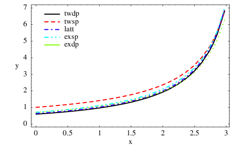
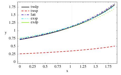
For comparison we also plot results when single pole fit is used. Also in this case we calculate within HMT, take into account both resonances (eq. (5.27a)) and fit the free parameter to the semileptonic decay rate. From the plots it becomes apparent, that our model’s predictions for both and transition form factors are in good agreement with experimental and lattice data when extrapolated with two poles, while single pole extrapolations are not in good agreement with experimental results, especially for transitions indicating that in this extrapolation a single parameter cannot fit both pionic and kaonic decays. This discrepancy further increases if only the first resonance contribution is kept in the calculation for the single pole extrapolation within HMT as was done in previous studies [32]. In such calculations only the resonance contributed, and a lower value of the strong coupling was used. At that time only few decay rates were measured. In comparison with the present experimental data the predicted branching ratios were too large. Note also that the experimental fits on the single pole parametrization of the form factor in transitions done in refs. [117, 118] yielded effective pole masses which are somewhat lower than the physical masses of the meson resonances used in this analysis. The approach of ref. [50] was developed to treat meson semileptonic decay within heavy light meson symmetries in the allowed kinematic region by using the full propagators. We find that this approach cannot reproduce the observed shape of the form factors .
We also compare our predictions for the scalar form factor dependence for the and transitions with those of a successful quark model in ref. [128] and with lattice QCD pole fit analysis of ref. [136]. The results are depicted in fig. 5.5 and fig. 5.6.
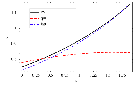
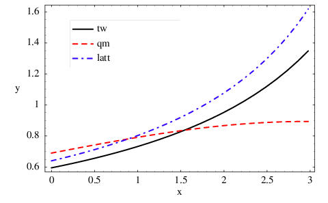
transitions
We next apply the strategy from the previous section to the extrapolation and parameter extraction in transitions. We use the information on the contributions of different resonances to the form factors as suggested by our model. For the vector form factor we thus propose which saturates the effective second pole by the first vector radial excitation . Similarly we set with holding in the exact heavy quark limit, and saturating the poles of the and form factors and the first pole of the form factor with the pseudoscalar radial excitation and the orbital axial excitation respectively. Since our model does not contain a second resonance contribution to the form factor , we impose , effectively sending the second pole mass of this form factor to infinity. At the end we have fixed all the pole parameters appearing in the general form factor parameterization formulas of sec. 5.1.2 using physical information and model predictions on the resonances contributing to the various form factors . The remaining parameters ( and ) are on the other hand related to the parameters of HMT via the model matching conditions at zero recoil.
We again restrict our present study to decays, in order to use the available experimental information in the charm sector, although our calculations can readily be applied to semileptonic decays of mesons once more experimental information becomes available on excited meson resonances. In our numerical analysis we use available experimental information and theoretical predictions on charm meson resonances as in the previous section.
Our HMPT model calculations of section 5.1.3 contain several parameters. The coupling was usually [32, 167] determined from the value of . However, this derivation employed a single pole ansatz for the shape of . One can instead use data on radiative decays. Following discussion in refs. [10, 168], using the most recent data on radiative and strong decays [52], and accounting for the flavor symmetry breaking effects, we calculate GeV-1. The coupling has been estimated in ref. [169] relying on the assumption that the electromagnetic interactions of the light quark within heavy meson are dominated by the exchange of , , vector mesons. We fix the other free parameters () appearing in the HMT Lagrangian and weak currents by comparing our model predictions to known experimental values of branching ratios , , , , as well as partial decay width ratios and [52]. In order to compare the results of our approach with experimental values, we calculate the decay rates for polarized final light vector mesons in eq. (3.35) again with the Wilson coefficient . The constants parametrize the flavor mixing relevant to a particular transition, and are given in table 5.2 together with the pole mesons.
| , | , | ||||
| , | , | ||||
| , | , | ||||
| , | , | ||||
| , | , | ||||
| , | , | ||||
| , | , |
The form factor does not contribute to any decay rate in this approximation and we can not fix the parameters and solely from comparison with experiment. Although actually does contribute indirectly through the relation (3.32) at , this constraint is not automatically satisfied by our model. On the other hand, we can still enforce it ”by hand” after the extrapolation to to obtain some information on these parameters. Due to the specific combinations in which the parameters appear in eqs. (5.35b-5.35g) we are further restrained to determining only the products , and using this kind of analysis. Lastly, since the only relevant contribution of is to the form factor , we cannot disentangle it from the influence of . Yet again we can impose the large energy limit relation (5.16) to extract both values independently.
We calculate the result for , , and by a weighted average of values obtained from all the measured decay rates and their ratios taking into account for the experimental uncertainties. Furthermore, the values of and are extracted separately by minimizing the fit function . Both minimizations are performed in parallel and the global minimum is sought on the hypercube of dimensions in the hyperspace of the fitted parameters. At the end we obtain the following values of parameters:
| (5.37) |
These values qualitatively agree with the analysis done in ref. [32] using a combination of quark model predictions and single pole experimental fits for all the form factors .
We next use these values in relation (3.32) to extract information on the the parameters and . From eqs. (5.35b-5.35g) it is easy to see that the solutions lie on a straight line in the plane. We draw these for the various decay channels used in our analysis in fig. 5.7.

We can see that all the decay channels considered fit approximately the same solution in the plane. Consequently, we can use any point on the approximate solution line to obtain the same prediction for the dependence of the form factor .
It is important to note at this point that due to a high degree of interplay of the various HMT parameters in the model predictions used in the fit, the values of the new model parameters obtained in such a way are very volatile to changes in the other inputs to the fit. Furthermore these are tree level leading order parameter values and may in addition be very sensitive to chiral and corrections. Therefore their stated values should be taken cum grano salis. However more importantly, the form factor , branching ratio and polarization width ratio predictions based on this approach are more robust since they are insensitive to particular combinations of parameter values used, as long as they fit the experimental data. We estimate that chiral and heavy quark symmetry breaking corrections could still modify these predictions by as much as .
We are now ready to draw the dependence of all the form factors for the , and transitions. The results are depicted in figs. 5.8, 5.9, and 5.10.
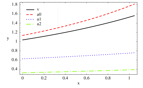
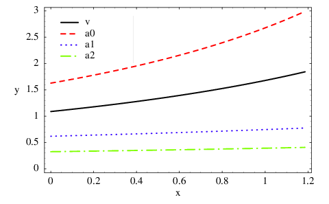
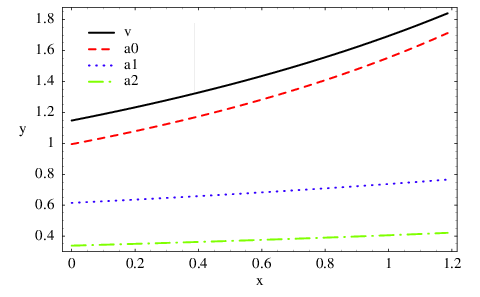
We also compare our model predictions with recent experimental analysis of helicity amplitudes performed by the FOCUS collaboration. Because of the arbitrary normalization of the form factors in [51], we fit our model predictions for a common overall scale in order to compare the results. We plot the dependence of the predicted helicity amplitudes and compare them with the experimental results of FOCUS, scaled by an overall factor determined by the least square fit of our model predictions, in figures 5.11, 5.12 and 5.13. The scale factor is common to all form factors.
In addition to the two pole contributions we calculate helicity amplitudes in the case when all the form factors exhibit single pole behavior. Putting contributions of higher charm resonances to zero, we fit the remaining model parameters to existing branching ratios and partial decay width ratios. We obtain the values for the following parameter combinations:
| (5.38) |
As shown in figures. 5.11 and 5.12 the experimental data for do not favor such a parametrization, while in the case of helicity amplitude there is almost no difference since the helicity amplitude is defined via the form factors , which are in our approach both effectively dominated by a single pole. The agreement between the FOCUS results and our model predictions for the dependence of the helicity amplitudes is good, although as noted already in [51], the uncertainties of the data points are still rather large. In figures. 5.14 and 5.15 we present helicity amplitudes for the and decays. Both decay modes are most promissing for the future experimental studies. We make predictions for the shapes of helicity amplitudes for both cases: where two poles contribute to the vector form factor and a single pole to the axial form factors, and the second case where all form factors exhibit single pole behavior.


5.1.5 Summary
Our predictions for the shapes of the various form factors can also be summarized using the general formulas
| (5.39) |
where as before and . These expressions are actually simplifications of the form factor parameterizations (5.15), (5.18), (5.17) and (5.19) respectively. The parameters , , , , , , , and , which we fix by nearest resonance saturation approximation and HMT calculation at , are listed in tables 5.3 and 5.4 for the various decay channels considered.
| Decay | ||||
|---|---|---|---|---|
| Decay | ||||||
|---|---|---|---|---|---|---|
Finally, using numerical values as explained above, we calculate the branching ratios for all the relevant and semileptonic decays and compare the predictions of our model with experimental data from PDG [52]. The results are summarized in tables 5.5 and 5.6.
| Decay | |||
|---|---|---|---|
| Decay | [%] | (Exp.) [%] | (Exp.) | (Exp.) | ||
|---|---|---|---|---|---|---|
| [53]33 3 Values used in the fit of our model parameters. | ||||||
| [52]33 3 Values used in the fit of our model parameters. | ||||||
| [52]33 3 Values used in the fit of our model parameters. | ||||||
| [52]33 3 Values used in the fit of our model parameters. | [52]33 3 Values used in the fit of our model parameters. | [52]33 3 Values used in the fit of our model parameters. | ||||
| [52]33 3 Values used in the fit of our model parameters. | ||||||
| [53] | ||||||
For comparison we also include in table 5.5 the results for the rates obtained with our approach for (eq. 5.27a) but using a single pole fit. It is very interesting that our model extrapolated with two poles gives branching ratios for in rather good agreement with experimental results for the already measured (partial) decay rates. It is also obvious that the single pole fit gives rates largely incompatible with the experimental results.
We expect as well as chiral corrections in the case of and might further improve the agreement with the experimental data, but due to the presence of a large number of new couplings it is impossible to include them into the calculation within present framework. We expect that the errors in the predicted decays rates stemming from the uncertainties in the input parameters we used can be . In addition, the semileptonic decay rates in our model fit are numerically dominated by the longitudinal helicity amplitude which has a broad pole 44 4 Naive HQET scaling predicts that the helicity amplitude, which scales as should dominate the decay rate.. This is true especially for but to minor extent also for transitions. Since our model parameters are determined at , this gives a poor handle on the dominating effects in the overall decay rate. Thus, accurate determination of the magnitude and shape of the helicity amplitude near would contribute much to clarifying this issue.
In principle one can apply the above procedure to the decays. However, due to the much broader leptons invariant mass dependence in this case, our procedure is much more sensitive to the values of the form factors at and additional contributions beyond the nearest resonances considered here.
To summarize, we have devised a general parametrization of all the and by saturating the form factor dispersion relations with effective poles and encompassing relevant symmetry relations. We conclude that in order to satisfy all the constraints and to be compatible with the available experimental data, one needs at least 1-2 resonant excitations contributing and saturating the form factors’ shapes in the entire physical -region. Our results show, that a single pole parametrization of all the form factors cannot be considered meaningful. Quantitatively, though, we cannot give reliable predictions about the form factors. Our model approach of saturating the effective form factor poles with experimentally measured charmed meson resonances is to be considered as an illustration of the general principles behind the form factor parameterizations.
5.2 Heavy to heavy transitions
In our quest for the precise determination of the CKM matrix element the studies of meson decays into charm resonances have been playing a prominent role. In experiments aimed to determine , actually the product is extracted, where is the or hadronic form factor at zero recoil. A lack of precise information about the shapes of various form factors is thus still the main source of uncertainties. In theoretical studies, heavy quark symmetry has been particularly appealling due to the reduction of six form factors in the case of transitions to only one [170, 171]. In addition, at zero recoil, when the final state meson is at rest in the rest frame, the normalization of the form factors is fixed by symmetry. However, the results obtained within heavy meson effective theories obtain important corrections coming from operators which are suppressed as [172] as well as of higher order in the chiral expansion [32, 54, 173, 174]. The knowledge of both kinds of corrections has improved during the last few years. The decay amplitude is corrected by only at the second order in this expansion making it more appropriate for the experimental studies [32, 175]. In addition to heavy meson effective theory, other approaches have been used in the study of the form factors, such as quark models [176] and QCD sum rules [177], while the most reliable results should be expected from lattice QCD [178]. In the treatment of hadronic properties using lattice QCD the main problems arise due to the small masses of the light quarks. Namely, lattice studies have to consider light quarks with larger masses and then extrapolate results to their physical values. In these studies the chiral behavior of the amplitudes is particularly important. HMPT is very useful in giving us some control over the uncertainties appearing when the chiral limit is approached. Most recently in ref. [179], the authors have discussed and form factors in staggered PT by including the chiral loop corrections.
In this section we investigate chiral loop corrections within HMPT in the semileptonic transitions of mesons into charm mesons of positive and negative parities to determine their impact on the chiral extrapolation used by lattice QCD studies of the relevant form factors.
5.2.1 form factors
The weak vector current matrix element between heavy and mesons with velocities and respectively can be parametrized in terms of two velocity dependent form factors [33]
| (5.40) |
where and with similar formulae for the vector and axial current matrix elements between and the vector or scalar charmed states. The differential decay rate in terms of these form factors is
| (5.41) |
where and we have assumed the form factor is real throughout the kinematically allowed region . It can be related to via
| (5.42) |
Again similar formulae are valid for and transitions.
5.2.2 Framework and Calculation of Chiral Loop Corrections
We use the formalism of heavy meson chiral Lagrangians of the previous sections. The weak part of the Lagrangian describing transitions among heavy quarks can be matched upon weak heavy quark currents in HQET [54, 55]
| (5.43) | |||||
at leading order in chiral and heavy quark expansion and where . Evaluating the traces in the first term on the r.h.s we can identify for example
| (5.44) |
resulting in the HQET predictions and . Note that heavy quark symmetry dictates the values of , which should not receive any chiral corrections. On the other hand is not constrained and we use the recently determined value of [180] .
We first calculate the wave function renormalization of the heavy and , fields. This has been done in the chapter 4. We get non-zero contributions to the heavy meson wavefunction renormalization from the self energy (”sunrise” topology) diagrams in fig. 4.1 with leading order couplings in the loop . In the case of the mesons both vector and scalar mesons can contribute in the loop. The positive parity and similarly obtain wavefunction renormalization contributions from self energy diagrams (fig. 4.1) with , and , , mesons in the loops respectively. Then we calculate loop corrections to the Isgur -Wise functions , and . These come from the diagram topologies as the one shown fig. (5.16).
Namely the initial and final heavy states may exchange a pseudo-Goldstone, while pairs of positive and negative parity heavy mesons may propagate in the loop. Again not all heavy states contribute due to parity conservation in effective strong interaction vertices. Thus, when initial and final states are pseudoscalars we get contributions from pairs of , , and propagating in the loop, while for pseudoscalar initial and scalar final state we get contributions from pairs of , , and in the loop (due to heavy quark symmetry, the same results are obtained for (axial)vector external states, although different intermediate states contribute). The complete expressions for the loop corrected , and we obtain, are listed below. For the we get
where the same formulae can be applied to with the substitution and . For the on the other hand we obtain
In the above expressions are the chiral loop corrections to the heavy meson wavefunction renormalization for the negative and positive parity doublets is given in eqs. (4.3) and (4.4). As in ref. [43] and in previous sections, a trace is assumed over the inner repeated index(es) (here ), while the complete expressions for the loop integral functions can be found in Appendix B.
5.2.3 Chiral Extrapolation
We study the contributions of the additional resonances in the chiral loops to the chiral extrapolations employed by lattice QCD studies to run the light meson masses from the large values used in the simulations to the chiral limit [45, 46]. In order to tame the chiral behavior of the amplites containing the mass gap between the ground state and excited heavy meson states we again use the expansion of the chiral loop integrals from section 4.4.1 so that we obtain for the non-analytic terms
| (5.47) | |||||
and
where
| (5.49) |
so that and . The first lines of eqs. (5.47) and () contain the leading contributions while the calculated corrections are contained in the second lines. Note that the positive parity heavy mesons contribute only at the order in this expansion since all the possible contributions vanish in dimensional regularization and the affected loop integral expressions have to be expanded up to the second order in .
As argued in section 4.4.1 the expansion works well in an theory where kaons and etas, whose masses would compete with the splitting, do not propagate in the loops. Therefore we write down explicit expressions for the chiral loop corrected Isgur-Wise functions specifically for the strangeless states () in the theory:
| (5.50) | |||||
and
We then plot the chiral behavior of the Isgur-Wise function renormalization in the chiral limit below the scale in figs. 5.17 and 5.18.
We again normalize the values of the extrapolated quantities at to and perform the chiral extrapolation using the Gell-Mann formulae (eq. (2.6)). Presently no reliable estimates exist for the values of and , which feature in chiral extrapolation involving opposite parity heavy states. Therefore we estimate their possible effects by varying their relative values in respect to between and in our extrapolations. We see that the effects of positive parity states’ in the chiral loops on the chiral extrapolation of appear to be mild (around one percent in our estimate) below the scale (the gray shaded region around the leading order result in black solid line). Actually if is positive as reasoned in [54] and around , these leading corrections almost vanish. The same general chiral behavior can be attributed to with the substitutions , and . Also, the chiral extrapolation (including small leading contributions) of the normalization appears fairly flat, indicating a linear extrapolation as a good approximation, whereas the effects of chiral loops on the extrapolation of its slope appear to be sizable, up to in our crude estimate.
5.3 Discussion and Conclusion
In this chapter we have calculated chiral loop corrections to and functions within a HMPT framework, which includes even and odd parity heavy meson interactions with light pseudoscalars as pseudo-Goldstone bosons. Our analysis confirms that the form of the leading pionic logarithmic corrections to the Isgur-Wise functions is not changed by the inclusion opposite parity heavy mesons; they only contribute at the order as can be inferred by comparing Eq. (5.47) with Eq. (8) of Ref. [174].
These results are particularly important for the lattice QCD extraction of the form factors. The present errors on the parameters in the exclusive channels are of the order few percent. This calls for careful control over theoretical uncertainties in its extraction. The understanding of chiral corrections is crucial in assuring validity of the form factor extraction and error estimation coming from the lattice. Our estimates for the leading corrections also constrain the accuracy of such extrapolations. From these results one can deduce also the chiral corrections in the decays which are not approached by experiment. Due to the strange quark flavor of final and intital heavy meson states, there is no leading pion logarithmic corrections making the lattice extraction below the heavy meson parity splitting gap much simpler.
In the expansion the opposite parity contributions yield formally next-to-leading chiral log order corrections in a theory with dynamical heavy meson fields of only single parity. Therefore they compete with corrections due to counterterm operators of higher chiral powers within chiral loops (see e.g. fig. 5.19), where is the chiral symmetry breaking cut-off scale of the effective theory.
In a theory containing propagating heavy meson states of both parities, the inclusion of such terms would in addition also yield terms. Our present approach to the estimation of the positive parity effects on the chiral extrapolation is therefore valid with the assumption where these additional contributions are further suppressed.
Chapter 6 Heavy neutral meson mixing
The oscillations in the systems are mediated by FCNCs which are forbidden at tree level of the SM and therefore their detection gives access to the particle content in the corresponding loop diagrams. First experimental measurement of a large value of indicated that the top quark mass was very heavy [181], which was confirmed almost a decade later in the direct measurements through the -collisions, [182]. Nowadays, the accurately measured [56], and [57], are used to constrain the shape of the CKM unitarity triangle and thereby determine the amount of the CP-violation in SM [4, 3]. This goal is somewhat hampered by the theoretical uncertainties in computing the values for the two decay constants, , and the corresponding “bag” parameters, . These quantities can, in principle, be computed on the lattice. 11 1 Recent reviews on the current status of the lattice QCD computations of mixing amplitudes can be found in ref. [183, 184, 185, 186]. However, a major obstacle in the current lattice studies is that the -quark cannot be reached directly but through an extrapolation of the results obtained by working with larger light quark masses down to the physical -quark mass. In this chapter we investigate the effects of including positive parity heavy mesons into chiral extrapolation calculations on the specific examples of the decay constants and the bag parameters which enter the investigation of the SM and SUSY effects in the and mixing amplitudes [187, 188, 189, 190, 191].
6.1 operator basis and mixing
The SUSY contributions to the mixing amplitude, where stands for either - or -quark, are usually discussed in the so called SUSY basis of operators [58]:
| (6.1) | |||||
where and are the color indices. Although the operators in the above bases are written with both parity even and parity odd parts, only the parity even ones survive in the matrix elements. In SM, only (left–left) operator is relevant in describing the mixing amplitude. The matrix elements of the above operators are conventionally parameterized in terms of bag parameters, , as a measure of the discrepancy with respect to the estimate obtained by using the VSA,
| (6.2) |
where is the renormalization scale of the logarithmically divergent operators, , at which the separation between the long-distance (matrix elements) and short-distance (Wilson coefficients) physics is made. Explicit calculation yields
| (6.3a) | |||||
| (6.3b) | |||||
| (6.3c) | |||||
| (6.3d) | |||||
| (6.3e) | |||||
with and being the axial current and the pseudoscalar density, respectively. Next we switch to HQET, by replacing the the field with the static one introduced in section 2.3 – , satisfying . This equation and the fact that that the amplitude is invariant under the Fierz transformation in Dirac indices, eliminate the operator from further discussion, i.e., , where the tilde is used to stress that the operators are now being considered in the static limit of HQET (). Furthermore, in the same limit
| (6.4) |
where is the decay constant of the static heavy-light meson, and the HQET states are normalized as , so that we finally have
| (6.5a) | |||||
| (6.5b) | |||||
| (6.5c) | |||||
| (6.5d) | |||||
One of the reasons why lattice QCD is the best currently available method for computing these matrix elements is the fact that it enables a control over the -dependence by verifying the corresponding renormalization group equations, which is essential for the cancellation against the -dependence in the corresponding perturbatively computed Wilson coefficients [192, 193, 194]. From now on we will assume that the UV divergences are being taken care of and the scale will be implicit.
6.2 Chiral logarithmic corrections
In this section we use HMPT to describe the low energy behavior of the matrix elements (6.5a-6.5d). Before entering the details, we notice that the operators and differ only in the color indices, i.e., by a gluon exchange, which is a local effect that cannot influence the long distance behavior described by PT. In other words, from the point of view of PT, the entire difference of the chiral behavior of the bag parameters and is encoded in the local counterterms, whereas their chiral logarithmic behavior is the same. Similar observation has been made for the operators entering the SUSY analysis of the - mixing amplitude, as well as for the electromagnetic penguin operators in decay [59]. Thus, in the static heavy quark limit (), we are left with the first three operators (6.5a-6.5c) which, in their bosonized version, can be written as [195]
| (6.6a) | |||||
| (6.6b) | |||||
| (6.6c) | |||||
where 22 2 Contraction of Lorentz indices and HQET parity conservation requires the same to appear in both traces of a summation term. Any insertions of can be absorbed via , while any non-factorisable contribution with a single trace over Dirac matrices can be reduced to this form by using the matrix identity . As before the index “” denotes the light quark flavor, and ‘‘c.t.” stands for the local counterterms. To relate ’s to the bag parameters in eq. (6.5a-6.5d) we evaluate the traces in eq. (6.6a-6.6c) to obtain33 3 Our convention differs by a factor of two, compared to those of [195]. This is due to our use of combined positive and negative frequency fields which yield this additional factor in mixed terms which always appear twice.
| (6.7) |
where
| (6.8a) | |||||
| (6.8b) | |||||
| (6.8c) | |||||
We will use the known form of the HMPT Lagrangian (2.19). To get the chiral logarithmic corrections to -parameters, we should subtract twice the chiral corrections to the decay constant from the chiral corrections to the four-quark operators (6.6a-6.6c). The former is obtained from the study of the bosonized left-handed weak current (2.20) for the negative parity heavy mesons. Here we shall also consider the next-to-leading order chiral counterterm contributions and we write it as
| (6.9) |
where is the tree level decay constant in the chiral expansion, and are the counterterm coefficients. Together with the strong coupling , these parameters are not predicted within HMPT. Instead, they are expected to be fixed by matching the HMPT expressions with the results of lattice QCD for a given quantity (see reviews in ref. [196, 197, 198]). The notation used above is the same as in ref. [153].
The chiral logarithmic corrections to the decay constant come from the diagrams shown in fig. 6.1
| (6.10) |
where it should be stressed that we work in the exact isospin limit () so that the index means either - or -quark. Only explicit in the above expressions is the term arising from the tadpole diagram (in fig. 6.1), whereas , the heavy meson field renormalization factors, come from the self energy diagram (left in fig. 6.1) and are given in eq. (4.3). We write out the leading order contributions of negative parity heavy states only
In both eqs. (6.2) and (6.2) the dependence in the logarithm cancels against the one in the local counterterms.
With these ingredients in hands it is now easy to deduce that the only diagrams which contribute to the SM bag parameter, , are the two shown in fig. 6.2. They arise from the two terms in and yield
| (6.12a) | |||||
| (6.12b) | |||||
respectively, where are the SU(3) generators and masses of the pseudo-Goldstone bosons. The SM bag parameters now read
| (6.13) |
where we also wrote the counterterm contributions and, for short, we wrote . The above results agree with the ones presented in refs. [199, 200], in which the pion loop contribution was left out, and with the ones recently presented in ref. [201].
6.3 Impact of the -mesons
In this section we examine the impact of the heavy-light mesons belonging to the doublet when propagating in the loops onto the chiral logarithmic corrections derived in the previous section. We use the full Lagrangian of eq. (2.19) and also the weak current operators (2.20), which we also extend for the heavy meson chiral counterterm contributions:
| (6.15) |
where are the coefficients of two new counterterms.
6.3.1 Decay constants
Since we focus on the pseudoscalar meson decay constant, it should be clear that only the scalar meson from the doublet can propagate in the loop . The diagrams that give non-vanishing contributions are shown in fig. 6.3 and the corresponding expressions now read
| (6.16) | |||||
where the summation over “” is implicit, and we omit the counterterm contributions to make the expressions simpler. The integral functions can be found in Appendix B. The last term in the decay constant (the one proportional to ) comes from the right graph in fig. 6.3 which was absent before the inclusion of the scalar meson. Notice that due to the chiral behavior of the functions in eq. (4.13), the presence of the nearby state does not affect the pionic logarithmic behavior of the decay constant. It does, however, affect the kaon and -meson loops because those states are heavier than and the coefficients of their logarithms cease to be the predictions of this approach since those logarithms are competitive in size with the terms proportional to . Stated equivalently, the relevant chiral logarithmic corrections are those coming from the theory, and the pseudoscalar decay constant reads
| (6.17) |
where stands for the combination of the counterterm coefficients considered in the previous section. 44 4 More specifically, , where we use the Gell-Mann–Oakes–Renner formula, from eq. (2.6). We stress again that the exact isospin symmetry ( ) is assumed throughout this chapter. At this point we also note that we checked that the chiral logarithms in the scalar heavy-light meson decay constant, which has recently been computed on the lattice in ref. [165, 46], are the same as for the pseudoscalar meson, with the coupling being replaced by , i.e.,
| (6.18) |
Since, as we already checked in chapter 4 (see table 4.1) the deviation from the linear behavior in is less pronounced for than it is for .
6.3.2 Bag parameters
In this subsection we show that the situation with the bag parameters is similar to the one with decay constant, namely the pion loop chiral logarithms remain unchanged when the nearby scalar meson is included in HMPT. To that end, besides eq. (2.19), we should include the contributions of -mesons to the operators (6.6a-6.6c). Generically the operators now become
| (6.19) | |||||
where are the couplings of the operator to both and mesons, while come from the coupling to the mesons only. Similarly, the operators now read:
| (6.20) | |||||
| (6.21) | |||||
After evaluating the traces in eqs. (6.19), and keeping in mind that the external states are the pseudoscalar mesons, we have
| (6.22) | |||||
where have forms analogous to the ones written in eq. (6.8a).
The corresponding additional 1-loop chiral diagrams are shown in fig. 6.4. Since the couplings of the four-quark operators to the scalar meson(s) are proportional to and of the pseudoscalar decay constant to , the cancellation between the chiral loop corrections in the operators and in the decay constant is not automatic. For that reason, instead of writing the chiral logarithmic corrections to the bag-parameter, we will write them for the full operator, namely
To keep the above expression simpler we do not write the counterterms since their structure remains the same as before. The similar formulae for are
We now turn to the case and study the behavior of eq. (6.3.2) around . We shall proceed similarly to what has been done in section 4.4.1, namely we expand the integrand in . We see that after expanding eq. (6.3.2) around , the leading chiral logarithms arising from the pion loops remain unchanged even when the coupling to the scalar meson is included in the loops. On the other hand, as discussed in the previous subsection, the logarithms arising from the kaon and the -meson are competitive in size with those arising from the coupling to the heavy-light scalar meson, which is the consequence of the smallness of . Therefore, like for the decay constants, the relevant chiral expansion is the one derived in the theory, i.e.,
| (6.26a) | |||||
| (6.26b) | |||||
or by using eq. (6.17), for the bag parameters we obtain
| (6.27a) | |||||
| (6.27b) | |||||
which coincide with the pion loop contributions shown in eqs. (6.2) and (6.2), as they should.
6.4 Relevance to the analysis of the lattice QCD data
It should be stressed that the consequence of the discussion in the previous section is mainly important to the phenomenological approaches in which the sizable kaon and -meson logarithmic corrections are taken as predictions, whereas the counterterm coefficients are fixed by matching to large expansion or some other model. We showed that the contributions of the nearby heavy-light scalar states are competitive in size and thus they cannot be ignored nor separated from the discussion of the kaon and/or -meson loops. However, the fact that the nearby scalar heavy-light mesons do not spoil the dominant pion logarithmic correction to the decay constant and the bag-parameters is most welcome from the lattice practitioners’ point of view, because the formulae derived in HMPT can still (and should) be used to guide the chiral extrapolations of the lattice results, albeit for the pion masses lighter than .
6.5 Conclusion
In this chapter we revisited the computation of the mixing amplitudes in the framework of HMPT. Besides the SM bag parameter, we also provided the expressions for the chiral logarithmic correction to the SUSY bag parameters. More importantly, we study the impact of the near scalar mesons to the predictions derived in HMPT in which these contributions were previously ignored. We showed that while the corrections due to the nearness of the scalar mesons are competitive in size with the kaon and meson loop corrections, they do not alter the pion chiral logarithms. In other words the valid (pertinent) PT expressions for the quantities discussed in this chapter are those involving pions only. This is of major importance for the chiral extrapolations of the results obtained from the QCD simulations on the lattice, because precisely the pion chiral logarithms provide the most important guideline in those extrapolations. As a side-result we verified that the chiral logarithmic corrections to the scalar meson decay constant are the same as to the pseudoscalar one, modulo replacement (c.f. eq. (6.18)).
Chapter 7 and rare hadronic decays of mesons
Rare decays of mesons are considered to be one of the promising areas for the discovery of new physics beyond the SM [60, 61, 62]. This is based on the expectation that virtual new particles will affect these decays, in particular in processes induced by FCNCs; such processes are suppressed in the SM since they proceed via loop diagrams. This venue, typified by transitions like , has been investigated intensively in recent years [60, 61, 62]. In particular the experimental results on decay rates and the parameters describing CP-violation in the meson nonleptonic two-body weak decays such as and have attracted a lot of attention during the last few years (see e.g. [202] and references therein). In the theoretical explanation of these decay rates and CP violating parameters it is usually assumed that an interplay of the SM contributions and new physics occurs. Grossman et al. [69] have investigated the decay mechanisms of decays and found that new physics might give important contributions to the relevant observables. In their search for the explanation of the puzzle, the authors of [203] have investigated the decay mode within a model with an extra flavor changing boson, making predictions for the CP violating asymmetries in these decays . mediated penguin operators have also been considered in many other scenarios. Contributions of SUSY models with and without R-parity violation (RPV) in the same decay channel were also discussed in [204]. The difficulty with this decay mode is that the SM contribution is the dominant one. The use of QCD in the treatment of the weak hadronic meson decays is not a straightforward procedure. Numerous theoretical studies have been attempted to obtain the most appropriate framework to describe nonleptonic meson decays to two light meson states. But even the most sophisticated approaches such as QCD factorization (BBNS and SCET) [148, 205, 206, 207, 208, 209, 210, 211, 212, 213, 214, 215] still have parameters which are difficult to obtain from ‘‘first principles’’. Consequently, searches for new physics in decay modes dominated by SM contributions suffer from large uncertainties.
A related, though alternative approach is the search for rare decays which have extremely small rates in the SM, and their mere detection would be a sign for new physics. Several years ago, Huitu, Lu, Singer and Zhang suggested [63, 64] the study of and as prototypes of the alternative method. This proposal is based [63] on the fact that these transitions are indeed exceedingly small in the SM, where they occur via box diagrams with up-type quarks and ’s in the box. The matrix elements of these transitions are approximately proportional in SM to and ( is the sine of the Cabibbo angle), resulting in branching ratios of approximately and respectively, probably too small for detection even at LHC. Further discussions on these () and () transitions are given in Refs. [69, 216, 217, 218].
Huitu et al. have then investigated [62, 63] the transition in several models of physics beyond SM, namely the MSSM, the MSSM with RPV couplings and the THDM. Within a certain range of allowed parameters, the MSSM predicts [63] a branching ratio as high as for . On the other hand, Higgs models may lead [64] to a branching ratio at the level. Most interestingly, in RPV the process can proceed as a tree diagram [63] and limits on RPV superpotential couplings that existed at the time did not constrain at all the transition.
In Ref. [63] the hadronic decay , proceeding either directly or through a , has been selected as a convenient signal for the transition. A rough estimate [63] has shown that the semi-inclusive decays may account for about of the transitions. The OPAL collaboration has undertaken the search for this decay establishing [219] the first upper limit for it, subsequently constrained by both B-factories [68, 220, 221] to . In an experiment planned [222] by ATLAS at LHC, a two orders of magnitude improvement is expected.
In order to use these results for restricting the size of the and transitions one needs also an estimate for the long distance contributions to such ( and ) processes. A calculation [223] of such contributions provided by and by intermediate states as well as those induced by virtual and mesons lead to a branching ratio , only slightly larger than the short-distance result of SM for this transition. Thus, this decay and similar ones are indeed suitable for the search of new physics, the LD contribution not overshadowing the new physics, if it leads to rates of the order of or larger. A survey [224] of various possible two-body () decays of mesons to , , states has singled out and as the most likely ones for the detection of the presence of RPV transitions at the level.
The transition has not been subject of such intensive theoretical studies although experimental information on the upper bound for the decay rate already exists. Namely, the BaBar collaboration has reported that [221] while the Belle collaboration found [68]. The LHC-b is expected to give even better constraints. Therefore we shall consider possible candidate nonleptonic decay channels proceeding with the transition for the experimental searches.
At the forthcoming LHC accelerator one expects about events/year, at a luminosity of [65]. Even if the actual number will be a couple of orders of magnitude lower, the search for rare decays of exhibiting possible features of physics beyond SM will become possible. The effect of such physics on radiative decays of , as caused for example by -quark decay via the transition has already been investigated [225, 226]. Here, we will address the effects of new physics on rare -decays caused by the ( and ) transitions, which we already mentioned to be very rare in SM [63, 64, 69]. Specifically, we will calculate two-body decay modes , and as well as three body modes , , , , , and . We expect these modes to be most likely candidates for the experimental observation.
7.1 Inclusive and transitions in SM and beyond
7.1.1 Operator basis and mixing
The effective weak Hamiltonian encompassing the process has been introduced by the authors of [69] in the case of decays. Following their notation we also include the transitions and write it as
| (7.1) |
where and denote effective Wilson coefficients multiplying the complete operator basis of all the four quark operators which can contribute to the processes (for ) and (for ). We choose
| (7.2) |
plus additional operators , with the chirality exchanges , plus the same operators with and quark flavors interchanged. In these expressions, the superscripts are color indices. All other operators
with the correct Lorentz and color structure can be related to these by operator identities and Fierz rearrangements. We perform our calculations of inclusive and exclusive decays at the scale of the quark mass (), therefore we have to take into account the RGE running of these operators from the interaction scale . At leading log order in the strong coupling, the operators mix with the anomalous dimension matrix
| (7.3) |
The same holds for operators () due to Fierz identities, while the operator has anomalous dimension . Anomalous dimension matrices for chirally flipped operators are identical to these.
7.1.2 SM
Within the SM only the operators contribute to the () transitions at one loop. The dominating contributions to the Wilson coefficients come from the up quark and boson box diagrams in fig. 7.1.
The top and charm quark loop contributions dominate and lead to
| (7.4a) | |||||
| (7.4b) | |||||
where
| (7.5a) | |||||
| (7.5b) | |||||
Using numerical values of the relevant CKM matrix elements from PDG [52] and possibly including the CKM phase in one always finds and . Renormalization group running from the weak interaction scale to the bottom quark mass scale, due to anomalous dimension of the operator , induces only a small correction factor of which can be safely neglected. The inclusive amd decay widths within SM can then be calculated. By accounting for the colors of final state quarks in combination with the crossing symmetry one obtains
| (7.6) |
which leads to the branching ratios of the order (for ) to (for ).
7.1.3 Beyond SM
Next we discuss contributions of several models containing physics beyond the SM : the MSSM with and without RPV and models with an extra boson. For the THDM on the other hand, the charged Higgs box diagram contributions were found to be negligible in the case [64]. Due to higher CKM suppression, the argument holds also for the case. In addition, the tree level neutral Higgs exchange amplitude for is proportional to , where and are flavor changing Yukawa couplings and is a common Higgs mass scale. This ratio is constrained from the neutral meson mixing [64]. Using presently known values of and [52] one can obtain an upper bound of rendering this contribution negligible. Similarly for the process the relevant effective THDM coupling is bounded from above by the upper limit on . With the recent two-sided bound on the oscillation frequency from the D0 and CDF collaborations [57, 79] it is now possible to constrain this contribution to . This value is two orders of magnitude smaller than the one used in existing studies. Correspondingly, all the decay rate predictions for the THDM are diminished by four orders of magnitude and thus rendered negligible.
MSSM
In the MSSM, like in the SM , the main contributions come from the operators , while the corresponding Wilson coefficients are here
| (7.7a) | |||||
| (7.7b) | |||||
as found in analyses [58] taking into account only contributions from the left-handed squarks in the loop (see fig. 7.2).
Recently it has been also verified [218] that the chargino contribution in MSSM to this process is indeed smaller by an order of magnitude than contributions calculated in [63]. The functions and read [58]
| (7.8a) | |||
| (7.8b) | |||
with . We take [52], while couplings parametrize the mixing between the down-type left-handed squarks. The value of is determined from the mixing [58] and is currently bounded by [52]. We follow ref. [227] and take ; using results from [58] we estimate the absolute value of to be below at average squark mass . The strongest bounds on come from the radiative decay [58, 228, 229]. These studies give at and for the stronger bound on which results in . This updated value for is somewhat smaller than those used in [63, 224]. Similarly, the recent limits on [227, 230, 231] disallow significant contributions from the mixed and the right-handed squark mass insertion terms. Therefore, we only include the dominant contributions given in the above expression. We follow ref. [227] and take and the corresponding values of and [58]. We take for the average mass of squarks , and find . Using expression (7.6) and substituting for the correct Wilson coefficient one finds the MSSM prediction for the inclusive and decay branching ratios of the order of .
RPV
If RPV interactions are included in the MSSM, the part of the superpotential which becomes relevant here is , where and are family indices, and , and are superfields for the lepton doublet, the quark doublet, and the down-type quark singlet, respectively.
The tree level effective Hamiltonian due to sneutrino exchanges in fig. 7.3 receives contributions from the operators and with the Wilson coefficients defined at the interaction scale
The QCD corrections were found to be important for this transition [232]. For our purpose it suffices to follow [63] retaining the leading order QCD result. Namely, the RGE running of the operators induces a common correction factor for and :
| (7.10) |
which evaluates to for a range of sneutrino masses between . In addition the mixing with the operators and induces a small contribution to the Wilson coefficients and :
| (7.11) |
which is of the order for the chosen sneutrino mass range. The relevant part of the effective Hamiltonian we use in this scenario is then
| (7.12) | |||||
We neglect the suppressed contributions of , to the amplitudes in the cases where the operators , give non-zero contribution. The inclusive and decay rates induced by the RPV model become
| (7.13) |
Z’
In many extensions of the SM [66] an additional neutral gauge boson appears. Heavy neutral bosons are also present in many extensions of the SM such as grand unified, superstring theories and theories with large extra dimensions [67]. This induces contributions in fig. 7.4 to the effective tree level Hamiltonian from the operators as well as .
Following [66, 67], the Wilson coefficients for the corresponding operators read at the interaction scale
| (7.14) |
where and . In this expression , , and stand for the gauge couplings and masses of the and bosons, respectively, while is their mixing angle. Again renormalization group running induces corrections and mixing between the operators. As already mentioned, the mixing of operators and their chirally flipped counterparts is identical to that of operators since these operators are connected via Fierz rearrangement. Thus the same scaling and mixing factors and apply. For the operator on the other hand the renormalization can be written as with
| (7.15) |
In particular for a common boson scale of [66] one gets numerically , and . The full contributing part of the effective Hamiltonian in this case is
| (7.16) | |||||
For the inclusive and decay rates the and are numerically suppressed due to the factor and we write
| (7.17) |
In Section 7.3 we discuss bounds on Wilson coefficients and which might be estimated from the and decay rates.
7.2 Two- and three-body non-leptonic decays of mesons
In calculating decay rates of various meson decay modes based on the and quark transition, one has to calculate matrix elements of the effective Hamiltonian operators between meson states. As a first approximation, the calculation will be performed in the factorization approximation. In the meson decays this works in a good number of cases, while in other cases a more sophisticated approach is needed (for a recent review see [233]). In this first calculation we consider that factorization approximation is sufficient for obtaining the correct features of the decays of the various channels considered. An exception is the case in which matrix elements vanish as a result of factorization, which in a better approximation can be improved.
7.2.1 Preliminaries
In out naïve factorization of two- and three-body amplitudes, we express the resulting one- and two-point transition amplitudes between mesons in terms of the standard weak transition decay constants and form factors (3.20a - 3.21), as dictated by the Lorentz covariance. Some general formulae can be devised to assist our calculation.
Factorization and Kinematics
For the decays of a pseudoscalar meson containing a quark to two mesons and two diagram topologies are possible in the factorization approximation (in fig. 7.5). The right “anhilation” diagram does not contribute in spectator processes, where the light quark flavor of the meson ( in and in ) does not feature in the effective Hamiltonian. All processes that we shall consider are of this type.
We first derive a general expression for the factorized matrix element of the operators , relevant in the framework of SM (MSSM). In case the final state mesons are pseudoscalars (we deonte them by and ) we get for the
| (7.18) |
Taking care of sign difference due to different chirality structure, the same expression also applies for operators , and .
Similarly, when one of the final state mesons is a vector (we denote it as ), we have two possibilities: either (I) the vector state is paired with the vacuum or (II) with the initial meson. The two possibilities give
| (7.19a) | |||||
| (7.19b) | |||||
Because only vector currents contribute in the expression (I), it also applies for operators , and , while in the case (II) the expression is valid for these operators up to a sign difference.
In two-body decays with a vector meson and a pseudoscalar meson in the final state we also sum over the polarizations of . The sum in our case reduces to
| (7.20) |
where is the polarization vector of and is defined as .
For decay to two vector mesons in the final state we use the helicity amplitudes formalism as described in ref. [234]. Non-polarized decay rate is expressed as an incoherent sum of helicity amplitudes
| (7.21) |
where is momentum of the vector meson in meson rest frame and helicity amplitudes are expressed as
| (7.22) |
Vector meson masses are denoted by , while definition of the constants , and is given by general Lorentz decomposition of the polarized amplitude
| (7.23) |
where and are the vector mesons polarizations and momenta.
Situation is more complicated in the case of three body nonleptonic decays. Beside the simple factorized topology in the center of figure 7.6, we also need to consider possible dominant contributions comming from (resonant) intermediate states, such as those pictured in the left and right diagrams in fig. 7.6.
Here again the left diagram does not contribute in our chosen “spectator” channels. For the decays of to three pseudoscalar mesons , and the factorized matrix element of due to the topology in center fig. 7.6 reads
| (7.24) |
Because only vector currents contribute in the above expression, it also applies for operators , and . The Mandelstam kinematical variables are as before , and . We assume these contributions to be the dominant ones, where present. Possible contributions from the right diagram of fig. 7.6 are to be considered where eq. (7.24) does not contribute. We employ resonance dominance approximation and saturate the intermediate state with the lowest lying resonances coupling to the weak current and the pair of final state mesons. The lowest resonance coupling to a pair of pseudoscalar mesons in a parity conserving way is of vector type (we denote it as ) and only contributes via the (pseudo)scalar part of the current. Therefore we may write such contribution as
| (7.25) |
where is the meson propagator of Breit-Wigner form, while is the strong transition matrix element defined in eq. (3.19) and needs to be calculated in a suitable QCD effective theory description or model. Contraction of propagator Lorentz indices with vector state polarizations is understood. The amplitude thus becomes
| (7.26) |
Other possible three-body decay channels with vector mesons in final states will not be considered as they are very difficult to reconstruct experimentaly.
In the context of RPV, the contributions of the operators and to hadronic amplitudes are dominant. One can use the Dirac equation to express scalar (pseudoscalar) density operators in terms of derivatives of vector (axial-vector) currents
| (7.27) |
Using these relations we can derive expressions for the factorized matrix element of the and operators in all two- and threebody channels considered above. For the two-body case we obtain
| (7.28) |
In channels, only case (II) (eq. (7.19b)) contributes in the factorization approximation due to the vector polarization transverzality condition in case (I). This gives
| (7.29) |
Vector transversality condition also kills any and contributions in channels. For the three-body channel topology in fig. 7.6 on the other hand one obtains
| (7.30) |
and for the resonance contribution (fig. 7.6)
| (7.31) |
Finally, the color non-singlet operators and can be Fierz rearranged to and and then same expressions apply as well. Remaining operators are all of the form and their forms are therefore given above.
Modeling Form Factors
In our calculations we need the transition form factors , and . Since HQET and the whole discussion of chapter 5 is not directly applicable to the decays of the meson, we assume pole dominance for these form factors [93, 235]:
| (7.32) |
and take numerical values for and from from QCD sum rules calculations [235] (see tables 7.1 and 7.2).
| Decays | ||||||
|---|---|---|---|---|---|---|
| Decays | ||||||
|---|---|---|---|---|---|---|
For the and transitions used to constrain new physics model parameters we use the form factors calculated in the relativistic constituent quark model with numerical input from lattice QCD at high [128]
| (7.33a) | ||||
| (7.33b) | ||||
| (7.33c) | ||||
| (7.33d) | ||||
In the three body decay modes involving pairs of and mesons, we also need the form factors for the transitions. These are not available in the literature and we calculate them by utilizing HMPT, including the light scalar meson interactions with heavy mesons as it has been done recently [95], and presuming the main contributions from exchange of light scalar meson resonance . Interactions of heavy mesons are described by the HMPT Lagrangian 2.19, to which we add interactions of scalar mesons, which we put into an nonet () representation
| (7.34) |
Here the light scalar mesons are introduced through the field, where is the light scalar meson matrix
| (7.35) |
The ellipses indicate further terms involving only light meson fields, chiral and corrections. At the leading order in heavy quark mass and chiral expansion , is found to vanish, so the only contributions come from the form factor . We then use resonance dominance appoximation to obtain
| (7.36) |
From our analyses in Chapter 5 this result comes as no suprise since our choice of form factor parameterization dictates which resonances may contribute. Taking account of only (pseudo)scalar resonance exchange thus singles out the form factor . In the numerical calculation we use [95]. The rest of parameters are taken from PDG [52].
7.2.2 Amplitudes
and
Experimentally, these are the only constrained processes proceeding through the and transitions. Therefore we may constrain new physics model parameters and use these constraints to predict other viable decay channels .
Hadronic matrix element entering in the amplitudes for () in SM (MSSM) is readily given by eq. (7.24) after identifying , , and using appropriate form factors . Eq. (7.30) is used instead for RPV, while the amplitude incorporates both eqs. (7.24) and (7.30). There are two contributions in each model to this mode, with an additional term with the () replacement in eqs. (7.24) and (7.30), representing an interchange of the two pions (kaons) in the final state. After phase space integration, the decay rates can be written very compactly with only Wilson coefficients left in symbolic form in table 7.3.
| Model | ||
|---|---|---|
| (MS)SM | ||
| RPV | ||
| Z’ | ||
and
In calculation of the () decay rates again we use eqs. (7.24) and (7.30) now with substitutions , and . Numerical results are presented in table 7.4.
| Model | ||
|---|---|---|
| (MS)SM | ||
| RPV | ||
| Z’ | ||
These decay rates are suppressed due to the small phase space in comparison to the rates of the and decays. In numerical analysis we will again and in all following cases neglect all the interference terms appearing in RPV and models.
and
Here we identify , and and obtain results in table 7.5.
| Model | ||
|---|---|---|
| (MS)SM | ||
| RPV | ||
| Z’ | ||
and
This transition only proceeds through the resonance contribution and eq. (7.26) applies with the identification , , and . We use HMPT eq. (4.11) for the evaluation of the () vertices (). The decay rates are then given in table 7.6.
| Model | ||
|---|---|---|
| (MS)SM | ||
| RPV | ||
| Z’ | ||
Note that the analogous decay channels and will not be analyzed, since they contain two neutral light mesons in the final state which are notoriously difficult to detect.
and
The operators and that are present in SM (MSSM) and model obtain contributions in the form given by eq. (7.18) with identification and . Operators and , relevant for the RPV and models result in expressions of the form (7.28). However, in the latter two models, the two chirally flipped contributions to the amplitude have opposite signs, resulting in a slightly different combination of Wilson coefficients (in table 7.7) in comparison with the () decay rates .
| Model | ||
|---|---|---|
| (MS)SM | ||
| RPV | ||
| Z’ | ||
and
Scenario (II) (eq. (7.19b)) applies here with the identification and . We sum over polarizations of the meson using eq. (7.20), and the unpolarized decay rates are given in table 7.8.
| Model | ||
|---|---|---|
| (MS)SM | ||
| RPV | ||
| Z’ | ||
and
Factorized matrix element is here of type (7.19a) (I) with the identification and . The density operators and do not contribute and consequently in the RPV model this mode is dominated by the operators and which are, as mentioned in Section 7.1.3, suppressed by the renormalization group running. Using Fierz rearrangements, we write them down as , and yield an additional suppression factor. Results are presented in table 7.9.
| Model | ||
|---|---|---|
| (MS)SM | ||
| RPV | ||
| Z’ | ||
and
Like in the previous case, this mode only receives contributions from the RGE suppressed RPV terms. We calculate unpolarized hadronic amplitudes of the operators and by utilizing the helicity amplitudes formalism. Using form factor decomposition (3.20b, ), we write down the expression for the polarized amplitude (7.23) and identify constants , and :
| (7.40a) | ||||
| (7.40b) | ||||
| (7.40c) | ||||
and are combinations of the Wilson coefficients present in a considered model. We have , in the SM (MSSM), , in the case of the RPV model and , in the model. Decay rates are then given in table 7.10.
| Model | ||
|---|---|---|
| (MS)SM | ||
| RPV | ||
| Z’ | ||
In numerical analysis we shall neglect mixing terms between the chirally flipped Wilson coefficients in the RPV and the models and also omit the last two terms in the model decay rate.
7.3 Constraining new physics
The usefulness of decays of mesons in the search for new physics has been discussed in several publications [63, 64, 69, 216, 217, 218, 223, 224]. From the models considered so far it appears that these decays are particularly relevant in the search for SUSY, with and without -parity violation.
The results obtained in the MSSM framework depend on the values of the parameters of the mass-insertion approximation which we use. The constraints on these parameters have been improved in recent years [229, 237] vs. the values which were used in the first calculation [63] of the . For the RPV MSSM and the model may obtain the stringest limits on the effective couplings using the experimental upper limits on the and decay rates from Belle [68]. For this purpose we use the explicit calculation of these decay rates in Table 7.3. Normalizing the masses of sneutrinos to a common mass scale of we derive bounds on the RPV terms given in eq. ()
| (7.41a) | |||||
| (7.41b) | |||||
Assuming that new physics arises due to an extra gauge boson we derive bounds on the parameters given in Eq. (7.14). We neglect interference between Wilson coefficients, namely the last lines in Table 7.3. Experimental bound of this simplified expression now confines to lie within an ellipse with semiminor and semimajor axes as upper limits
| (7.42a) | ||||
| (7.42b) | ||||
and
| (7.43a) | ||||
| (7.43b) | ||||
The bounds (7.41a-7.43b) are interesting since they offer an independent way of constraining the particular combination of the parameters, which are not constrained by the , , oscillations or decay rates (see e.g. [202]).
Using these inputs we predict the branching ratios for the various possible two- and three-body decay modes of the . The results are summarized in Table 7.11.
| Decay | SM | MSSM | RPV | |
|---|---|---|---|---|
The SM and MSSM give negligible contributions. Using constraints for the particular combination of the RPV parameters present in the and decays we obtain the largest possible branching ratios for the three-body decays and , and two-body decays of , , and , while for the and the RPV contribution is suppressed by renormalization group running. Their order of magnitude is and thus still experimentally unreachable. However, these two decay channels are besides the ones already mentioned, most likely to be observed in the model with an additional boson, if we assume that interference terms are negligible.
Since in the experimental measurements only or are detected and not or , it might be difficult to observe new physics in decay modes containing neutral final state kaons due to pollution of SM penguin dominated decays [69]. Therefore, the decay modes with charged kaons as well as or in the final state seem to be better candidates for the experimental searches of new physics in the and transitions.
In our calculation we have relied on the naïve factorization approximation, which is as a first approximation sufficient to obtain correct gross features of new physics effects. One might think that the nonfactorisable contributions might induce large additional uncertainties, but we do not expect them to change the order of magnitude of our predictions. However, since in SM the basic decays and have branching ratios of the order and one expects that the rates for exclusive decays should be even smaller, the gap between this and the predictions of beyond SM is so large, that it makes the search for these modes a useful tool. Additional uncertainties might originate in the poor knowledge of the input parameters such as form factors. However, we do not expect these to invalidate our order of magnitude estimates. All these decays should be looked for, when sizable samples of ’s will be available.
Chapter 8 Concluding Remarks
The nonperturbative nature of QCD is a persisting problem of calculations in hadronic physics. One of its manifestations is the appearance of resonances in the hadronic spectrum. In processes where the exchanged momenta are small compared to the chiral symmetry breaking scale , one may employ the effective theory approach based on the approximate chiral symmetry of light quarks and the approximate spin-flavor symmetry of heavy quarks (both compared to the chiral scale). In such framework, the impacts of the nearest resonances in the processes of heavy mesons can be systematically studied.
The HMPT has been applied to strong, semileptonic and rare processes of heavy mesons. The lowest lying positive and negative parity heavy meson multiplets were included systematically into the framework at leading order in heavy quark and at the next to leading order in the chiral expansion.
At LO it was found that the nearby heavy meson excited states may help explain certain features of the heavy-to-light semileptonic form factors . Namely, using a constrained form factor parameterization based on approximate effective theory limits, it was possible to saturate the whole tower of intermediate states beyond -channel production threshold with just the nearest resonances of suitable quantum numbers. The parametrization was matched onto HMPT calculation at small momentum exchanges, were predictions were most reliable. Such model reproduced most and form factor shapes successfully within current experimental errors and compatible with existing lattice QCD calculations.
In other processes considered, the excited heavy meson resonances contribute only at the NLO in HMPT through chiral loop corrections. Considering strong decays of heavy measons, the effective strong couplings between pairs of heavy positive or negative parity mesons and light pseudoscalar mesons were calculated at NLO in chiral expansion. From the measured and decay rates the LO effective couplings were extracted. The effects of the large number of unknown counterterms entering NLO calculation were estimated by varying the renormalization scale and by scanning the parameter space with the experimental fit. Then the chiral extrapolation of the couplings was studied in limit where the light pseudoscalar masses tend to zero. It was found that in the naive calculation of chiral loop corrections involving excited heavy states, the chiral limit is ill-defined. One can instead perform an expansion in the inverse mass splitting between the ground and excited heavy meson states to recover a well behaved chiral limit. Such expansion is reliable for light pseudoscalar masses, smaller then the heavy meson parity splitting scale. Then the effects of excited heavy mesons are formally expressed as higher order chiral corrections to a theory without dynamical excited states. The result is especially important for lattice QCD studies where chiral extrapolation is used in order to reach the physical limit of light quark masses used in simulations. It means that the relevant chiral symmetry limit for such expansions is the isospin limit and that chiral expansions may only be reliable for pion masses smaller then the heavy meson parity mass splitting. At the same time the reliability of the leading log order extrapolations in this limit can be estimated using the leading higher order contributions due to excited states.
The decoupling of excited resonances and their leading order effects was probed also in the case of heavy-to-heavy semileptonic form factors were the chiral corrections to Isgur-Wise functions in weak transitions among heavy mesons of both parities were calculated. The very accurate determination of the decay rates from experiments and the form factors from lattice QCD requires detailed knowledge of the chiral limit in order to extract CKM matrix element . It was found that the effects of the excited heavy meson resonances may be comparable in size to current theoretical error estimates and therefore should be taken into account in future studies.
The prime interest in the rare heavy meson processes is the search for new physics signatures beyond the SM. But in order to be successful, hadronic effects have to be well understood and under control. For this purpose the chiral behavior was studied for the full SUSY basis of effective operators, which mitigate oscillations of heavy neutral mesons. Chiral loop corrections were calculated in the NLO in the chiral and LO in heavy quark expansion including effects of positive parity heavy mesons. The decoupling of the excited states was confirmed and the leading log order chiral extrapolation formulae for the whole basis were given, to be used by future lattice QCD studies of these transitions. As an auxiliary result also the leading chiral log corrections to the positive parity heavy meson decay constants were calculated.
Finally the very rare and transitions of the meson were evaluated in the effective theory approach. The hadronic decay amplitudes were estimated using factorization and resonance saturation approximations. The transitions were analyzed in several new physics models. Based on existing experimental limits on and decay rates the relevant new physics parameter combinations could be constrained. Finally, based on these limits the most promising two- and three-body nonleptonic decays of the meson were identified, were signals of the rare transitions could be searched for in future colliders.
To obtain our results, several technical details had to be resolved as well. The complete set of NLO counterterms contributing to strong transitions among heavy positive and negative parity heavy mesons, and light pseudoscalar mesons had to be identified. The inclusion of excited heavy meson states also spoiled the chiral limit of the leading log order calculations. The issue was resolved using a truncated loop integral expansion in the inverse powers of the heavy meson parity mass splitting, which however reduced the scale of validity of HMPT calculations. In transitions the HQET and SCET limits had to be correctly reproduced in order to obtain a valid form factor parameterization. Also, the bases of QCD and HQET form factors had to be matched correctly and identified with the results of the HMPT calculation. It was found that only such correct matching faithfully reproduces resonances contributions of correct quantum numbers the the form factors. Also, in order to reproduce the pole structure of the form factor parameterizations, heavy meson radial excitations had to be introduced into HMPT. In the calculation of chiral corrections to the heavy meson mixing operators a correct operator bosonization prescription had to be identified. It turns out that the large general basis of HMPT operators contributing to the matching can be greatly reduced using heavy quark spin symmetry and matrix identities. Similarly in and transitions, a complete basis of quark operators and their LO RGE running and mixing had to identified in order to have control over leading order QCD corrections in the UV. Finally, several hadronic amplitudes entering two- and three body nonleptonic decays of the meson required HMPT input calculations including light vector and scalar meson contributions and correct ressonace saturation prescriptions in order to yield sensible phenomenological results.
Appendix A HMPT Feynman rules
In deriving the Feynman rules from the leading order HMPT Lagrangian (2.19) we set the overall heavy quark mass scale to a common scale for all processes and states under study inducing a mass gap () terms in the propagators of the positive (negative) parity doublet states due to the relevant residual mass counterterms in the Lagrangian (). The same approach could be taken with regards to the chiral symmetry breaking contributions, which also induce mass gaps in the heavy meson propagators due to relevant counterterm contributions in Lagrangian (). However, their non-analyitic contributions to the chiral corrections are of higher order in the chiral power counting and we can safely neglect them in our calculations. Likewise, we neglect hyper-fine splittings within individual spin-parity heavy meson doublets. These are degenerate at zeroth order in the expansion at which we are working due to heavy quark spin symmetry.
Following is a list of derived Feynman rules used in the calculations in the text. The standard – prescriptions are implicitly understood in the propagators.
| propagator: | |||
| propagator: | |||
| propagator: | |||
| propagator: | |||
| propagator: | ![[Uncaptioned image]](0709.3494v2/propagator_pi.png) |
||
| coupling: | |||
| coupling: | |||
| coupling: | |||
| coupling: | |||
| coupling: | |||
| coupling: |
Appendix B One loop scalar and tensor functions, special cases
Following is a list of loop integral expressions used in the text. Our notation follows roughly that of Ref. [97]. We employ dimensional regularization in the renormalization scheme where the subtracted divergences are absorbed into the appropriate counterterms. All expressions below already have these infinite parts of the integrals subtracted.
| (B.1) |
| (B.2) |
| (B.3) | |||||
| (B.4) |
| (B.5) | |||||
where
| (B.6) |
| (B.7) | |||||
In the text we then make use of the following expressions
| (B.8) |
| (B.9) |
| (B.10) |
| (B.11) |
with
| (B.12) |
| (B.13) |
The function was calculated in Ref. [43]
| (B.14) |
Appendix C List of abbreviations
| PT | Chiral Perturbation Theory |
| BBNS | Beneke-Buchalla-Neubert-Sachrajda |
| BSM | Beyond the Standard Model |
| CKM | Cabibbo-Kobayashi-Maskawa |
| CPT | Charge-Parity-Time conjugation |
| FCNC | Flavor Changing Neutral Currents |
| GUT | Great Unified Theory |
| HMPT | Heavy Meson Chiral Perturbation Theory |
| HQET | Heavy Quark Effective Theory |
| ILC | International Linear Collider |
| IW | Isgur-Wise |
| LEET | Large Energy Effective Theory |
| LD | Long distance |
| LHC | Large Hadron Collider |
| LO | Leading order |
| MFV | Minimal Flavor Violation |
| MSSM | Minimal Supersymmetric Standard Model |
| NLO | Next-to-leading order |
| NRQCD | Non-relativistic Quantum Chromodynamics |
| OPE | Operator Product Expansion |
| PDG | Particle Data Group |
| RG | Renormalization Group |
| RGE | Renormalization Group Equations |
| RPV | R-parity violation |
| QCD | Quantum Chromodynamics |
| QFT | Quantum Field Theory |
| SCET | Soft Collinear Effective Theory |
| SM | Standard Model |
| THDM | Two Higgs Doublets Model |
| VSA | Vacuum Saturation Approximation |
Appendix D List of publications
-
Published articles
-
J. O. Eeg, S. Fajfer and J. Kamenik, “Chiral loop corrections to weak decays of B mesons to positive and negative parity charmed mesons,” JHEP 0707, 078 (2007) arXiv:0705.4567 [hep-ph].
-
D. Becirevic, S. Fajfer and J. Kamenik, “Chiral behavior of the mixing amplitude in the standard model and beyond,” JHEP 0706, 003 (2007) [arXiv:hep-ph/0612224].
-
S. Fajfer and J. Kamenik, “Chiral loop corrections to strong decays of positive and negative parity charmed mesons,” Phys. Rev. D 74, 074023 (2006) [arXiv:hep-ph/0606278].
-
S. Fajfer, J. Kamenik and N. Kosnik, “ transition and constraints on new physics in B- decays,” Phys. Rev. D 74, 034027 (2006) [arXiv:hep-ph/0605260].
-
S. Fajfer and J. Kamenik, “Note on helicity amplitudes in semileptonic decays,” Phys. Rev. D 73, 057503 (2006) [arXiv:hep-ph/0601028].
-
S. Fajfer and J. Kamenik, “Charm meson resonances and semileptonic form factors,” Phys. Rev. D 72, 034029 (2005) [arXiv:hep-ph/0506051].
-
S. Fajfer and J. Kamenik, “Charm meson resonances in decays,” Phys. Rev. D 71, 014020 (2005) [arXiv:hep-ph/0412140].
-
S. Fajfer, J. Kamenik and P. Singer, “New-physics scenarios in Delta(S) = 2 decays of the B/c meson,” Phys. Rev. D 70, 074022 (2004) [arXiv:hep-ph/0407223].
-
Proceedings
-
S. Fajfer, J. Kamenik and S. Prelovsek, “D physics,” In the Proceedings of International Conference on Heavy Quarks and Leptons (HQL 06), Munich, Germany, 16-20 Oct 2006, pp 018 [arXiv:hep-ph/0702172].
-
S. Fajfer and J. Kamenik, “Charm meson resonances in D semileptonic decays,” AIP Conf. Proc. 806, 203 (2006) [arXiv:hep-ph/0509166].
References
- [1] J. F. Donoghue, E. Golowich, and B. R. Holstein, Dynamics of the standard model, Camb. Monogr. Part. Phys. Nucl. Phys. Cosmol. 2 (1992) 1–540.
- [2] ALEPH Collaboration, Precision electroweak measurements on the resonance, Phys. Rept. 427 (2006) 257, [hep-ex/0509008].
- [3] CKMfitter Group Collaboration, J. Charles et. al., CP violation and the CKM matrix: Assessing the impact of the asymmetric factories, Eur. Phys. J. C41 (2005) 1–131, [hep-ph/0406184].
- [4] UTfit Collaboration, M. Bona et. al., The unitarity triangle fit in the standard model and hadronic parameters from lattice QCD: A reappraisal after the measurements of and , JHEP 10 (2006) 081, [hep-ph/0606167].
- [5] M. C. Gonzalez-Garcia and C. Pena-Garay, Three-neutrino mixing after the first results from K2K and KamLAND, Phys. Rev. D68 (2003) 093003, [hep-ph/0306001].
- [6] The SNLS Collaboration, P. Astier et. al., The supernova legacy survey: Measurement of , and from the first year data set, Astron. Astrophys. 447 (2006) 31–48, [astro-ph/0510447].
- [7] A. Strumia, Baryogenesis via leptogenesis, hep-ph/0608347.
- [8] I. Montvay and G. Munster, Quantum fields on a lattice, . Cambridge, UK: Univ. Pr. (1994) 491 p. (Cambridge monographs on mathematical physics).
- [9] G. Ecker, Chiral perturbation theory, Prog. Part. Nucl. Phys. 35 (1995) 1–80, [hep-ph/9501357].
- [10] S. Prelovsek, Weak decays of heavy mesons, hep-ph/0010106.
- [11] Belle Collaboration, K. Abe et. al., Study of decays, Phys. Rev. D69 (2004) 112002, [hep-ex/0307021].
- [12] FOCUS Collaboration, J. M. Link et. al., Measurement of masses and widths of excited charm mesons and evidence for broad states, Phys. Lett. B586 (2004) 11–20, [hep-ex/0312060].
- [13] BABAR Collaboration, B. Aubert et. al., Observation of a narrow meson decaying to at a mass of , Phys. Rev. Lett. 90 (2003) 242001, [hep-ex/0304021].
- [14] FOCUS Collaboration, E. W. Vaandering, Charmed hadron spectroscopy from FOCUS, hep-ex/0406044.
- [15] CLEO Collaboration, D. Besson et. al., Observation of a narrow resonance of mass GeV/ in the final state, and confirmation of the , AIP Conf. Proc. 698 (2004) 497–502, [hep-ex/0305017].
- [16] Belle Collaboration, P. Krokovny et. al., Observation of the and in decays, Phys. Rev. Lett. 91 (2003) 262002, [hep-ex/0308019].
- [17] S. Godfrey and N. Isgur, Mesons in a relativized quark model with chromodynamics, Phys. Rev. D32 (1985) 189–231.
- [18] S. Godfrey and R. Kokoski, The properties of p wave mesons with one heavy quark, Phys. Rev. D43 (1991) 1679–1687.
- [19] J. Hein et. al., Scaling of the and meson spectrum in lattice QCD, Phys. Rev. D62 (2000) 074503, [hep-ph/0003130].
- [20] UKQCD Collaboration, A. Dougall, R. D. Kenway, C. M. Maynard, and C. McNeile, The spectrum of mesons from lattice QCD, Phys. Lett. B569 (2003) 41–44, [hep-lat/0307001].
- [21] S. Fajfer and J. Kamenik, Charm meson resonances in decays, Phys. Rev. D71 (2005) 014020, [hep-ph/0412140].
- [22] S. Fajfer and J. Kamenik, Charm meson resonances and semileptonic form factors, Phys. Rev. D72 (2005) 034029, [hep-ph/0506051].
- [23] S. Fajfer and J. Kamenik, Charm meson resonances in semileptonic decays, AIP Conf. Proc. 806 (2006) 203–209, [hep-ph/0509166].
- [24] S. Fajfer and J. Kamenik, Note on helicity amplitudes in semileptonic decays, Phys. Rev. D73 (2006) 057503, [hep-ph/0601028].
- [25] S. Fajfer and J. Kamenik, Chiral loop corrections to strong decays of positive and negative parity charmed mesons, Phys. Rev. D74 (2006) 074023, [hep-ph/0606278].
- [26] J. O. Eeg, S. Fajfer, and J. Kamenik, Chiral loop corrections to weak decays of mesons to positive and negative parity charmed mesons, JHEP 07 (2007) 078, [0705.4567].
- [27] D. Becirevic, S. Fajfer, and J. Kamenik, Chiral behavior of the mixing amplitude in the standard model and beyond, JHEP 06 (2007) 003, [hep-ph/0612224].
- [28] S. Fajfer, J. Kamenik, and P. Singer, New-physics scenarios in decays of the meson, Phys. Rev. D70 (2004) 074022, [hep-ph/0407223].
- [29] S. Fajfer, J. Kamenik, and N. Kosnik, transition and constraints on new physics in decays, Phys. Rev. D74 (2006) 034027, [hep-ph/0605260].
- [30] J. Gasser and H. Leutwyler, Chiral perturbation theory: Expansions in the mass of the strange quark, Nucl. Phys. B250 (1985) 465.
- [31] D. Becirevic, S. Fajfer, and S. Prelovsek, On the mass differences between the scalar and pseudoscalar heavy-light mesons, hep-ph/0406296.
- [32] R. Casalbuoni et. al., Phenomenology of heavy meson chiral Lagrangians, Phys. Rept. 281 (1997) 145–238, [hep-ph/9605342].
- [33] A. V. Manohar and M. B. Wise, Heavy quark physics, Camb. Monogr. Part. Phys. Nucl. Phys. Cosmol. 10 (2000) 1–191.
- [34] JLQCD Collaboration, N. Yamada et. al., meson -parameters and the decay constant in two-flavor dynamical QCD, Nucl. Phys. Proc. Suppl. 106 (2002) 397–399, [hep-lat/0110087].
- [35] A. S. Kronfeld and S. M. Ryan, Remark on the theoretical uncertainty in mixing, Phys. Lett. B543 (2002) 59–65, [hep-ph/0206058].
- [36] D. Becirevic, S. Fajfer, S. Prelovsek, and J. Zupan, Chiral corrections and lattice QCD results for and , Phys. Lett. B563 (2003) 150–156, [hep-ph/0211271].
- [37] S. Descotes-Genon, N. H. Fuchs, L. Girlanda, and J. Stern, Resumming QCD vacuum fluctuations in three-flavour chiral perturbation theory, Eur. Phys. J. C34 (2004) 201–227, [hep-ph/0311120].
- [38] S. Descotes-Genon, L. Girlanda, and J. Stern, Chiral order and fluctuations in multi-flavour QCD, Eur. Phys. J. C27 (2003) 115–134, [hep-ph/0207337].
- [39] A. Manohar and H. Georgi, Chiral quarks and the nonrelativistic quark model, Nucl. Phys. B234 (1984) 189.
- [40] A. Pich, Chiral perturbation theory, Rept. Prog. Phys. 58 (1995) 563–610, [hep-ph/9502366].
- [41] K. Abe et. al., Measurements of the resonance properties, Phys. Rev. Lett. 92 (2004) 012002, [hep-ex/0307052].
- [42] UKQCD Collaboration, A. M. Green, J. Koponen, C. McNeile, C. Michael, and G. Thompson, Excited mesons from the lattice, Phys. Rev. D69 (2004) 094505, [hep-lat/0312007].
- [43] I. W. Stewart, Extraction of the coupling from decays, Nucl. Phys. B529 (1998) 62–80, [hep-ph/9803227].
- [44] CLEO Collaboration, A. Anastassov et. al., First measurement of and precision measurement of , Phys. Rev. D65 (2002) 032003, [hep-ex/0108043].
- [45] A. Abada et. al., Lattice measurement of the couplings and , JHEP 02 (2004) 016, [hep-lat/0310050].
- [46] UKQCD Collaboration, C. McNeile, C. Michael, and G. Thompson, Hadronic decay of a scalar meson from the lattice, Phys. Rev. D70 (2004) 054501, [hep-lat/0404010].
- [47] D. Becirevic and A. B. Kaidalov, Comment on the heavy light form factors, Phys. Lett. B478 (2000) 417–423, [hep-ph/9904490].
- [48] N. Isgur and M. B. Wise, Relationship between form-factors in semileptonic and decays and exclusive rare meson decays, Phys. Rev. D42 (1990) 2388–2391.
- [49] J. Charles, A. Le Yaouanc, L. Oliver, O. Pene, and J. C. Raynal, Heavy-to-light form factors in the heavy mass to large energy limit of QCD, Phys. Rev. D60 (1999) 014001, [hep-ph/9812358].
- [50] B. Bajc, S. Fajfer, and R. J. Oakes, An effective model for charmed meson semileptonic decays, Phys. Rev. D53 (1996) 4957–4963, [hep-ph/9511455].
- [51] FOCUS Collaboration, J. M. Link et. al., A non-parametric approach to the form factors, hep-ex/0509027.
- [52] Particle Data Group Collaboration, S. Eidelman et. al., Review of particle physics, Phys. Lett. B592 (2004) 1.
- [53] the CLEO Collaboration, S. Blusk, Measurements of hadronic, semileptonic and leptonic decays of mesons at GeV in CLEO-c, hep-ex/0505035.
- [54] A. F. Falk, Excited heavy mesons and kaon loops in chiral perturbation theory, Phys. Lett. B305 (1993) 268–274, [hep-ph/9302265].
- [55] M. B. Wise, Chiral perturbation theory for hadrons containing a heavy quark, Phys. Rev. D45 (1992) R2188–2191.
- [56] Heavy Flavor Averaging Group (HFAG) Collaboration, E. Barberio et. al., Averages of b-hadron properties at the end of 2005, hep-ex/0603003.
- [57] CDF - Run II Collaboration, A. Abulencia et. al., Measurement of the - oscillation frequency, Phys. Rev. Lett. 97 (2006) 062003, [hep-ex/0606027].
- [58] F. Gabbiani, E. Gabrielli, A. Masiero, and L. Silvestrini, A complete analysis of FCNC and CP constraints in general SUSY extensions of the standard model, Nucl. Phys. B477 (1996) 321–352, [hep-ph/9604387].
- [59] D. Becirevic and G. Villadoro, Remarks on the hadronic matrix elements relevant to the SUSY mixing amplitude, Phys. Rev. D70 (2004) 094036, [hep-lat/0408029].
- [60] Y. Grossman, Beyond the standard model with and physics, Int. J. Mod. Phys. A19 (2004) 907–917, [hep-ph/0310229].
- [61] G. Isidori, Theory of radiative and rare decays, AIP Conf. Proc. 722 (2004) 181–187, [hep-ph/0401079].
- [62] A. J. Buras, Waiting for clear signals of new physics in and decays, Springer Proc. Phys. 98 (2004) [hep-ph/0402191].
- [63] K. Huitu, D. X. Zhang, C. D. Lu, and P. Singer, Searching for new physics in decays, Phys. Rev. Lett. 81 (1998) 4313–4316, [hep-ph/9809566].
- [64] K. Huitu, C.-D. Lu, P. Singer, and D.-X. Zhang, decay in two Higgs doublet models, Phys. Lett. B445 (1999) 394–398, [hep-ph/9812253].
- [65] I. P. Gouz, V. V. Kiselev, A. K. Likhoded, V. I. Romanovsky, and O. P. Yushchenko, Prospects for the studies at LHCb, Phys. Atom. Nucl. 67 (2004) 1559–1570, [hep-ph/0211432].
- [66] P. Langacker and M. Plumacher, Flavor changing effects in theories with a heavy boson with family non-universal couplings, Phys. Rev. D62 (2000) 013006, [hep-ph/0001204].
- [67] J. Erler and P. Langacker, Indications for an extra neutral gauge boson in electroweak precision data, Phys. Rev. Lett. 84 (2000) 212–215, [hep-ph/9910315].
- [68] Belle Collaboration, A. Garmash et. al., Study of meson decays to three-body charmless hadronic final states, Phys. Rev. D69 (2004) 012001, [hep-ex/0307082].
- [69] Y. Grossman, M. Neubert, and A. L. Kagan, Trojan penguins and isospin violation in hadronic decays, JHEP 10 (1999) 029, [hep-ph/9909297].
- [70] A. Masiero, S. K. Vempati, and O. Vives, Flavour physics and grand unification, . Prepared for Les Houches Summer School on Theoretical Physics: Session 84: Particle Physics Beyond the Standard Model, Les Houches, France, 1-26 Aug 2005.
- [71] H. P. Nilles, Supersymmetry, supergravity and particle physics, Phys. Rept. 110 (1984) 1.
- [72] S. Weinberg, The quantum theory of fields. vol. 3: Supersymmetry, . Cambridge, UK: Univ. Pr. (2000) 419 p.
- [73] S. Weinberg, The quantum theory of fields. vol. 2: Modern applications, . Cambridge, UK: Univ. Pr. (1996) 489 p.
- [74] M. B. Green, J. H. Schwarz, and E. Witten, Superstring theory. vol. 1: Introduction, . Cambridge, Uk: Univ. Pr. ( 1987) 469 P. ( Cambridge Monographs On Mathematical Physics).
- [75] M. B. Green, J. H. Schwarz, and E. Witten, Superstring theory. vol. 2: Loop amplitudes, anomalies and phenomenology, . Cambridge, Uk: Univ. Pr. ( 1987) 596 P. ( Cambridge Monographs On Mathematical Physics).
- [76] K. G. Wilson, Nonlagrangian models of current algebra, Phys. Rev. 179 (1969) 1499–1512.
- [77] Belle Collaboration, M. Staric et. al., Evidence for mixing, Phys. Rev. Lett. 98 (2007) 211803, [hep-ex/0703036].
- [78] BABAR Collaboration, B. Aubert et. al., Evidence for mixing, Phys. Rev. Lett. 98 (2007) 211802, [hep-ex/0703020].
- [79] D0 Collaboration, V. M. Abazov et. al., First direct two-sided bound on the oscillation frequency, Phys. Rev. Lett. 97 (2006) 021802, [hep-ex/0603029].
- [80] P. Colangelo, F. De Fazio, and R. Ferrandes, Excited charmed mesons: Observations, analyses and puzzles, Mod. Phys. Lett. A19 (2004) 2083–2102, [hep-ph/0407137].
- [81] CLEO Collaboration, S. Anderson et. al., Observation of a broad state in at , Nucl. Phys. A663 (2000) 647–650, [hep-ex/9908009].
- [82] D. Collaboration and V. Abazov, Observation and properties of and mesons, 0705.3229.
- [83] D. B. Kaplan, Five lectures on effective field theory, nucl-th/0510023.
- [84] J. Zupan, Chiral corrections in electroweak processes with heavy mesons, hep-ph/0212380.
- [85] T. Feldmann, P. Kroll, and B. Stech, Mixing and decay constants of pseudoscalar mesons, Phys. Rev. D58 (1998) 114006, [hep-ph/9802409].
- [86] M. Neubert, Heavy quark symmetry, Phys. Rept. 245 (1994) 259–396, [hep-ph/9306320].
- [87] Y.-L. Wu, Large component QCD and theoretical framework of heavy quark effective field theory, hep-ph/0505039.
- [88] A. F. Falk, Hadrons of arbitrary spin in the heavy quark effective theory, Nucl. Phys. B378 (1992) 79–94.
- [89] T. Mehen and R. P. Springer, Even- and odd-parity charmed meson masses in heavy hadron chiral perturbation theory, Phys. Rev. D72 (2005) 034006, [hep-ph/0503134].
- [90] A. J. Buras, Weak hamiltonian, CP violation and rare decays, hep-ph/9806471.
- [91] S. Weinberg, The quantum theory of fields. vol. 1: Foundations, . Cambridge, UK: Univ. Pr. (1995) 609 p.
- [92] R. E. Marshak, Riazuddin, and C. P. Ryan, Theory of Weak Interactions in Particle Physics, vol. XXIV of Interscience Monographs and Texts in Physics and Astronomy. Wiley-Interscience, New York, 1969.
- [93] M. Wirbel, B. Stech, and M. Bauer, Exclusive semileptonic decays of heavy mesons, Z. Phys. C29 (1985) 637.
- [94] P. Ball, V. M. Braun, and H. G. Dosch, Form-factors of semileptonic decays from QCD sum rules, Phys. Rev. D44 (1991) 3567–3581.
- [95] W. A. Bardeen, E. J. Eichten, and C. T. Hill, Chiral multiplets of heavy-light mesons, Phys. Rev. D68 (2003) 054024, [hep-ph/0305049].
- [96] M. A. Nowak, Status of chiral doublers of heavy-light hadrons in light of recent BaBar, CLEO, BELLE and SELEX states, Int. J. Mod. Phys. A20 (2005) 229–230, [hep-ph/0407272].
- [97] P. Colangelo, F. De Fazio, G. Nardulli, N. Di Bartolomeo, and R. Gatto, Strong coupling of excited heavy mesons, Phys. Rev. D52 (1995) 6422–6434, [hep-ph/9506207].
- [98] P. Colangelo and F. De Fazio, QCD interactions of heavy mesons with pions by light-cone sum rules, Eur. Phys. J. C4 (1998) 503–511, [hep-ph/9706271].
- [99] P. Colangelo and F. De Fazio, Understanding , Phys. Lett. B570 (2003) 180–184, [hep-ph/0305140].
- [100] P. Colangelo, F. De Fazio, and R. Ferrandes, Bounding effective parameters in the chiral lagrangian for excited heavy mesons, Phys. Lett. B634 (2006) 235–239, [hep-ph/0511317].
- [101] T. Mehen and R. P. Springer, Heavy-quark symmetry and the electromagnetic decays of excited charmed strange mesons, Phys. Rev. D70 (2004) 074014, [hep-ph/0407181].
- [102] M. Nielsen, decay width, Phys. Lett. B634 (2006) 35–38, [hep-ph/0510277].
- [103] J. Lu, X.-L. Chen, W.-Z. Deng, and S.-L. Zhu, Pionic decays of , and , , Phys. Rev. D73 (2006) 054012, [hep-ph/0602167].
- [104] Z. G. Wang and S. L. Wan, Structure of the and the strong coupling constant with the light-cone QCD sum rules, hep-ph/0603007.
- [105] F.-L. Wang, X.-L. Chen, D.-H. Lu, S.-L. Zhu, and W.-Z. Deng, Decays of and mesons in the quark model, hep-ph/0604090.
- [106] Z. G. Wang and S. L. Wan, Analysis of the vertexes , , and with the light-cone QCD sum rules, hep-ph/0606002.
- [107] E. S. Swanson, The new heavy mesons: A status report, Phys. Rept. 429 (2006) 243–305, [hep-ph/0601110].
- [108] S. Godfrey, Properties of the charmed P-wave mesons, Phys. Rev. D72 (2005) 054029, [hep-ph/0508078].
- [109] H.-W. Lin, S. Ohta, A. Soni, and N. Yamada, Charm as a domain wall fermion in quenched lattice QCD, Phys. Rev. D74 (2006) 114506, [hep-lat/0607035].
- [110] C. G. Boyd and B. Grinstein, Chiral and heavy quark symmetry violation in decays, Nucl. Phys. B442 (1995) 205–227, [hep-ph/9402340].
- [111] H.-Y. Cheng et. al., Corrections to chiral dynamics of heavy hadrons: symmetry breaking, Phys. Rev. D49 (1994) 5857–5881, [hep-ph/9312304].
- [112] D. Becirevic and A. L. Yaouanc, coupling (, ): A quark model with dirac equation, JHEP 03 (1999) 021, [hep-ph/9901431].
- [113] A. F. Falk and M. E. Luke, Strong decays of excited heavy mesons in chiral perturbation theory, Phys. Lett. B292 (1992) 119–127, [hep-ph/9206241].
- [114] D. Becirevic et. al., Pionic couplings and in the static heavy quark limit, PoS LAT2005 (2006) 212, [hep-lat/0510017].
- [115] Y.-b. Dai, C.-s. Huang, M.-q. Huang, H.-Y. Jin, and C. Liu, Decay widths of excited heavy mesons from QCD sum rules in the leading order of HQET, Phys. Rev. D58 (1998) 094032, [hep-ph/9705223].
- [116] M. Beneke and V. A. Smirnov, Asymptotic expansion of Feynman integrals near threshold, Nucl. Phys. B522 (1998) 321–344, [hep-ph/9711391].
- [117] CLEO Collaboration, G. S. Huang et. al., Study of semileptonic charm decays and , Phys. Rev. Lett. 94 (2005) 011802, [hep-ex/0407035].
- [118] FOCUS Collaboration, J. M. Link et. al., Measurements of the dependence of the and form factors, Phys. Lett. B607 (2005) 233–242, [hep-ex/0410037].
- [119] FOCUS Collaboration, J. M. Link et. al., New measurements of the form factor ratios, Phys. Lett. B544 (2002) 89–96, [hep-ex/0207049].
- [120] FOCUS Collaboration, J. M. Link et. al., New measurements of the form factor ratios, Phys. Lett. B586 (2004) 183–190, [hep-ex/0401001].
- [121] FOCUS Collaboration, J. M. Link et. al., Measurement of the ratio of the vector to pseudoscalar charm semileptonic decay rate , Phys. Lett. B598 (2004) 33–41, [hep-ex/0406060].
- [122] FOCUS Collaboration, J. M. Link et. al., Hadronic mass spectrum analysis of decay and measurement of the k*(892)0 mass and width, Phys. Lett. B621 (2005) 72–80, [hep-ex/0503043].
- [123] CLEO Collaboration, T. E. Coan et. al., Absolute branching fraction measurements of exclusive semileptonic decays, hep-ex/0506052.
- [124] CLEO Collaboration, G. S. Huang et. al., Absolute branching fraction measurements of exclusive semileptonic decays, hep-ex/0506053.
- [125] N. Isgur, D. Scora, B. Grinstein, and M. B. Wise, Semileptonic and decays in the quark model, Phys. Rev. D39 (1989) 799.
- [126] D. Scora and N. Isgur, Semileptonic meson decays in the quark model: An update, Phys. Rev. D52 (1995) 2783–2812, [hep-ph/9503486].
- [127] H.-M. Choi and C.-R. Ji, Light-front quark model analysis of exclusive semileptonic heavy meson decays, Phys. Lett. B460 (1999) 461–466, [hep-ph/9903496].
- [128] D. Melikhov and B. Stech, Weak form factors for heavy meson decays: An update, Phys. Rev. D62 (2000) 014006, [hep-ph/0001113].
- [129] W. Y. Wang, Y. L. Wu, and M. Zhong, Heavy to light meson exclusive semileptonic decays in effective field theory of heavy quarks, Phys. Rev. D67 (2003) 014024, [hep-ph/0205157].
- [130] P. Ball, The semileptonic decays neutrino and neutrino from QCD sum rules, Phys. Rev. D48 (1993) 3190–3203, [hep-ph/9305267].
- [131] K.-C. Yang and W. Y. P. Hwang, The QCD sum rule approach for the semileptonic decay of the or meson into a light meson and leptons, Z. Phys. C73 (1997) 275–292.
- [132] A. Khodjamirian, R. Ruckl, S. Weinzierl, C. W. Winhart, and O. I. Yakovlev, Predictions on , and from QCD light-cone sum rules, Phys. Rev. D62 (2000) 114002, [hep-ph/0001297].
- [133] D.-S. Du, J.-W. Li, and A. M.-Z. Yang, Form factors and semileptonic decay of from QCD sum rule, Eur. Phys. J. C37 (2004) 173–184, [hep-ph/0308259].
- [134] T. M. Aliev, A. Ozpineci, and M. Savci, Semileptonic decay in QCD light cone sum rule, hep-ph/0401181.
- [135] J. M. Flynn and C. T. Sachrajda, Heavy quark physics from lattice QCD, Adv. Ser. Direct. High Energy Phys. 15 (1998) 402–452, [hep-lat/9710057].
- [136] Fermilab Lattice Collaboration, C. Aubin et. al., Semileptonic decays of mesons in three-flavor lattice QCD, hep-ph/0408306.
- [137] T. Kurimoto, H. N. Li, and A. I. Sanda, Leading power contributions to transition form factors, Phys. Rev. D65 (2001) 014007, [hep-ph/0105003].
- [138] N. Mahajan, form factors including higher twist contributions and reliability of pQCD approach, hep-ph/0405161.
- [139] P. Ball and R. Zwicky, decay form factors from light-cone sum rules revisited, Phys. Rev. D71 (2005) 014029, [hep-ph/0412079].
- [140] A. P. Bakulev, S. V. Mikhailov, and R. Ruskov, New shapes of the rho meson light cone distribution amplitudes: How can they influence the decay form factors, hep-ph/0006216.
- [141] W.-Y. Wang and Y.-L. Wu, decay and , Phys. Lett. B519 (2001) 219–228, [hep-ph/0106208].
- [142] UKQCD Collaboration, J. M. Flynn et. al., Lattice study of the decay : Model independent determination of , Nucl. Phys. B461 (1996) 327–349, [hep-ph/9506398].
- [143] UKQCD Collaboration, L. Del Debbio, J. M. Flynn, L. Lellouch, and J. Nieves, Lattice-constrained parametrizations of form factors for semileptonic and rare radiative decays, Phys. Lett. B416 (1998) 392–401, [hep-lat/9708008].
- [144] N. B. Demchuk, P. Y. Kulikov, I. M. Narodetsky, and P. J. O’Donnell, Light-front model for exclusive semileptonic and decays, Phys. Atom. Nucl. 60 (1997) 1292–1304, [hep-ph/9701388].
- [145] SPQcdR Collaboration, A. Abada et. al., Heavy to light vector meson semileptonic decays, Nucl. Phys. Proc. Suppl. 119 (2003) 625–628, [hep-lat/0209116].
- [146] R. N. Faustov, V. O. Galkin, and A. Y. Mishurov, Relativistic description of exclusive heavy to light semileptonic decays neutrino, Phys. Rev. D53 (1996) 6302–6315, [hep-ph/9508262].
- [147] M. Beneke and T. Feldmann, Symmetry-breaking corrections to heavy-to-light meson form factors at large recoil, Nucl. Phys. B592 (2001) 3–34, [hep-ph/0008255].
- [148] C. W. Bauer, S. Fleming, D. Pirjol, and I. W. Stewart, An effective field theory for collinear and soft gluons: Heavy to light decays, Phys. Rev. D63 (2001) 114020, [hep-ph/0011336].
- [149] G. Burdman and G. Hiller, Semileptonic form-factors from decays in the large energy limit, Phys. Rev. D63 (2001) 113008, [hep-ph/0011266].
- [150] D. Ebert, R. N. Faustov, and V. O. Galkin, Form factors of heavy-to-light decays at large recoil, Phys. Rev. D64 (2001) 094022, [hep-ph/0107065].
- [151] R. J. Hill, T. Becher, S. J. Lee, and M. Neubert, Sudakov resummation for subleading SCET currents and heavy- to-light form factors, JHEP 07 (2004) 081, [hep-ph/0404217].
- [152] R. J. Hill, Symmetry relations for heavy-to-light meson form factors at large recoil, hep-ph/0411073.
- [153] D. Becirevic, S. Prelovsek, and J. Zupan, and transitions in standard and quenched chiral perturbation theory, Phys. Rev. D67 (2003) 054010, [hep-lat/0210048].
- [154] E. Eichten and B. Hill, An effective field theory for the calculation of matrix elements involving heavy quarks, Phys. Lett. B234 (1990) 511.
- [155] D. J. Broadhurst and A. G. Grozin, Matching QCD and HQET heavy - light currents at two loops and beyond, Phys. Rev. D52 (1995) 4082–4098, [hep-ph/9410240].
- [156] M. E. Peskin and D. V. Schroeder, An introduction to quantum field theory, . Reading, USA: Addison-Wesley (1995) 842 p.
- [157] R. J. Hill, Heavy-to-light meson form factors at large recoil, hep-ph/0505129.
- [158] SELEX Collaboration, A. V. Evdokimov et. al., First observation of a narrow charm-strange meson and , Phys. Rev. Lett. 93 (2004) 242001, [hep-ex/0406045].
- [159] DELPHI Collaboration, P. Abreu et. al., First evidence for a charm radial excitation, , Phys. Lett. B426 (1998) 231–242.
- [160] CLEO Collaboration, J. L. Rodriguez, Hadronic decays of beauty and charm from CLEO, AIP Conf. Proc. 459 (1999) 280–290, [hep-ex/9901008].
- [161] OPAL Collaboration, G. Abbiendi et. al., A search for a radial excitation of the meson, Eur. Phys. J. C20 (2001) 445–454, [hep-ex/0101045].
- [162] M. Di Pierro and E. Eichten, Excited heavy-light systems and hadronic transitions, Phys. Rev. D64 (2001) 114004, [hep-ph/0104208].
- [163] J. Vijande, F. Fernandez, and A. Valcarce, On the structure of the scalar and mesons, hep-ph/0308318.
- [164] T.-W. Chiu, T.-H. Hsieh, J.-Y. Lee, P.-H. Liu, and H.-J. Chang, Pseudoscalar decay constants and in lattice QCD with exact chiral symmetry, Phys. Lett. B624 (2005) 31–38, [hep-ph/0506266].
- [165] UKQCD Collaboration, G. Herdoiza, C. McNeile, and C. Michael, Decay constants of -wave heavy-light mesons from unquenched lattice QCD, Phys. Rev. D74 (2006) 014510, [hep-lat/0604001].
- [166] BES Collaboration, M. Ablikim et. al., Direct measurements of the branching fractions for and and determinations of the form factors and , Phys. Lett. B597 (2004) 39–46, [hep-ex/0406028].
- [167] H.-Y. Cheng, C.-K. Chua, and A. Soni, Final state interactions in hadronic decays, Phys. Rev. D71 (2005) 014030, [hep-ph/0409317].
- [168] S. Fajfer and P. Singer, Long distance effects in weak radiative decays of mesons, Phys. Rev. D56 (1997) 4302–4310, [hep-ph/9705327].
- [169] C. Isola, M. Ladisa, G. Nardulli, and P. Santorelli, Charming penguins in , decays, Phys. Rev. D68 (2003) 114001, [hep-ph/0307367].
- [170] N. Isgur and M. B. Wise, Weak transition form-factors between heavy mesons, Phys. Lett. B237 (1990) 527.
- [171] N. Isgur and M. B. Wise, Excited charm mesons in semileptonic decay and their contributions to a Bjorken sum rule, Phys. Rev. D43 (1991) 819–828.
- [172] C. G. Boyd and B. Grinstein, corrections to lepton anti-neutrino form- factors at , Nucl. Phys. B451 (1995) 177–193, [hep-ph/9502311].
- [173] P. L. Cho, Heavy hadron chiral perturbation theory, Nucl. Phys. B396 (1993) 183–204, [hep-ph/9208244].
- [174] E. Jenkins and M. J. Savage, Light quark dependence of the Isgur-Wise function, Phys. Lett. B281 (1992) 331–335.
- [175] M. E. Luke, Effects of subleading operators in the heavy quark effective theory, Phys. Lett. B252 (1990) 447–455.
- [176] M. De Vito and P. Santorelli, Semileptonic decays into even parity charmed mesons, Eur. Phys. J. C48 (2006) 441–449, [hep-ph/0607319].
- [177] Y.-b. Dai and M.-q. Huang, Semileptonic decays into excited charmed mesons from QCD sum rules, Phys. Rev. D59 (1999) 034018, [hep-ph/9807461].
- [178] A. S. Kronfeld, Heavy quarks and lattice QCD, Nucl. Phys. Proc. Suppl. 129 (2004) 46–59, [hep-lat/0310063].
- [179] J. Laiho and R. S. Van de Water, and form factors in staggered chiral perturbation theory, Phys. Rev. D73 (2006) 054501, [hep-lat/0512007].
- [180] D. Becirevic et. al., Lattice measurement of the isgur-wise functions tau(1/2) and tau(3/2), Phys. Lett. B609 (2005) 298–308, [hep-lat/0406031].
- [181] UA1 Collaboration, C. Albajar et. al., Search for oscillations at the cern proton - anti-proton collider. 2, Phys. Lett. B186 (1987) 247.
- [182] CDF and D0 Collaboration, D. Whiteson, Precision measurements of the top quark mass at the tevatron, hep-ex/0605106.
- [183] T. Onogi, Heavy flavor physics from lattice QCD, PoS LAT2006 (2006) 017, [hep-lat/0610115].
- [184] M. Wingate, physics on the lattice: Present and future, Mod. Phys. Lett. A21 (2006) 1167–1182, [hep-ph/0604254].
- [185] S. Hashimoto, Recent results from lattice calculations, Int. J. Mod. Phys. A20 (2005) 5133–5144, [hep-ph/0411126].
- [186] D. Becirevic, Status of the computation of , and , hep-ph/0310072.
- [187] D. Becirevic et. al., mixing and the asymmetry in general SUSY models, Nucl. Phys. B634 (2002) 105–119, [hep-ph/0112303].
- [188] P. Ball, S. Khalil, and E. Kou, mixing and the asymmetry in supersymmetric models, Phys. Rev. D69 (2004) 115011, [hep-ph/0311361].
- [189] A. J. Buras, P. H. Chankowski, J. Rosiek, and L. Slawianowska, , and in supersymmetry at large , Nucl. Phys. B659 (2003) 3, [hep-ph/0210145].
- [190] V. Barger, C.-W. Chiang, J. Jiang, and P. Langacker, mixing in models with flavor-changing neutral currents, Phys. Lett. B596 (2004) 229–239, [hep-ph/0405108].
- [191] P. Ball and R. Fleischer, Probing new physics through mixing: Status, benchmarks and prospects, Eur. Phys. J. C48 (2006) 413–426, [hep-ph/0604249].
- [192] R. Sommer, Non-perturbative QCD: Renormalization, -improvement and matching to heavy quark effective theory, hep-lat/0611020.
- [193] ALPHA Collaboration, P. Dimopoulos et. al., Non-perturbative scale evolution of four-fermion operators in two-flavour QCD, hep-lat/0610077.
- [194] D. Becirevic et. al., Renormalization constants of quark operators for the non- perturbatively improved Wilson action, JHEP 08 (2004) 022, [hep-lat/0401033].
- [195] W. Detmold and C. J. D. Lin, Matrix elements of the complete set of and operators in heavy meson chiral perturbation theory, Phys. Rev. D76 (2007) 014501, [hep-lat/0612028].
- [196] S. R. Sharpe, Applications of chiral perturbation theory to lattice QCD, hep-lat/0607016.
- [197] C. Aubin, Current physics results from staggered chiral perturbation theory, Mod. Phys. Lett. A21 (2006) 2913–2930, [hep-lat/0612013].
- [198] C. Bernard et. al., Low energy constants from the MILC collaboration, hep-lat/0611024.
- [199] B. Grinstein, E. Jenkins, A. V. Manohar, M. J. Savage, and M. B. Wise, Chiral perturbation theory for and , Nucl. Phys. B380 (1992) 369–376, [hep-ph/9204207].
- [200] A. Hiorth and J. O. Eeg, Non-factorizable effects in mixing, Eur. Phys. J. direct C30 (2003) 006, [hep-ph/0301118].
- [201] D. Arndt and C. J. D. Lin, Heavy meson chiral perturbation theory in finite volume, Phys. Rev. D70 (2004) 014503, [hep-lat/0403012].
- [202] L. Silvestrini, Rare decays and CP violation beyond the standard model, Int. J. Mod. Phys. A21 (2006) 1738–1749, [hep-ph/0510077].
- [203] V. Barger, C.-W. Chiang, P. Langacker, and H.-S. Lee, Solution to the puzzle in a flavor-changing model, Phys. Lett. B598 (2004) 218–226, [hep-ph/0406126].
- [204] R. Arnowitt, B. Dutta, B. Hu, and S. Oh, The puzzle and supersymmetric models, Phys. Lett. B633 (2006) 748–754, [hep-ph/0509233].
- [205] M. Beneke, G. Buchalla, M. Neubert, and C. T. Sachrajda, QCD factorization for decays: Strong phases and CP violation in the heavy quark limit, Phys. Rev. Lett. 83 (1999) 1914–1917, [hep-ph/9905312].
- [206] M. Beneke, G. Buchalla, M. Neubert, and C. T. Sachrajda, QCD factorization for exclusive, non-leptonic meson decays: General arguments and the case of heavy-light final states, Nucl. Phys. B591 (2000) 313–418, [hep-ph/0006124].
- [207] M. Beneke, G. Buchalla, M. Neubert, and C. T. Sachrajda, QCD factorization in , decays and extraction of wolfenstein parameters, Nucl. Phys. B606 (2001) 245–321, [hep-ph/0104110].
- [208] M. Beneke and M. Neubert, QCD factorization for and decays, Nucl. Phys. B675 (2003) 333–415, [hep-ph/0308039].
- [209] Y.-Y. Keum, T. Kurimoto, H. N. Li, C.-D. Lu, and A. I. Sanda, Nonfactorizable contributions to decays, Phys. Rev. D69 (2004) 094018, [hep-ph/0305335].
- [210] C. W. Bauer, S. Fleming, and M. E. Luke, Summing sudakov logarithms in in effective field theory, Phys. Rev. D63 (2001) 014006, [hep-ph/0005275].
- [211] C. W. Bauer and I. W. Stewart, Invariant operators in collinear effective theory, Phys. Lett. B516 (2001) 134–142, [hep-ph/0107001].
- [212] C. W. Bauer, D. Pirjol, and I. W. Stewart, Soft-collinear factorization in effective field theory, Phys. Rev. D65 (2002) 054022, [hep-ph/0109045].
- [213] C. W. Bauer, D. Pirjol, I. Z. Rothstein, and I. W. Stewart, : Factorization, charming penguins, strong phases, and polarization, Phys. Rev. D70 (2004) 054015, [hep-ph/0401188].
- [214] C. W. Bauer, I. Z. Rothstein, and I. W. Stewart, analysis of , , and decays, Phys. Rev. D74 (2006) 034010, [hep-ph/0510241].
- [215] A. R. Williamson and J. Zupan, Two body decays with isosinglet final states in SCET, Phys. Rev. D74 (2006) 014003, [hep-ph/0601214].
- [216] S. Fajfer and P. Singer, Constraints on heavy couplings from decay, Phys. Rev. D65 (2002) 017301, [hep-ph/0110233].
- [217] E. J. Chun and J. S. Lee, Wrong-sign kaons in decays and new physics, hep-ph/0307108.
- [218] X.-H. Wu and D.-X. Zhang, Chargino contribution to the rare decay , Phys. Lett. B587 (2004) 95–99, [hep-ph/0312177].
- [219] OPAL Collaboration, G. Abbiendi et. al., Search for new physics in rare decays, Phys. Lett. B476 (2000) 233–242, [hep-ex/0002008].
- [220] Belle Collaboration, K. Abe et. al., Study of three-body charmless decays, Phys. Rev. D65 (2002) 092005, [hep-ex/0201007].
- [221] BABAR Collaboration, B. Aubert et. al., Measurements of the branching fractions and charge asymmetries of charmless three-body charged decays, Phys. Rev. Lett. 91 (2003) 051801, [hep-ex/0304006].
- [222] J. Damet, P. Eerola, A. Manara, and S. E. M. Nooij, Searching for physics beyond the standard model in the decay , Eur. Phys. J. direct C3 (2001) 7, [hep-ex/0012057].
- [223] S. Fajfer and P. Singer, Long distance contribution to : A searching ground mode for new physics, Phys. Lett. B478 (2000) 185–191, [hep-ph/0001132].
- [224] S. Fajfer and P. Singer, Search for new physics in two-body (VV, PP, VP) decays of the meson, Phys. Rev. D62 (2000) 117702, [hep-ph/0007132].
- [225] S. Fajfer, S. Prelovsek, and P. Singer, FCNC transitions and in and decays, Phys. Rev. D59 (1999) 114003, [hep-ph/9901252].
- [226] T. M. Aliev and M. Savci, More about on the short distance contribution to the decay, Phys. Lett. B480 (2000) 97–104, [hep-ph/9908203].
- [227] M. Ciuchini et. al., NLO calculation of the Hamiltonians in the MSSM and phenomenological analysis of the mixing, PoS HEP2005 (2006) 221, [hep-ph/0512141].
- [228] M. Ciuchini, E. Franco, A. Masiero, and L. Silvestrini, Worries and hopes for SUSY in CKM physics: The example, ECONF C0304052 (2003) WG307, [hep-ph/0308013].
- [229] M. Ciuchini, A. Masiero, L. Silvestrini, S. K. Vempati, and O. Vives, Grand unification of quark and lepton FCNCs, Phys. Rev. Lett. 92 (2004) 071801, [hep-ph/0307191].
- [230] S. Khalil, Cp asymmetries and branching ratios of in supersymmetric models, Phys. Rev. D72 (2005) 035007, [hep-ph/0505151].
- [231] M. Ciuchini and L. Silvestrini, Upper bounds on SUSY contributions to transitions from mixing, Phys. Rev. Lett. 97 (2006) 021803, [hep-ph/0603114].
- [232] J. A. Bagger, K. T. Matchev, and R.-J. Zhang, QCD corrections to flavor-changing neutral currents in the supersymmetric standard model, Phys. Lett. B412 (1997) 77–85, [hep-ph/9707225].
- [233] Z.-T. Wei, The factorization in exclusive decays: A critical look, hep-ph/0310173.
- [234] G. Kramer and W. F. Palmer, Branching ratios and CP asymmetries in the decay , Phys. Rev. D45 (1992) 193–216.
- [235] V. V. Kiselev, Exclusive decays and lifetime of meson in QCD sum rules, hep-ph/0211021.
- [236] S. Fajfer and J. Zupan, The role of in and decays, Int. J. Mod. Phys. A14 (1999) 4161–4176, [hep-ph/9903427].
- [237] M. Ciuchini, E. Franco, A. Masiero, and L. Silvestrini, transitions: A new frontier for indirect SUSY searches, Phys. Rev. D67 (2003) 075016, [hep-ph/0212397].
Index
- corrections §4.4.2, §4.4.2, §5.2.3, §5.2.3, §5.2.3
- expansion §4.4.1, §4.4.1, §4.4.2, §4.4.2, §5.2.3, §5.2.3, §5.3, §6.3.2
- ab initio calculations in QCD Chapter 1
- amplitude
- amplitude factorization, see VSA
- amplitude parameterization §3.3, §3.3, §3.3, §3.3
- anomalous dimension §3.1, §3.1, §7.1.1, §7.1.1, §7.1.2
- anomalous §2.2
- asymptotic freedom, in QCD §3.1
- ATLAS Chapter 7
- axial anomaly §2.2.1, §2.2.1, §2.2.1, §2.2.1
- axial group generators §2.2
- axial symmetry §2.2, §2.2.1
- B-factories Chapter 1, Chapter 7
- BaBar Chapter 1, Chapter 1, Chapter 7
- bag parameter of heavy meson §6.1, §6.1, §6.2, §6.2, §6.2, §6.2, §6.3.2, §6.3.2, §6.3.2, §6.3.2
- BBNS Chapter 7
- Belle footnote 4, footnote 4, footnote 5, footnote 5, Chapter 1, Chapter 1, Chapter 7, §7.1.3, §7.3
- Beyond the Standard Model, see new physics
- bosonization
- box diagrams Chapter 1, §3.1, Chapter 7, §7.1.2, §7.1.3, §7.1.3
- Cabibbo-Kobayashi-Maskawa, see CKM
- charged Higgs boson §7.1.3
- chiral behavior
- chiral corrections Appendix A, Chapter 8, Chapter 8
- chiral covariance §2.4
- chiral dynamics §2.4
- chiral expansion §2.2, §2.4, §2.4, Chapter 8, Chapter 8, Chapter 8
- chiral extrapolation Chapter 8, Chapter 8
- chiral fermions Chapter 1
- chiral invariance §2.2
- chiral Lagrangian §2.2
- chiral limit §2.2, §2.4, §5.1.3, §5.1.4, Chapter 8, Chapter 8, Chapter 8
- chiral loop corrections, see loop corrections
- chiral partners model 3rd item
- Chiral Perturbation Theory, see PT
- chiral power counting Appendix A, §2.2, §2.2, §2.4, §2.4, §4.1, §4.2.1, §4.4.1, §5.3
- chiral structure §7.2.1
- chiral suppression §2.4, §4.4.2, §5.3
- chiral symmetry footnote 2, §2.2, §2.2, §2.2, §2.4, §2.4, §2.4, §5.1.3, §5.2.3, Chapter 8, Chapter 8
- chiral symmetry breaking Appendix A, Chapter 1, §2.2, §2.2, Chapter 4, §5.1.4, §5.1.4, §5.1.4, §5.1.4
- chiral symmetry breaking scale Chapter 4, §4.1, §4.4, §5.3, Chapter 8
- chiral symmetry group §2.2, §2.4
- CKM Chapter 1, Chapter 1, §3.1
- CLEO footnote 5, footnote 5, Chapter 1, Chapter 1, §5.1, §5.1.4
- CLEO-c, see CLEO
- conclusions Chapter 1, §4.4.2, §5.1.5, §5.3, §6.5, Chapter 8
- counterterm contributions
- counterterms Appendix A, Appendix B, §2.2
- covariant derivative
- CP violation Chapter 1, Chapter 1, Chapter 1, Chapter 1, Chapter 6, Chapter 7
- in QCD Chapter 1
- CPT §2.4
- crossing symmetry §7.1.2
- D0 footnote 6
- decay
- §7.1.3, §7.3
- §7.1.3, §7.3
- Chapter 7
- Chapter 7, Chapter 7, §7.2.2, §7.2.2, §7.3
- Chapter 7, §7.2.2, §7.2.2, §7.3
- §7.2.2
- §7.3
- §7.2.2, §7.3
- §7.2.2, §7.3
- §7.2.2
- Chapter 7
- Chapter 7, §7.2.2
- Chapter 7
- Chapter 7
- Chapter 7, §7.2.2, §7.3
- Chapter 7, §7.2.2, §7.3
- §7.2.2
- §7.2.2, §7.3
- §7.2.2
- §7.2.2, §7.3
- §7.2.2, §7.3
- Chapter 7
- Chapter 7
- Chapter 7
- Chapter 7
- §7.2.2
- §7.2.2
- §5.3
- §5.2
- Chapter 7, §7.1.1
- §5.1.5
- §7.1.3
- Chapter 7
- §5.1.4
- §5.1.4
- §5.1
- §5.1, §5.1.4
- Chapter 4, §4.1
- Chapter 4, §5.1.4
- Chapter 4, Chapter 8
- §6.2
- decay constant §2.2, §2.2.1, §2.2.1, §2.4, §3.3, §5.1.3, §5.1.4, §7.2.1, Chapter 8
- decay of meson Chapter 5, §5.1.4, Figure 7.5, Figure 7.5, Figure 7.6, Figure 7.6, Chapter 7, Chapter 7, Chapter 7, §7.2.1, §7.2.1, §7.3
- decay of quark §3.1, Chapter 7, Chapter 7, §7.3
- decay of baryon §5.1
- decay of meson Chapter 1, Chapter 7, §7.2.1, §7.3
- decay of quark §3.1, Chapter 7
- decay of meson Chapter 4, §4.3, §5.1, §5.1, §5.1.4, §5.1.4
- decay of meson §5.1.4
- differential decay rate, in decay §5.2.1
- dimensional analysis §3.1
- dimensional regularization Appendix B, §4.3, §4.4, §5.2.3
- effective Lagrangian §2.2, §2.2, §2.4
- effective weak Hamiltonian 1st item, §2.2, §3.1, §3.2, §3.3, §7.1.1, §7.1.3, §7.1.3, §7.1.3, §7.1.3, §7.2, §7.2.1
- excited state, see resonance
- extrapolation
- factorization approximation, see VSA
- FCNC §3.1, Chapter 6, Chapter 7
- Fermi constant, see GF
- Fermi interaction §5.1.3
- Fermi theory §3.1
- final state interactions §4.4
- Flavor Changing Neutral Currents, see FCNC
- FOCUS footnote 4, footnote 4, Chapter 1, §5.1, §5.1.4, §5.1.4, §5.1.4
- form factor §3.3, Chapter 5, §7.3
- §7.2.1
- §5.2, §5.2.1, §5.2.1, §5.3
- §5.1.4
- §5.1.4
- §5.1.4
- §5.1.4
- decomposition §3.3, §3.3, §5.1.1, §7.2.2
- dispersion relation §5.1.2
- dispersion relations §5.1
- §5.1.4
- heavy-to-light §5.1, §5.1.1, §5.1.1, §5.1.3, §5.1.3, Chapter 8, Chapter 8
- §5.1.1, Chapter 8
- §5.1.1, §5.1.1, §5.1.2, Chapter 8
- §7.2.1
- kinematic relations §3.3, §3.3
- normalization §5.1.4, §5.2
- parameterization §5.1, §5.1.2, §5.1.2, §5.1.2, §5.1.2, §5.1.2, §5.1.4, §5.1.5, §5.1.5, §5.1.5, §7.2.1, Chapter 8
- §3.3
- §3.3
- relations §5.1.2, §5.2, §5.2.2
- resonance contributions §5.1.2, §5.1.2, §5.1.3, §5.1.3, §5.1.5, Chapter 8
- four quark operator §3.1, §3.2
- gauge boson footnote 2, §2.2, §7.1.3, §7.3
- gauge coupling Chapter 1, §7.1.3
- gauge field theory Chapter 1
- gauge group footnote 1, Chapter 1, Chapter 1
- gauge invariance footnote 2, Chapter 1
- gauge symmetry Chapter 1
- GF Chapter 1, §3.1, §3.1, §3.2, §5.1.3, §5.1.3, §5.1.4, §5.1.4, §5.2.1, §7.1.2, §7.1.3
- Goldstone boson, see pseudo-Goldstone boson
- Goldstone theorem footnote 2
- Grand Unified Theory, see GUT
- Green’s function Chapter 1, §2.1, §2.2, §2.2, §2.4, §3.1
- GUT Chapter 1
- heavy flavor symmetry, see heavy quark symmetry
- Heavy Meson Chiral Perturbation Theory, see HMPT
- heavy meson vertex corrections §4.2.2
- heavy meson wave-function renormalization §4.2.1
- Heavy Quark Effective Theory, see HQET
- heavy quark expansion §2.3, §2.3, §2.3, §2.4, §2.4, §2.4
- heavy quark symmetry Appendix A, §2.4, §2.4, Chapter 8, Chapter 8, Chapter 8
- heavy quark symmetry breaking §5.1.4
- helicity amplitudes §3.3, Figure 5.11, Figure 5.11, Figure 5.12, Figure 5.12, Figure 5.13, Figure 5.13, Figure 5.14, Figure 5.14, Figure 5.15, Figure 5.15, footnote 4, §5.1.2, §5.1.2, §5.1.2, §5.1.4, §5.1.4, §5.1.4, §5.1.5, §7.2.1, §7.2.1, §7.2.2
- Higgs boson Chapter 1, Chapter 1
- charged §7.1.3
- Higgs hierarchy problem Chapter 1
- Higgs mechanism footnote 1, Chapter 1
- HMPT 2nd item, §2.4, §2.4, §3.2, §7.2.2, Chapter 8, Chapter 8, Chapter 8, Chapter 8
- chiral partners model 3rd item
- extended symmetry §5.1.3
- Feynman rules Appendix A, §2.4, §4.1, §5.1.3
- heavy-to-heavy current §5.2.2
- in heavy meson mixing §6.2, §6.3.2, §6.5
- in heavy-to-heavy transitions §5.2, §5.2, §5.2.2
- in heavy-to-light transitions §5.1, §5.1.1, §5.1.3, §5.1.3, §5.1.3, §5.1.4, §5.1.4
- in strong decays Chapter 4, Chapter 4, Chapter 4, Chapter 4
- inspired model §5.1.4, §5.1.4
- Lagrangian Appendix A, Chapter 4, Chapter 4, §4.1, §5.1, §5.1.1, §5.1.3, §5.1.3, §5.1.3, §5.1.3, §5.1.3, §5.1.4, §5.2.2, §6.2, §6.3, §7.2.1
- matching to HQET §2.4, §5.2.2, §6.2, §6.2, §6.3.2
- parameters §2.4, §2.4, §2.4, §4.1, §5.1.3, §5.1.3, §5.1.4, §5.1.4, §5.1.4, §5.1.4, §6.2
- HMPT inspired model §5.1
- HQET §2.3, §2.3, §2.3, §7.2.1
- heavy-to-light current §2.3, §2.4
- in heavy meson mixing §6.1
- in heavy-to-light transitions footnote 4, §5.1, §5.1.1, §5.1.1, §5.1.1, §5.1.4
- Lagrangian §2.3, §2.3, §2.4, §5.1.1
- matching to QCD §2.3, §5.1.1, §5.1.1, §5.1.4, Chapter 8
- normalization of states §2.4, §2.4, §6.1
- parity conservation footnote 2
- static limit §2.4, Chapter 4, footnote 1, §5.1.1, §5.1.2, §5.1.2, §5.1.2, §5.1.2, §5.1.2, §5.1.2, §6.1, §6.1, §6.2, Chapter 8
- HQET form factor relation §5.2.2
- HQET heavy-to-heavy current §5.2.2
- HQET projection operator §2.3
- HQET supressed operators §5.2
- hypercharge Chapter 1
- ILC Chapter 1
- integrating out footnote 1, §4.1
- introduction Chapter 1
- Isgur-Wise function §5.2.2
- isospin symmetry
- in chiral extrapolation §4.4.2, footnote 4
- large energy effective theory, see LEET
- lattice QCD Chapter 1, Chapter 1, Chapter 1, §2.2, §3.2, §5.3, §7.2.1, Chapter 8, Chapter 8, Chapter 8, Chapter 8
- error estimation §5.3
- extrapolation §6.4
- form factor fit §5.1.4, §5.1.4
- in heavy meson mixing Chapter 6, §6.1, §6.3.1, §6.5
- in heavy-to-heavy transitions §5.2, §5.2.3
- in heavy-to-light transitions §5.1, §5.1, §5.1.4, §5.1.4
- in strong decays footnote 1, Chapter 4, Chapter 4, 3rd item, §4.3, §4.4, §4.4, §4.4.2, §4.4.2
- results §4.4.2, §5.1.4, §5.1.4, §6.2
- LEET §5.1, §5.1, §5.1.2, §5.1.2, §5.1.2, §5.1.2, §5.1.2, §5.1.2, §5.1.4
- LHC Chapter 1, Chapter 7, Chapter 7, Chapter 7, Chapter 7
- LHC-b Chapter 7
- long distance behavior §6.2
- long distance effects Chapter 1, Chapter 7
- loop contributions Chapter 1, §7.1.2, §7.1.3
- loop corrections Chapter 8, Chapter 8
- loop divergencies §2.2, §2.4
- loop functions Appendix B, §4.2.1, §4.4.1, §4.4.1, §5.2.2
- loop integral Appendix B, §4.4, §4.4.2
- expansion §4.4.2, §5.2.3, Chapter 8
- expressions, see loop functions
- factorization §4.4.1
- loop momentum expansion §4.4.1
- loop suppression Chapter 1, Chapter 1
- matching Chapter 1, Chapter 1, §2.3, §2.4, §3.1, Chapter 8, Chapter 8
- meson
- Chapter 1, Chapter 1, Chapter 1, §7.2.1, §7.2.1, §7.2.1
- decay Chapter 5, §5.1.4, §5.2, Figure 7.5, Figure 7.5, Figure 7.6, Figure 7.6, Chapter 7, Chapter 7, Chapter 7, §7.2, §7.2.1, §7.2.1, §7.3
- oscillations Chapter 1, Chapter 6, §7.3
- resonances footnote 6, §5.1.4
- Chapter 7, §7.2.1, §7.3, Chapter 8
- Chapter 1
- Chapter 1, Chapter 1, Chapter 1, Chapter 1, §2.4, Chapter 7
- Chapter 1
- Chapter 1, Chapter 1, Chapter 1, §5.1.2, §7.2.2, §7.3
- §2.2.1
- §2.2.1
- Chapter 1, Chapter 1, Chapter 1, §7.2.1, §7.2.1, §7.2.1
- meson factories Chapter 1
- Minimal Supersymmetric Standard Model, see MSSM
- mixing
- of form factor resonance contributions §5.1.3
- of heavy neutral mesons Chapter 1, Chapter 1, Chapter 6, §6.5, Chapter 8
- of neutral gauge bosons §7.1.3
- of neutral mesons Chapter 1, §7.1.3, §7.1.3
- of operators §2.4, §7.1.1, §7.1.1, §7.1.3, §7.1.3, §7.2.2, Chapter 8
- of quark flavors §5.1.3, §5.1.4, §5.1.4, §7.1.3
- of squarks §7.1.3
- of and §2.2.1, §2.2.1, §2.2.1, §2.2.1, §2.2.1
- of mixing and §2.2.1
- MSSM Chapter 1, Chapter 7, §7.1.3, §7.1.3, §7.1.3, §7.1.3, §7.1.3, §7.2.1, §7.2.2, §7.2.2, §7.2.2, §7.3, §7.3
- naïve factorization, see VSA
- neutrino footnote 1, Chapter 1
- new physics Chapter 1, Chapter 1, Chapter 3, Chapter 8, Chapter 8
- constraints §7.2.1, §7.2.2, §7.3
- contributions Chapter 1, Chapter 1, Chapter 1, Chapter 1, Chapter 7, Chapter 7, §7.3
- in decays Chapter 7, Chapter 7, §7.1, §7.1.3, §7.3, §7.3, §7.3, §7.3
- MSSM, see MSSM
- RPV, see RPV
- searches Chapter 1, Chapter 7, Chapter 7, Chapter 7, §7.3, §7.3
- THDM, see THDM
- , see gauge boson!
- OPAL Chapter 7
- OPE Chapter 1, Chapter 1, Chapter 1, Chapter 1, 1st item, §2.2, Chapter 3, §3.1, §3.1, §3.1, §3.1, §3.1, §3.1, §3.1, §3.1, §3.2, §3.3
- operator identities §7.1.1
- operator ordering §3.1
- Operator Product Expansion, see OPE
- operator relation §3.1
- oscillations
- penguin diagrams §3.1
- penguin dominated decays §7.3
- penguin operators §6.2, Chapter 7
- phase space integration §7.2.2
- phase space supression §7.2.2
- polarization of vector meson §3.3, §3.3, §3.3, §5.1.4, §7.2.1, §7.2.1
- polarization sum §7.2.2
- polarization width ratio §5.1.4
- pseudo-Goldstone boson §2.2, §2.2, §2.2, §2.2, §2.2, §2.2.1, §2.4, §2.4, Figure 4.1, Figure 4.1, Chapter 4, §4.1, §4.2.2, §4.2.2, §4.4, §4.4, §4.4.1, §4.4.1, §4.4.1, §4.4.1, §4.4.2, §5.1.3, §5.1.3, §5.2.2, §6.2
- QCD Chapter 1, Chapter 1, Chapter 1, 2nd item, §2.3, §2.3, §2.3, §2.3, §2.4, Chapter 3, footnote 1, §5.1.1, §5.1.1, Chapter 7, §7.1.3, Chapter 8
- QCD corrections §3.1, §3.1, §7.1.3, Chapter 8
- QCD coupling, see
- QCD factorization Chapter 7
- QCD scale §3.1
- QCD sum rules §4.3, §5.1, §5.2, §7.2.1
- QED flavor conservation §3.3
- QFT Chapter 1, §4.4
- Quantum Chromodynamics, see QCD
- Quantum Field Theory, see QFT
- quarks Chapter 1
- R-parity violation
- seeRPV Chapter 7
- radiative decay §5.1.4, Chapter 7
- renormalization group equations, see RGE
- renormalization scale dependence §4.3.1
- renormalization scheme, §3.1
- resonance Chapter 1, Chapter 1, §5.1.2, §7.2.1, Chapter 8, Chapter 8
- resonance contribution Chapter 1, §7.2.1, §7.2.1, §7.2.2, Chapter 8
- resonance decoupling §4.4.1, Chapter 8
- resonance dominance approximation §3.2, §3.2, §3.3, §5.1.2, §7.2.1, §7.2.1
- resonance saturation approximation §5.1.4, §5.1.5, Chapter 8
- RGE §3.1, §3.2
- RPV Figure 7.3, Figure 7.3, Chapter 7, Chapter 7, Chapter 7, §7.1.3, §7.1.3, §7.1.3, §7.1.3, §7.2.2, §7.2.2, §7.2.2, §7.2.2, §7.2.2, §7.2.2, §7.2.2, §7.3, §7.3, Table 7.11, Table 7.11
- scattering amplitude Chapter 1
- SCET §5.1, §5.1.2, §5.1.2, Chapter 7, Chapter 8
- semi-inclusive decay Chapter 7
- semileptonic decay Chapter 1, Chapter 5, §5.1, §5.1, §5.1, §5.1.3, §5.1.4, §5.2
- sneutrino Figure 7.3, Figure 7.3, §7.1.3, §7.1.3, §7.1.3, §7.3
- spin symmetry, see heavy quark symmetry
- spurion §2.2, §2.4
- squark Figure 7.2, Figure 7.2, §7.1.3, §7.1.3
- Standard Model Chapter 1
- extensions, see new physics
- minimal supersymmetric, see MSSM
- static quark, see HQET!static limit
- strong decay Chapter 1, §3.3, Chapter 4, §4.3, §4.3.1, §5.1.4, Chapter 8
- summary §5.1.5, §5.3, §6.5, Chapter 8
- supersymmetric, see SUSY
- SUSY Chapter 1, §6.2
- symmetries
- Tevatron Chapter 1
- THDM Chapter 1, Chapter 7, §7.1.3
- transition
- §5.2
- §7.1, §7.1.1, §7.1.2, §7.1.2, §7.1.3, §7.1.3, §7.1.3, §7.1.3, §7.2, §7.2.2, §7.3, §7.3, §7.3, Chapter 8, Chapter 8
- §7.1, §7.1.1, §7.1.2, §7.1.2, §7.1.3, §7.1.3, §7.1.3, §7.1.3, §7.2, §7.2.2, §7.3, §7.3, §7.3, Chapter 8, Chapter 8
- §7.3
- §5.1, §5.1.4
- §5.1, §5.1.4
- heavy-to-heavy §5.2
- heavy-to-light §3.2, §5.1, §5.1, §5.1.3
- §7.2.1
- Two Higgs Doublet Model, see THDM
- two poles parameterization of heavy-to-light form factors Figure 5.14, Figure 5.14, §5.1.2, §5.1.4, §5.1.4, §5.1.4, §5.1.5
- unitary gauge §3.1, §3.1
- Vacuum Saturation Approximation, see VSA
- VSA §3.2, §7.2, §7.2.1, §7.2.1, §7.2.1, §7.3, Chapter 8
- Wilson coefficient §3.1, §3.1, §3.1, §3.2, §3.2, §3.3, §5.1.4, §5.1.4, §6.1, §6.1, §7.1.1, §7.1.2, §7.1.3, §7.1.3, §7.1.3, §7.1.3, §7.1.3, §7.1.3, §7.1.3, §7.2.2, §7.2.2, §7.2.2, §7.2.2, §7.3
- Wilsonian expansion, see OPE
- §3.1, §3.1, §3.1, §3.1, §3.1
- operator basis §6.1
- transitions Chapter 7, Chapter 7, Chapter 7, Chapter 7, §7.2
- transitions Chapter 7, Chapter 7, Chapter 7, Chapter 7, §7.2, §7.3
- PT 2nd item, §2.2, §2.2, §3.2, §4.4, §4.4.1, §6.2, §6.5