In this paper we make further refinements to the duality proposed between $N=1$ SQCD and certain string (supergravity plus branes) backgrounds, working in the regime of comparable large number of colors and flavors. Using the string theory solutions, we predict different field theory observables and phenomena like Seiberg duality, gauge coupling and its running, the behavior of Wilson and ’t Hooft loops, anomalous dimensions of the quark superfields, quartic superpotential coupling and its running, continuous and discrete anomaly matching. We also give evidence for the smooth interpolation between higgsed and confining vacua. We provide several matchings between field theory and string theory computations.

CPHT-RR 143.0907

1 Introduction

Maldacena proposed the AdS/CFT Conjecture [1] almost ten years ago and since then, great advances have taken place to refine and extend the original duality (see [2],[3] and references to those articles). One of the lines of research that captured the interest of many physicists is the use of the ideas and framework presented in [1]-[3], to formulate duals to phenomenologically relevant field theories. The final aim of this line is to find a dual to large $N_{c}$ QCD, that according to early ideas of t’Hooft [4] should be described by a theory of strings.

A slightly less ambitious project (and perhaps a necessary step to overtake the case of QCD) is to find duals to phenomenologically viable field theories with minimal SUSY. Again, remarkable advances on this area of research have been achieved in the last nine years, see for example [5] and references to those works. One well-known limitation of the papers mentioned in [5] and successive work on that line is the fact that the dual field theory contains fields transforming only in the adjoint representation (also in bi-fundamental representations for the cascading theories), hence they could be thought of as SUSY versions of Yang-Mills. The rich dynamics added by the presence of fields transforming non-trivially under the center of the gauge group, was absent in the examples of [5].

To ameliorate this situation the introduction of ‘flavor’ branes (that is spacetime filling branes usually with higher dimensionality than the ‘color’ branes) was considered. Indeed, the flavor degrees of freedom need the presence of an open string sector, and this can only be achieved by placing in the background $N_{f}$ flavor branes, on which the $SU(N_{f})$ symmetry will be realized. This problem was first treated in the ‘probe’ approximation, where the small number of $N_{f}$ flavor branes was not changing the geometry generated by the large number of $N_{c}$ color branes. This non-backreacting approximation has a diagrammatic counterpart in the dual QFT, called the quenched approximation. The basic idea is that when fundamentals run on internal loops of the diagram, the putative diagram is weighted by powers of $N_{f}/N_{c}$ and therefore suppressed in this approximation. In other words, the quenched approximation boils down to considering the path integral of a theory with adjoints and fundamentals and approximating it by the path integral of the theory with adjoints only, where the fundamentals are only external states (or run on external lines). The approximation is good if the quarks are very massive, hence difficult to pair produce, or if $N_{f}/N_{c}\rightarrow 0$ and this is the non-backreacting condition mentioned above. The papers that shaped this line of research are listed in [6] and there were interesting follow-up works. The outcome is a set of spectra of mesons for different QFT’s duals, a nice picture of chiral symmetry breaking and phase transitions.

A natural question then is if some relevant dynamics is lost when working in the t’Hooft expansion $N_{c}\rightarrow\infty,\;N_{f}=fixed$ . Indeed, one can see that this is the case. From experience in lattice field theory, the quenched approximation is good to compute static properties (like the spectrum of QCD), but works poorly when trying to address thermodynamical, phase transitions or finite density problems (see for example [7]). Obviously quenching will be a bad approximation if the quarks are light and/or if the number of fundamentals is comparable to the number of adjoints.

A natural problem is then to understand how to backreact with the flavor branes or, in the dual field theory, how to ‘un-quench’ the effects of the fundamentals. From the diagrammatic viewpoint, this unquenching appears when considering the Veneziano Topological Expansion [8] instead of the t’Hooft expansion [4].

On the string side, this problem did not go unnoticed and the approach proposed was to find solutions to an action that puts together the supergravity action (for the color branes) and the Born-Infeld-Wess-Zumino action (for the flavor branes).

S=S_{gravity}+S_{branes}=S_{IIB/A}+S_{BI}+S_{WZ}

(1.1)

Cases where the flavor branes dynamics, represented by $S_{branes}$ in eq.(1.1) are localized by some delta-function (that is, finding solutions in pure supergravity for intersecting $D_{p}$ - $D_{p+4}$ branes), have been discussed, see for example [9]. In these cases, typically there is a curvature singularity at the position of the delta-function, which may hide some of the interesting dynamics arising from $S_{branes}$ .

On the other hand, cases where $S_{branes}$ has support in the whole spacetime were first studied in non-critical string set-ups [10] and later in type II supergravity where a variety of examples were constructed, ranging from duals to a version of minimally Supersymmetric QCD (SQCD) [11] and [12], $N=2$ version of SQCD [13] and the addition of fundamentals to cascading field theories/backgrounds [14]. Recently, a localized solution for the $D4-D8-\bar{D}8$ system was found in [15]. Some elaborations on the thermodynamics of the $N=1$ SQCD example mentioned above can be found in [16] and applications to SUSY breaking in [17]. From a more formal point of view it was shown in [18] that our intuitive way of adding flavor branes can be put on a formal basis where SUSY is guaranteed whenever the flavor branes are calibrated, and the second-order Einstein equations are automatically satisfied once the first-order BPS and Maxwell equations and Bianchi identities with sources are solved.

Notice that in the context of critical string theory, backreacting with the flavor branes as indicated in eq.(1.1) is a natural continuation of the approach in [6] and indeed the correct way to introduce the fundamental degrees of freedom with $SU(N_{f})$ global symmetry.

In this paper, we will study the dual to minimally SUSY QCD that was proposed by the present authors in [11]. Indeed, in [11] a set of solutions to type IIB supergravity plus branes has been found and a large number of checks presented, where it was shown that the type IIB backgrounds were capturing non-perturbative effects of this version of SQCD.

We will present a new set of solutions to type IIB supergravity plus branes, dual to the field theory in different vacua and will provide a large number of matchings to show that our new solutions indeed capture new qualitative and quantitative information of the dual QFT.

The organization of this paper is as follows: in section 2 we will review some material from [11], set up the notation for the string backgrounds and dual SQCD. We also discuss some aspects of the SQCD-like theory that can be learned from the background without knowing the explicit solution, like Seiberg duality and the matching of R-symmetry anomalies, and we discuss some aspects of the field theory that will be relevant for the rest of the paper. In section 3 we present the new solutions that motivate this paper. We show that an expansion for large values of the radial coordinate (the UV of the dual SQCD) can be smoothly connected with the IR expansion of the solution. We discuss in detail the numerics and present plots to clarify ideas. In section 4 we study the predictions that these new solutions make for the physics of the SQCD theory; they include definitions of gauge coupling, anomalous dimensions, quartic coupling and computation of the beta function, continuous and discrete anomaly matching, potential between quark-antiquark and monopole-antimonopole pairs as computed by Wilson and ’t Hooft loops and different aspects of the QFT that we learn from the string solution. We close with some conclusions and future work to appear. We complement our presentation with an appendix on a nice technical subtlety.

2 Brief Review of the dual to SQCD

In this section, we will go over some points of [11] that will be relevant in the rest of the paper. First, we will review the two types of backgrounds that follow from the work [11]. After that, we will discuss some aspects of the dual QFT.

2.1 The two types of backgrounds

We presented in [11] a string dual to a version of $N=1$ SQCD. The construction proceeded as explained around eq.(1.1) by adding flavor branes to a given supergravity solution and finding a new background where the effects of flavor branes were encoded. The unflavored solution we based our construction on, was proposed to be the dual to $N=1$ SYM in [19] (the solution was originally found in 4d gauged supergravity in [20]). We considered the backreaction of the flavor branes, that in this particular case are $N_{f}$ $D5$ branes wrapping a non-compact two-cycle. We found two types of solutions, which in the following we will refer to as solutions of type A and solutions of type N.

Backgrounds of type A look quite simple, consist on a metric, a Ramond three-form, a dilaton and they read, in Einstein frame and setting $\alpha^{\prime}=g_{s}=1$ (we have slightly changed the notation with respect to [11]),

$\displaystyle ds^{2}$	$\displaystyle=$	$\displaystyle e^{\frac{\phi(\rho)}{2}}\Big[dx_{1,3}^{2}+4Y(\rho)d\rho^{2}+H(\rho)(d\theta^{2}+\sin^{2}\theta d\varphi^{2})+G(\rho)(d\tilde{\theta}^{2}+\sin^{2}\tilde{\theta}d\tilde{\varphi}^{2})$
		$\displaystyle+Y(\rho)(d\psi+\cos\tilde{\theta}d\tilde{\varphi}+\cos\theta d\varphi)^{2}\Big]$
$\displaystyle F_{(3)}$	$\displaystyle=$	$\displaystyle-\Big[\frac{N_{c}}{4}\sin\tilde{\theta}d\tilde{\theta}\wedge d\tilde{\varphi}+\frac{N_{f}-N_{c}}{4}\sin\theta d\theta\wedge d\varphi\Big]\wedge(d\psi+\cos\tilde{\theta}d\tilde{\varphi}+\cos\theta d\varphi),\,\,$
$\displaystyle\phi$	$\displaystyle=$	$\displaystyle\phi(\rho)\,,$	(2.1)

where we have used the coordinates $x=(x^{\mu},\rho,\theta,\varphi,\tilde{\theta},\tilde{\varphi},\psi)$ . The functions in eq.(2.1), satisfy a set of BPS eqs (that solve the Einstein, Maxwell and Bianchi eqs). The derivation of these BPS eqs was discussed in detail in [11]. They read:

$\displaystyle H^{\prime}$	$\displaystyle=$	$\displaystyle\frac{1}{2}(N_{c}-N_{f})+2Y$	(2.2)
$\displaystyle G^{\prime}$	$\displaystyle=$	$\displaystyle-\frac{N_{c}}{2}+2Y$	(2.3)
$\displaystyle Y^{\prime}$	$\displaystyle=$	$\displaystyle-\frac{1}{2}(N_{f}-N_{c})\frac{Y}{H}-\frac{N_{c}}{2}\frac{Y}{G}-2Y^{2}(\frac{1}{H}+\frac{1}{G})+4Y$	(2.4)
$\displaystyle\phi^{\prime}$	$\displaystyle=$	$\displaystyle-\frac{(N_{c}-N_{f})}{4H}+\frac{N_{c}}{4G}$	(2.5)

On the other hand, solutions of type N£ are slightly more involved and can be seen as a generalization of the type A backgrounds. The dilaton is a function of the radial coordinate $\phi=\phi(\rho)$ , while the metric and Ramond three form read,

$\displaystyle ds^{2}$	$\displaystyle=$	$\displaystyle e^{\frac{\phi(\rho)}{2}}\Big[dx_{1,3}^{2}+e^{2k(\rho)}d\rho^{2}+e^{2h(\rho)}(d\theta^{2}+\sin^{2}\theta d\varphi^{2})+$
	$\displaystyle+$	$\displaystyle\frac{e^{2g(\rho)}}{4}\left((\tilde{\omega}_{1}+a(\rho)d\theta)^{2}+(\tilde{\omega}_{2}-a(\rho)\sin\theta d\varphi)^{2}\right)+\frac{e^{2k(\rho)}}{4}(\tilde{\omega}_{3}+\cos\theta d\varphi)^{2}\Big]$
$\displaystyle F_{(3)}$	$\displaystyle=$	$\displaystyle\frac{N_{c}}{4}\Bigg[-(\tilde{\omega}_{1}+b(\rho)d\theta)\wedge(\tilde{\omega}_{2}-b(\rho)\sin\theta d\varphi)\wedge(\tilde{\omega}_{3}+\cos\theta d\varphi)+$	(2.6)
		$\displaystyle b^{\prime}d\rho\wedge(-d\theta\wedge\tilde{\omega}_{1}+\sin\theta d\varphi\wedge\tilde{\omega}_{2})+(1-b(\rho)^{2})\sin\theta d\theta\wedge d\varphi\wedge\tilde{\omega}_{3}\Bigg]$
	$\displaystyle-$	$\displaystyle\frac{N_{f}}{4}\sin\theta d\theta\wedge d\varphi\wedge(d\psi+\cos\tilde{\theta}d\tilde{\varphi}).$

Where $\tilde{\omega}_{i}$ are the left-invariant forms of $SU(2)$

$\displaystyle\tilde{\omega}_{1}$	$\displaystyle=$	$\displaystyle\cos\psi d\tilde{\theta}\,+\,\sin\psi\sin\tilde{\theta}d\tilde{\varphi}\,\,,$
$\displaystyle\tilde{\omega}_{2}$	$\displaystyle=$	$\displaystyle-\sin\psi d\tilde{\theta}\,+\,\cos\psi\sin\tilde{\theta}d\tilde{\varphi}\,\,,$
$\displaystyle\tilde{\omega}_{3}$	$\displaystyle=$	$\displaystyle d\psi\,+\,\cos\tilde{\theta}d\tilde{\varphi}\,\,.$	(2.7)

For the case of backgrounds of type N we also found a set of BPS eqs and solutions to it, by expanding in series near $\rho=0$ (the IR of the dual QFT) and $\rho\rightarrow\infty$ (the UV of the dual QFT) and then showing that the two expansions can be numerically matched in a smooth way. It was for the backgrounds of type N that we presented a considerable number of checks showing how they captured non-perturbative aspects of SQCD [11].

In this paper, we will focus on backgrounds of type A above, finding a new set of solutions for the functions $H,G,Y,\phi$ and we will study the strong-coupling effects that they predict for the dual QFT. This kind of solutions was first overlooked in [11], because at that time we could only find badly singular type A solutions. We believe the new set of backgrounds we derive in the present paper, which are characterized by a good IR singularity, nicely complement the overall picture.

After having set up the stage, it is now convenient to discuss some subtleties about the dual theory, that as we anticipated above, is a version of $N=1$ SQCD.

2.2 The proposed dual field theory

As it is well known, all duals to non-conformal gauge field theories relying on the supergravity approximation like the ones in [5], [19] or any other model available, are characterized by the presence of extra modes or some other kind of UV completion ¹¹ 1 This can be avoided in the non-critical string approach, but in that case the supergravity approximation is not reliable.. This UV completion is not necessarily an ugly feature, one could perhaps be interested in the field theory with the UV completion that string theory provides (like in the case of cascading theories) or perhaps, there are ways to distinguish when a given field theory correlator is affected or not by the extra modes. In the particular case of interest in this paper, the field theory dual to the background in [19] [20] was proposed in the paper [19] to be $N=1$ SYM plus an infinite set of KK modes, which is just another way of saying that the UV completion is a higher dimensional theory. The dynamics of these extra modes was studied in detail in [21] and a way to disentangle the effects of the UV completion from the Super-Yang-Mills modes was proposed in [22]. In summary, the picture of the dual field theory of [19] is clear by now. Simplifying things a bit, one could say that the field theory without flavors is described by a lagrangian of the form (in fields and superfields notation)

	$\displaystyle L$	$\displaystyle=$	$\displaystyle-Tr[\frac{1}{4}F_{\mu\nu}^{2}+i\lambda D\lambda-\sum_{k}(D_{\mu}\phi_{k})^{2}-M_{KK}^{2}\phi_{k}^{2}+\psi_{k}(iD-M_{KK})\psi_{k}+V(\phi_{k},\psi_{k},\lambda)]=$		(2.8)
		$\displaystyle=$	$\displaystyle\int d^{4}\theta\sum_{k}\Phi^{\dagger}_{k}e^{V}\Phi_{k}+\int d^{2}\theta\Big(W_{\alpha}W^{\alpha}+\sum_{k}{\cal W}(\Phi_{k})\Big)+h.c.$		(2.8)

where, schematically, we wrote a lagrangian describing $N=1$ SYM coupled to an infinite tower of SUSY KK modes, with a given superpotential ${\cal{W}}(\Phi_{k})$ (for a detailed expression see [21]).

We proposed in [11] that the addition of the flavor branes introduces two chiral superfields $Q,\tilde{Q}$ transforming in the fundamental and anti-fundamental of the $SU(N_{c})$ gauge group, respectively. The dynamics and the coupling of the quark superfields with the already existing adjoints was proposed to be of the form,

L=\int d^{4}\theta(Q^{\dagger}e^{V}Q+\tilde{Q}^{\dagger}e^{V}\tilde{Q})+\int d^{2}\theta\tilde{Q}\Phi_{k}Q+h.c.

(2.9)

where $\Phi_{k}$ is a generic adjoint field. So, putting together (2.8) and (2.9), we have a lagrangian that in superspace will schematically read,

L=\int d^{4}\theta\Big(Q^{\dagger}e^{V}Q+\tilde{Q}^{\dagger}e^{V}\tilde{Q}+\sum_{k}\Phi^{\dagger}_{k}e^{V}\Phi_{k}\Big)+\int d^{2}\theta\Big(W_{\alpha}W^{\alpha}+\sum_{k}\tilde{Q}\Phi_{k}Q+{\cal W}(\Phi_{k})\Big)+h.c.

(2.10)

Let us consider the simplest case in which the superpotential contains only a mass term ${\cal W}(\Phi_{k})=\mu_{k}\,\Phi_{k}^{2}$ . The occasional presence of higher powers of the chiral multiplet of KK modes will be irrelevant for the IR dynamics as we will see below. Since we are interested in studying the field theory at low energies, we can integrate out the scalar KK modes. This should be taken with some care because the mass scale of the KK modes is comparable with the scale of strong coupling which we are interested in, so the integration-out of these additional modes is not totally clean. After integrating over the dynamics of the scalar multiplet, we get a dynamics for the quarks and vector superfields of the form

L=\int d^{4}\theta\left(Q^{\dagger}e^{V}Q+\tilde{Q}^{\dagger}e^{V}\tilde{Q}\right)+\int d^{2}\theta\left(W_{\alpha}W^{\alpha}+\frac{1}{\mu}\Big[Tr(\tilde{Q}Q)^{2}-\frac{1}{N_{c}}(Tr\tilde{Q}Q)^{2}\Big]+O(\tilde{Q}Q^{3})\right)

(2.11)

So, we arrive to a theory with the field content of $N=1$ SQCD, but with an important dynamical difference: the flavor symmetry is $SU(N_{f})$ . The root of this difference is basically that the ‘mother theory’ (2.10) has already $SU(N_{f})$ and not $SU(N_{f})_{l}\times SU(N_{f})_{r}$ because of the term $\tilde{Q}\Phi_{k}Q$ . This same qualitative difference from SQCD or QCD will generically appear when adding flavors to field theories that could be thought of as coming from an $N=2$ theory. On the other hand, when color and flavor branes are codimension six, as for instance in the last paper of ref.[6] and [23, 15], this kind of coupling is not present. Another interesting point is that if the adjoint superfield transforms in $U(N_{c})$ instead of $SU(N_{c})$ , then the double trace term in the superpotential is absent.

In the following, only the quartic coupling for the fundamentals will be considered. In section 2.2.2, we will argue that higher order couplings are irrelevant. We present here a heuristic complementary argument which favors the appearance of the quartic coupling and not the higher ones upon integrating-out the adjoint scalars. The superpotential for the adjoint scalars is of the form [21],

{\cal{W}}(\Phi_{k})=Tr\Big[\Phi_{1}[\Phi_{2},\Phi_{3}]+\sum_{i}\frac{\mu}{2}\Phi_{i}^{2}\Big]\,\,.

(2.12)

The “democratic” way in which the $N_{f}$ flavor branes are treated suggests that the $\tilde{Q}Q$ matrix is proportional to the identity (notice that $\tilde{Q}Q$ here is not a meson operator, gauge indices are not contracted). When we integrate out the adjoints, and insert back their value in ${\cal W}(\Phi_{k})$ , the higher order contributions involving $\tilde{Q}Q$ vanish using conmutation relations.

We would like to mention at this point that, in order to get our BPS eqs and their solutions, we introduced in [11] a smearing procedure. This has some effect on the superpotential, as discussed in that work. We will not insist here on the fact that qualitative and quantitative aspects of the localized solution are well captured by the smeared solution. For more discussions, we refer the interested reader to our forthcoming paper [24].

In the paper [11], backgrounds of type N in eq.(2.6) above were shown to capture a variety of non-perturbative aspects for a field theory like (2.11). In the rest of this paper, we will show how backgrounds of type A also encode interesting dynamics of (2.11). We now turn to study some aspects of the theory defined in eq. (2.11) that will be relevant for the rest of the paper.

2.2.1 A couple of important subtleties

We want to explain briefly some nice subtleties that arise when considering the theory (2.11). Let us start with the superpotential in (2.11),

W_{tree}=\frac{1}{\mu}\Big[Tr(\tilde{Q}Q^{2})-\frac{1}{N_{c}}(Tr\tilde{Q}Q)^{2}\Big]

(2.13)

It is known that when analyzing the space of vacua for this theory the quantum mechanical superpotential differs from the classical one in eq. (2.13). Indeed, if $N_{f}<N_{c}$ an Affleck-Dine-Seiberg superpotential [25] is induced

W=W_{tree}+(N_{c}-N_{f})\Big(\frac{\Lambda^{3N_{c}-N_{f}}}{\det(\tilde{Q}Q)}\Big)^{\frac{1}{N_{c}-N_{f}}}

(2.14)

which changes qualitatively the dynamics, for example, when looking for solutions to the F-term eqs, not allowing the (diagonalized) meson field $M=\tilde{Q}Q$ to have zero eigenvalues.

When $N_{f}\geq N_{c}$ a different quantum superpotential is induced. Actually, for the cases $N_{f}=N_{c}$ , $N_{f}=N_{c}+1$ and $N_{f}>N_{c}$ , three different superpotentials are induced that present different space of vacua. Here, we will content ourselves with stating that for the case of $N_{f}\geq N_{c}$ , the field theory presents two possible behaviors, one in which the meson matrix has non-zero eigenvalues and another branch where the meson matrix has zero determinant (the meson matrix can always be diagonalized). For details, see [26], [27].

We will explain in section 3 how these two possible behaviors are matched by the supergravity solutions of type A and type N.

The second interesting subtlety refers to the large $\rho$ behavior of the solutions we found. As we will see in section 3.4, the careful study of the UV (large $\rho$ expansion) of our solutions suggests that in the dual field theory an operator of dimension six is getting a VEV. Probably as a consequence of this, some well-known or expected behaviour of the IR dynamics of the theory (2.11), see [29], will not be realized by our string background, that in turn is dual to the field theory but in a particular vacuum. Indeed, in the following we will check that the string solutions seem to agree with the interpretation of SQCD with quartic superpotential in the UV (large $\rho$ ) region but we will observe that in general the expected IR fixed point is not attained. Of course, this depends on the precise vacuum on which the theory is realized. As a matter of fact, if the theory flows to the IR Seiberg’s fixed point, i.e., the quartic coupling flowed to zero, there is an enhancement of the flavor symmetry at the IR fixed point. It is hard to see how a brane construction of the kind we are using can reflect this fact. Thus, there must be something in the field theory dual to the presented solutions preventing the vanishing of this coupling. It would be very interesting to understand this point better. In section 4.6 we will comment on the actual IR behaviour which can be read from the geometry.

2.2.2 Beta functions

We know that in an $N=1$ field theory, there are lots of simplifications for the beta functions of different couplings. For the gauge coupling, the well known NSVZ-Jones beta function reads

\beta_{g}=-\Big(\frac{g^{3}/(16\pi^{2})}{(1-\frac{g^{2}N_{c}}{8\pi^{2}})}\Big)\Big(3N_{c}-N_{f}(1-\gamma_{Q})\Big)

(2.15)

where $\gamma_{Q}$ is the anomalous dimension of the quark superfields. In the following, we will be interested in the wilsonian beta function, for which the denominator in (2.15) is absent. Suppose that the superpotential for our model is (here we neglect the double trace terms of the form $\frac{1}{N_{c}}(Tr\tilde{Q}Q)^{2}$ , that will not change the beta functions)

W=\kappa(Q\tilde{Q})^{2}+\lambda(Q\tilde{Q})^{3}+z(Q\tilde{Q})^{4}+...

(2.16)

Let us remind the standard result in four-dimensional SUSY gauge theories; for a superpotential of the form $W=hQ^{n}A^{m}$ if the fields have (classical) dimensions $[A]=mass^{a},\;[Q]=mass^{q}$ we can form the quantity $\Delta_{h}=3-nq-ma$ and the adimensional coupling $\tilde{h}=h\mu^{-\Delta_{h}}$ ( where $\mu$ is some mass scale). Then, the beta function for the coupling $\tilde{h}$ is

\beta_{\tilde{h}}=\tilde{h}[-\Delta_{h}+\frac{n}{2}\gamma_{Q}+\frac{m}{2}\gamma_{A}]

(2.17)

where $\gamma_{A},\gamma_{Q}$ are the anomalous dimensions of each field. Let us apply this to our case (2.16),

\beta_{\tilde{\kappa}}=\tilde{\kappa}[1+\frac{4}{2}\gamma_{Q}],\;\;\beta_{\tilde{\lambda}}=\tilde{\lambda}[3+\frac{6}{2}\gamma_{Q}],\;\;\beta_{\tilde{z}}=\tilde{z}[5+\frac{8}{2}\gamma_{Q}]

(2.18)

We will argue in section 4.1.1 that in the solutions for $N_{f}<2N_{c}$ , near $\rho\rightarrow\infty$ , one finds:

\gamma_{Q}=-\frac{1}{2}-\epsilon\,,\qquad(N_{f}<2N_{c})

(2.19)

with $\epsilon$ some small correction in the UV (but at lower energies it may become large). Thus, when $N_{f}<2N_{c}$ the quartic coupling $\tilde{\kappa}$ is relevant (becomes marginal at $N_{f}=2N_{c}$ ), but the others are irrelevant. When $N_{f}>2N_{c}$ , we have $\gamma_{Q}>-\frac{1}{2}$ and all couplings are irrelevant (their beta functions are all positive). So we see that dropping $(\tilde{Q}Q)^{3}$ and higher orders from the lagrangian (2.11) is well motivated if we are interested in the IR dynamics. Also, the argument around eq.(2.12) suggests that the higher order operators do not occur at all, so in the following we will consider the case of quartic superpotential only. In section 4.1.1, we will show how solutions of type A reproduce the beta functions for the gauge coupling in (2.15) and the anomalous dimensions in (2.19).

Let us now focus on another interesting property of the field theory (2.11), Seiberg duality.

2.3 Seiberg Duality

A well known property of $N=1$ SQCD-like theories is Seiberg duality [28]. In the particular case of field theories like the one in eq.(2.11), this equivalence is specially nice as explained for example in [29], where it was shown that the duality can be exact and not just an IR equivalence of two theories. In [11], we explained how the duality proposed by Seiberg is manifest in our backgrounds of type N. Here, we will concentrate on showing how type A backgrounds reflect this duality.

Indeed, without knowing the solution to the BPS system of equations (2.2)-(2.5), we can observe that the equations and hence their solutions are invariant under:

H\leftrightarrow G,\;\;\;\;\;N_{c}\rightarrow N_{f}-N_{c}

(2.20)

with $\phi,\,Y,\,N_{f}$ unchanged. This change has the correct numerology to act as Seiberg duality. Indeed, we can see that the transformation (2.20) is idempotent.

Let us comment on the correspondence between Seiberg duality and the transformation (2.20). The reader may want to think about it in this way: if we take backgrounds of the form (2.1), characterized by BPS eqs.(2.2)-(2.5), then it is observed that a solution for the functions $H,G,Y,\phi$ , dual to a field theory with $N_{f}$ flavors and $N_{c}$ colors, automatically produces ‘another’ solution for the functions $G,H,Y,\phi$ that we can associate with the field theory with $N_{f}$ flavors and $N_{f}-N_{c}$ colors. The fact that the two solutions are the same solution (up to a coordinate redefinition), indicates that the two field theories are actually the same theory. This nicely matches with the exactness of Seiberg duality for theories like (2.11), as discussed in detail in [29].

One natural question that may appear at this point is whether the Seiberg duality change (2.20) is only a property of the SUSY system or, on the contrary, all solutions (SUSY and non-SUSY) to the eqs of motion that dictate the dynamics of type A backgrounds have the property above. To sort this out, notice that not only the BPS equations, but also the type A ansatz (2.1) is invariant under (2.20) if we relabel:

\theta\leftrightarrow\tilde{\theta}\,,\qquad\varphi\leftrightarrow\tilde{\varphi}

(2.21)

We can see that Seiberg duality is basically the interchange of the two-manifolds labelled by $(\theta,\varphi)$ and $(\tilde{\theta},\tilde{\varphi})$ . Thus, even non-supersymmetric solutions of the resulting equations of motion, would have a Seiberg-dual counterpart.

This kind of reasoning should nevertheless be taken carefully. Indeed, Seiberg proved [28] that in dual pairs there was matching of global anomalies and that deformations of moduli spaces could be put in correspondence. It is therefore necessary to study how anomalies for the R-symmetry are manifest in each theory in the dual pair. The prescription to compute R-symmetry anomalies was studied in [11] and, in following sections, we just apply that information for the matching of R-symmetry anomalies on both dual pairs.

Summarizing, we propose the following interpretation: since a gravity solution corresponds to a field theory in a given vacuum, the fact that two different field theories correspond to the same gravity solution means that they are the same theory, they contain the same information (they are Seiberg dual). However, the way of extracting gauge theory information such as couplings or rank of the gauge group from the geometry can depend on the interpretation, on how one wants to understand -in view of the change (2.21)- the role of the different cycles in the geometry among other things.

2.3.1 R-symmetry anomalies

As usual for anomalies, we look into the Ramond fields, in this case $C_{2}$ . One might be confused, since we write a potential $C_{2}$ when eq. (2.1) implies that $dF_{3}\neq 0$ (that is the Bianchi identity indicates the presence of sources). The point that we made in [11] was that one should first restrict the background to the cycle,

\Sigma=\Big(\theta=\tilde{\theta},\;\;\;\varphi=2\pi-\tilde{\varphi},\;\;\;\psi\Big),

(2.22)

since this is where color branes are wrapped around. On this sub-space $F_{3}$ is exact and one can write a potential $C_{2}$ . For the theory with $N_{f}<2N_{c}$ , that we call e-theory (for electric), and for the Seiberg dual theory, with $N_{f}>2n_{c}$ , that we call the m-theory (for magnetic)²² 2 The relation is the usual $n_{c}=N_{f}-N_{c}$ ., the potentials are,

	$\displaystyle C_{2e}=(\psi-\psi_{0})\frac{N_{c}}{4}(2-x)sin\theta d\theta\wedge d\varphi$
	$\displaystyle C_{2m}=(\psi-\psi_{0})\frac{n_{c}}{4}(\bar{x}-2)sin\tilde{\theta}d\tilde{\theta}\wedge d\tilde{\varphi}$		(2.23)

We have defined $x=N_{f}/N_{c}$ and $\bar{x}=N_{f}/n_{c}$ as in [11]. Notice that both expressions in (2.23) are the same expressed in electric and magnetic variables respectively.

Imposing that the instanton that is represented by a Euclidean D1-brane wrapping the contractible two-cycle (2.22) is not observed in Bohm-Aharonov experiment [30], leads to some particular values of the $\psi$ angle (or selects some possible translations in $\psi$ , if we make $\psi\rightarrow\psi+2\epsilon$ ). Indeed, remember that $\psi\rightarrow\psi+2\epsilon$ (with $\epsilon$ in $[0,2\pi]$ ) was the change of R-symmetry in the unflavored case [19] and the unobservability of the shrinking instanton implies for the partition function of the putative Euclidean brane,

Z=Z[0]e^{\frac{i}{2\pi}\int C_{2}}\rightarrow e^{i\epsilon N_{c}(2-x)}e^{\frac{i}{2\pi}\int C_{2}}\times Z[0]=Z

(2.24)

where $Z[0]$ is the partition function for this probe including the Born-Infeld part; this in turn leads to,

\epsilon_{e}=\frac{2\pi n}{2N_{c}-N_{f}},\;\;\epsilon_{m}=\frac{2\pi k}{N_{f}-2n_{c}}

(2.25)

The relation in eq.(2.25) should be interpreted as the matching of the anomaly in the correlator of two gauge currents and the R-symmetry current, $<J(R)J(N_{c})J(N_{c})>$ on the theories of the dual pair. We can see that $\epsilon_{e}=\epsilon_{m}$ as $k=(1,....N_{f}-2n_{c})$ and $n=(1,...2N_{c}-N_{f})$ . This will work in the same way for the type N backgrounds, since it is the same RR field $C_{2}$ that is relevant. This is not one of the diagrams alluded by the ’t Hooft criteria, those will be discussed in section 4.8.

The fact that the R-symmetry is broken by anomalies to the discrete subgroup $Z_{2N_{c}-N_{f}}$ suggest that the R-charge for the quark superfield is $R[Q]=\frac{1}{2}$ . Indeed, as we will see in section 4.1.1 and in section 4.8 the result of eq.(2.25) implies that the R-charge of the quark superfield is $R[Q]=1/2$ (in the UV). The anomalous dimension of the quark superfields must then be (in the case of an UV fixed point) $\gamma_{Q}=-\frac{1}{2}$ , in agreement with what we observed around eq.(2.19).

2.4 A jewel of the 1970’s

Before leaving this field theory section, we would like to remind the readers about nice work done three decades ago.

Several different suggestions have been made to address the problem of confinement. The idea of ’t Hooft and Mandelstam [31] was to think about confinement as a dual Meissner effect, where a ‘vortex’ of chromoelectric flux joined together two quarks giving an area law for the Wilson loop.³³ 3 Needless to say, this regards the problem of confinement on Yang-Mills; in QCD, the presence of fundamental matter allows to interpolate between the Higgs and the confining phase. The ‘abelian-projection monopoles’ proposed to be dual to the quarks [32] paved the way to interpret the phenomena of confinement in QCD as a dual Meissner effect. The following possible phases manifest in a non-abelian gauge theory:

•

Free phase: in analogy with QED; for example, if the number of flavors is very large in QCD.
•

Coulomb phase: the IR theory is conformal.
•

Higgs phase: here the monopoles are confined and quarks are free.
•

Wilson/Confining phase: here the quarks are confined and monopoles are free.
•

Oblique confined phase: quarks and monopoles are confined, dyons condense.

In QCD, SQCD or in any QCD-like theory with fundamental matter, one can move smoothly (without phase transitions) between the different phases mentioned above [33]. We will see how the solutions of type A that we will find in section 3 realize these phases and their smooth interpolation.

Let us now present the new solutions for the backgrounds of type A in eqs.(2.1)-(2.5).

3 New solutions

In this section we present the new solutions for backgrounds of type A described in eq.(2.1).

Let us first explain why we are interested in solutions of type A. It is well known that even when singular, certain supergravity solutions can faithfully describe the dynamics of a dual gauge theory at strong coupling. The question of which singularities are allowed inspired a variety of criteria to discard those singular spacetimes that cannot be proposed to be dual to a given gauge theory and accept those that can. Among these criteria, we will choose the one in [34], that basically imposes on a singular spacetime to have finite value of $g_{tt}$ at the singularity (in this discussion we are alluding to IR singularities, the UV singularities of these kind of theories are resolved in a stringy way).

Different studies with supergravity solutions dual to field theories without flavors, have exemplified the correctness of this criterion. It is common lore by now (in the case of ‘unflavored’ backgrounds), that solutions of the type A are singular with a so called “bad singularity”, that is, the putative background cannot be interpreted as being dual to a field theory, see for example [19].

In our case, backgrounds of type A will have associated a value of $g_{tt}=e^{\frac{\phi}{2}}$ (in Einstein frame). If we analyze the BPS eq. for the dilaton- see the last eq of (2.5)- we immediately see that the dilaton has positive derivative if $N_{f}\geq N_{c}$ . Hence, type A backgrounds present a “good singularity” when the number of flavors is bigger or equal to the number of colors. This restriction very nicely matches what we explained in section 2.2.1 regarding the two possible vacua for $N_{f}\geq N_{c}$ . In other words ⁴⁴ 4 This interpretation was developed in discussions with Francesco Bigazzi and Aldo Cotrone., backgrounds of type A describe N=1 SQCD with the lagrangian (2.11) when the gaugino condensate and the VEVs of the meson matrix vanish. Conversely, we propose that backgrounds of type N studied in detail in [11] describe the same field theory, in a vacuum with non-vanishing meson VEV and gaugino condensate (we remind the reader that, in the unflavored case, it is well established that the function $a(\rho)$ in (2.6) is, roughly, the dual of the gaugino condensate and that type A solutions are obtained from type N by seeting $a(\rho)=0$ ).

In summary, for $N_{f}\geq N_{c}$ , type A backgrounds can be thought of as good duals to our $N=1$ SQCD of eq.(2.11) in a vacuum with vanishing meson VEV and gaugino condensate. To describe these new solutions, we now present in detail the integration of the BPS eqs.(2.2)-(2.5) for the type A backgrounds (2.1).

We start by noting that the difference $H-G$ can be integrated immediately,

G=H+\frac{N_{f}-2N_{c}}{2}\rho-C

(3.1)

where $C$ is a constant of integration. The function $Y$ can also be written in terms of $H$ ,

Y=\frac{1}{2}\partial_{\rho}H+\frac{1}{4}(N_{f}-N_{c})

(3.2)

This allows us to write the system as a single second order differential equation for $H$ ,

\frac{\partial^{2}H}{\partial\rho^{2}}=\left(\frac{1}{2}\partial_{\rho}H+\frac{1}{4}(N_{f}-N_{c})\right)\left[-2\frac{\partial_{\rho}H+N_{f}-N_{c}}{H}-\frac{N_{f}+2\partial_{\rho}H}{H+\frac{N_{f}-2N_{c}}{2}\rho-C}+8\right]

(3.3)

and the dilaton that can be obtained as,

\phi(\rho)=\phi_{0}+\int\Big[\frac{N_{f}-N_{c}}{4H}+\frac{N_{c}}{4G}\Big]d\rho

(3.4)

There is of course, one simple solution for $N_{f}=2N_{c}$ (the case $N_{f}=2N_{c}$ is the ”conformal solution” studied in [11]) that reads $H=N_{c}/\xi$ , $G=N_{c}/(4-\xi)$ , $Y=N_{c}/4$ , but even in the particular case $N_{f}=2N_{c}$ there are more solutions that we will not discuss here [35]. Unfortunately we did not succeed in finding other exact solutions to (3.3). Nonetheless we derive below the asymptotic expansions, near the UV and the IR, of the solutions and then show that a smooth interpolation between them exists.

3.1 UV expansion ( $\rho\rightarrow\infty$ )

As explained above, we are interested in solutions to (2.2)-(2.5) with asymptotically linear dilaton. There are two distinct possibilities, depending on whether $N_{f}$ is bigger or smaller than $2N_{c}$ .

3.1.1 $N_{f}<2N_{c}$

There is a one-parameter family (depending on the constant $C$ that enters (3.1)) of UV (large $\rho$ ) asymptotic solutions. For the different functions we have:

$\displaystyle H$	$\displaystyle=$	$\displaystyle\left(N_{c}-\frac{N_{f}}{2}\right)\rho+\left(C+\frac{N_{c}}{4}\right)+\frac{N_{c}N_{f}}{16(2N_{c}-N_{f})}\rho^{-1}+\dots$
$\displaystyle G$	$\displaystyle=$	$\displaystyle\frac{N_{c}}{4}+\frac{N_{c}N_{f}}{16(2N_{c}-N_{f})}\rho^{-1}+\frac{N_{c}N_{f}(N_{f}-2N_{c}-4C)}{32(2N_{c}-N_{f})^{2}}\rho^{-2}+\dots$
$\displaystyle Y$	$\displaystyle=$	$\displaystyle\frac{N_{c}}{4}-\frac{N_{c}N_{f}}{32(2N_{c}-N_{f})}\rho^{-2}-\frac{N_{c}N_{f}(N_{f}-2N_{c}-4C)}{32(2N_{c}-N_{f})^{2}}\rho^{-3}+\dots$
$\displaystyle\partial_{\rho}\phi$	$\displaystyle=$	$\displaystyle 1-4\rho^{-1}+\frac{8C+2N_{c}+2N_{f}}{16(2N_{c}-N_{f})}\rho^{-2}+\dots$	(3.5)

This coincides with the asymptotic expansion found in equation (4.19) of [11] for the solutions of type N, except for the fact that here there is an extra free parameter $C$ , which in those solutions seems to be fixed to $C=(N_{f}-2N_{c})/4$ .

3.1.2 $N_{f}>2N_{c}$

Here again a one-parameter family of solutions depending on $C$ is found,

$\displaystyle H$	$\displaystyle=$	$\displaystyle\frac{N_{f}-N_{c}}{4}+\frac{N_{f}(N_{f}-N_{c})}{16(N_{f}-2N_{c})}\rho^{-1}+\frac{N_{f}(N_{f}-N_{c})(4C+2N_{c}-N_{f})}{32(N_{f}-2N_{c})^{2}}\rho^{-2}+\dots$
$\displaystyle G$	$\displaystyle=$	$\displaystyle\frac{N_{f}-2N_{c}}{2}\rho+\frac{N_{f}-N_{c}-4C}{4}+\frac{N_{f}(N_{f}-N_{c})}{16(N_{f}-2N_{c})}\rho^{-1}+\dots$
$\displaystyle Y$	$\displaystyle=$	$\displaystyle\frac{N_{f}-N_{c}}{4}-\frac{N_{f}(N_{f}-N_{c})}{32(N_{f}-2N_{c})}\rho^{-2}-\frac{N_{f}(N_{f}-N_{c})(4C+2N_{c}-N_{f})}{32(N_{f}-2N_{c})^{2}}\rho^{-3}+\dots$
$\displaystyle\partial_{\rho}\phi$	$\displaystyle=$	$\displaystyle 1-4\rho^{-1}+\frac{-8C-2N_{c}+3N_{f}}{16(N_{f}-2N_{c})}\rho^{-2}+\dots$	(3.6)

which coincides with the expansion for the type N backgrounds found in eq.(4.20) of [11] if we set $C=(N_{f}-2N_{c})/4$ .

3.2 IR behaviour

Let us now present the solutions to the BPS eqs. at small $\rho$ , as they appear from solving (3.3) together with (3.1), (3.2) and (3.4). We remind the reader that, as discussed in the beginning of section 3, we require $N_{f}\geq N_{c}$ so it is guaranteed that the quantity $g_{tt}\sim e^{\frac{\phi}{2}}$ does not diverge in the IR. The space is singular at the origin, but we will call it a good singularity and proceed assuming that correct physics predictions for the IR of our theory of interest (2.11) can be obtained by doing computations with the type A backgrounds.

There is quite a rich structure since we actually found three possible IR expansions that can be smoothly connected with the UV expansions of section 3.1. The three possible IR behaviors will be labelled as type I, type II and type III. Let us study them in turn.

3.2.1 Type I expansion

An obvious solution of (3.3) is $H=\frac{1}{2}(N_{f}-N_{c})(c_{1}-\rho)$ , where $c_{1}$ is an integration constant. But eq. (3.2) would yield $Y=0$ . Thus, this simple solution cannot be physical. Nevertheless, there are solutions that asymptotically approach this behaviour in the IR (as $\rho\rightarrow-\infty$ ). The deviation from the simple linear solution is given by exponentially suppressed terms (as $\rho\rightarrow-\infty$ ) in the following way,

H(\rho)=\frac{N_{f}-N_{c}}{2}(c_{1}-\rho)+\sum_{k\geq 1}{\mathcal{P}}_{k}(\rho)e^{4k\rho}\qquad(\rho\rightarrow-\infty)\,,

(3.7)

The ${\mathcal{P}}_{k}(\rho)$ are order $k+1$ polynomials in $\rho$ . The first one is

{\mathcal{P}}_{1}=c_{3}\left[\rho^{2}-\rho(c_{1}+c_{2}+\frac{1}{2})+c_{1}c_{2}+\frac{1}{4}(c_{1}+c_{2})+\frac{1}{8}\right]

(3.8)

and the higher ones can be obtained iteratively. Notice that one of the integration constants can be reabsorbed by shifting the origin of $\rho$ and that there is a relation among the different constants $C=\frac{c_{1}}{2}(N_{f}-N_{c})-\frac{c_{2}}{2}N_{c}$ . The leading IR behaviour of the rest of the functions can be readily obtained

$\displaystyle G(\rho)$	$\displaystyle=$	$\displaystyle\frac{N_{c}}{2}(c_{2}-\rho)+{\cal O}(e^{4\rho})$
$\displaystyle Y(\rho)$	$\displaystyle=$	$\displaystyle 4c_{3}e^{4\rho}(c_{1}-\rho)(c_{2}-\rho)+{\cal O}(e^{8\rho})\qquad(\rho\rightarrow-\infty)$
$\displaystyle e^{\phi}$	$\displaystyle=$	$\displaystyle\frac{e^{\phi_{0}}}{\sqrt{(c_{1}-\rho)(c_{2}-\rho)}}+{\cal O}(e^{4\rho})$	(3.9)

This IR asymptotics can be numerically connected to the UV behaviours described in section (3.1). We depict some sample plots in section 3.3.

3.2.2 Type II expansions

Differently from the type I expansion we presented in the previous subsection, equation (3.3) also admits solutions where $H$ , $G$ , or both vanish at a finite value of $\rho$ , which we take to be $\rho=0$ without loss of generality. The way $H$ and $G$ reach the origin depends essentially on the value of the constant $C$ in (3.3). When $C$ is strictly negative $H$ goes to zero like $\rho^{\frac{1}{2}}$ whereas $G$ goes to a constant. When $C$ is strictly positive, $H$ and $G$ exchange roles: $H$ goes to a constant while the leading behavior of $G$ is $\rho^{\frac{1}{2}}$ . We call both these kinds of solutions type II. When $C=0$ , instead, $H$ and $G$ vanish at the same time, and their leading term goes like $\rho^{\frac{1}{3}}$ ; we call this solution type III and postpone its presentation until the next subsection.

More explicitly, for $C<0$ the following expansions solve equations (3.1) - (3.4)

		$\displaystyle H=h_{1}\rho^{\frac{1}{2}}+\left(\frac{h_{1}^{2}}{3C}+N_{c}-N_{f}\right)\rho+h_{1}\frac{72C^{2}+20h_{1}^{2}+3C(10N_{c}-7N_{f})}{72C^{2}}\rho^{\frac{3}{2}}+\ldots$
		$\displaystyle G=-C+h_{1}\rho^{\frac{1}{2}}+\left(\frac{h_{1}^{2}}{3C}-\frac{N_{f}}{2}\right)\rho+h_{1}\frac{72C^{2}+20h_{1}^{2}+3C(10N_{c}-7N_{f})}{72C^{2}}\rho^{\frac{3}{2}}+\ldots$
		$\displaystyle Y=\frac{h_{1}}{4\rho^{\frac{1}{2}}}+\frac{1}{12}\left(\frac{2h_{1}^{2}}{C}+3N_{c}-3N_{f}\right)+\frac{3}{4}h_{1}\frac{72C^{2}+20h_{1}^{2}+3C(10N_{c}-7N_{f})}{72C^{2}}\rho^{\frac{1}{2}}+\ldots$
		$\displaystyle\phi=\phi_{0}+\frac{N_{f}-N_{c}}{2h_{1}}\rho^{\frac{1}{2}}+\frac{3C(N_{f}-N_{c})^{2}-h_{1}^{2}(2N_{c}+N_{f})}{12Ch_{1}^{2}}\rho+\ldots$		(3.10)

whereas for $C>0$ , we have the following power series

		$\displaystyle H=C+h_{1}\rho^{\frac{1}{2}}-\left(\frac{h_{1}^{2}}{3C}+\frac{N_{f}}{2}\right)\rho+h_{1}\frac{72C^{2}+20h_{1}^{2}+3C(10N_{c}-3N_{f})}{72C^{2}}\rho^{\frac{3}{2}}+\ldots$
		$\displaystyle G=h_{1}\rho^{\frac{1}{2}}-\left(\frac{h_{1}^{2}}{3C}+N_{c}\right)\rho+h_{1}\frac{72C^{2}+20h_{1}^{2}+3C(10N_{c}-3N_{f})}{72C^{2}}\rho^{\frac{3}{2}}+\ldots$
		$\displaystyle Y=\frac{h_{1}}{4\rho^{\frac{1}{2}}}-\frac{1}{2}\left(\frac{h_{1}^{2}}{3C}+\frac{N_{c}}{2}\right)+h_{1}\frac{72C^{2}+20h_{1}^{2}+3C(10N_{c}-3N_{f})}{96C^{2}}\rho^{\frac{1}{2}}+\ldots$
		$\displaystyle\phi=\phi_{0}+\frac{N_{c}}{2h_{1}}\rho^{\frac{1}{2}}+\frac{3C+h_{1}^{2}(3N_{f}-2N_{c})}{12Ch_{1}^{2}}\rho+\ldots$		(3.11)

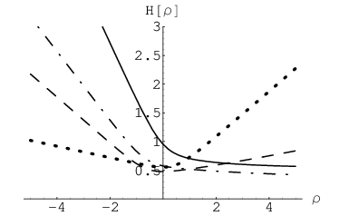
The constants $h_{1}$ , $C$ and $\phi_{0}$ are arbitrary. In particular $\phi_{0}$ can be fixed to any value. For what concerns $C$ and $h_{1}$ , instead, what happens is more interesting. While any choice of them gives a solution to equations (3.1) - (3.4), requiring that a particular solution behaves in the UV as the functions in section 3.1 imposes an additional condition that enforces a relation between the useful values of $C$ and $h_{1}$ . Figure 1 is the plot of such a relation for two fixed values of $\frac{N_{f}}{N_{c}}$ . All other possible choices still give a solution to (3.1) - (3.4), but the functions either reach a singularity at some finite value of $\rho$ or reach the UV with a different asymptotical behaviour, in which we are not interested here (analogous to the one studied in section 8 of [11]).

Refer to caption — Figure 1: We represent here the relationship between $C$ and $h_{1}$ that ensures that the evolution of a given type II expansion goes asymptotically to the behaviour we presented in section 3.1. On the left we are considering negative values of $C$ , corresponding to expansion (3.10) while on the right positive values are considered, which correspond to (3.11). Dashed lines correspond to $\frac{N_{f}}{N_{c}}=1.5$ while continuous lines correspond to $\frac{N_{f}}{N_{c}}=2.5$ .

3.2.3 Type III expansion

When the constant $C$ in (3.1) vanishes, type II expansions are not allowed anymore, but a new branch of solutions opens up, which we will call type III. In this case both $H$ and $G$ vanish at the origin of space. The expansion reads as follows

		$\displaystyle H=h_{1}\rho^{\frac{1}{3}}+\frac{1}{10}(5N_{c}-7N_{f})\rho+\frac{2}{3}h_{1}\rho^{\frac{4}{3}}+\ldots$
		$\displaystyle G=h_{1}\rho^{\frac{1}{3}}-\frac{1}{10}(5N_{c}+2N_{f})\rho+\frac{2}{3}h_{1}\rho^{\frac{4}{3}}+\ldots$
		$\displaystyle Y=\frac{h_{1}}{6}\rho^{-\frac{2}{3}}-\frac{N_{f}}{10}+\frac{4}{9}h_{1}\rho^{\frac{1}{3}}+\ldots$
		$\displaystyle\phi=\phi_{0}+\frac{3N_{f}}{8h_{1}}\rho^{\frac{2}{3}}+3\frac{10N_{c}^{2}-10N_{c}N_{f}+7N_{f}^{2}}{160h_{1}^{2}}\rho^{\frac{4}{3}}+\ldots$		(3.12)

Again the constants $h_{1}$ and $\phi_{0}$ are arbitrary, but to obtain a solution that asymptotes to the behaviour of section 3.1, we have to choose a particular value of $h_{1}$ for any fixed value of $\frac{N_{f}}{N_{c}}$ .

3.3 Numerical solutions

The expansions above are essential in the analysis of solutions to the system (3.1)-(3.4), but their knowledge is not enough to guarantee the existence of an overall solution that connects the given UV and IR behavior. We have checked that such connecting solution indeed exists for the three kinds of IR behaviours. In this section, we plot some sample numerical computations.

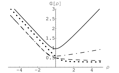
Figure 2 gives some examples of the numerical integration for the type I IR behaviour.

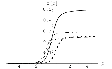
As we have already anticipated, requiring that the type II and III expansions are connected with the UV asymptotics of section 3.1 imposes an additional condition, fixing the value of the integration constant $h_{1}$ in terms of $C$ and $\frac{N_{f}}{N_{c}}$ . This additional condition produces the plots in Figure 1. Given that we choose the suitable value of $h_{1}$ , it is then possible to numerically integrate equations (3.1)-(3.4), and find a complete solution for the type A backgrounds. For type II and type III solutions, we present examples of these solutions in Figures 3 and 4, for different values of $C$ and $\frac{N_{f}}{N_{c}}$ .

3.4 UV expansions revisited

The reader may wonder how it is possible that different IR behaviours asymptote to the same UV when it seems that the UV expansions (3.5), (3.6) have no free parameters apart from $C$ . Indeed, those expansions are not complete and there is an extra free parameter in the UV if one considers the possibility of exponentially suppressed terms: we can write,

H=Q_{0}(\rho)+e^{-4\rho}\rho^{-\alpha}Q_{1}(\rho)+{\cal O}(e^{-8\rho})

(3.13)

where $Q_{0}$ are the expansions (3.5), (3.6) with:

	$\displaystyle\alpha=\frac{2N_{c}-3N_{f}}{3(2N_{c}-N_{f})}\qquad(N_{f}<2N_{c})$
	$\displaystyle\alpha=\frac{2N_{c}+N_{f}}{3(2N_{c}-N_{f})}\qquad(N_{f}>2N_{c})$		(3.14)

The $Q_{i}(\rho)$ are polynomials such that $Q_{i}(\rho)=Q_{i,0}+Q_{i,1}\rho^{-1}+Q_{i,2}\rho^{-2}+\dots$ . $Q_{1,0}$ is a free parameter and the rest are fixed in terms of it. We have, thus (once $C,N_{c},N_{f}$ are fixed), a one parameter family of UV solutions, labelled by $Q_{1,0}$ . Different choices $Q_{1,0}$ should modify the IR behaviour and, in particular, make the system fall into one of the qualitatively different IR possibilities. However, checking this numerically requires great numerical precision and we could not bear out this expectation explicitly.

It would be interesting to know the physical interpretation of this parameter $Q_{1,0}$ . Since it comes multiplying a term with $e^{-4\rho}$ , it must be related to the vacuum expectation value of an operator of UV dimension 6, here we anticipate the UV radius-energy relation $\log[\mu/\Lambda]=\frac{2}{3}\rho$ that we will use in equation (4.6). The simplest guess is an operator of the type $(Q\tilde{Q})^{4}$ (since in the UV $\gamma_{Q}\rightarrow-\frac{1}{2}$ , at least when $N_{f}\leq 2N_{c}$ ). A single vev of this type would spontaneously break the R-symmetry, apparently in contradiction with the described solution. However, since there are infinitely many smeared flavored branes in the construction, it is natural to think that, if in fact such vevs are turned on, they may also be smeared effectively restoring the $U(1)_{R}$ . This is similar to the discussion in [13] where, considering smeared masses for hypermultiplets, the R-symmetry that would be broken for a single mass is effectively restored.

3.5 A comment on integration constants

The different expansions are written in terms of some integration constants which are related among them. In order to avoid confusion, we clarify here the number of parameters on which the different families of solutions depend.

We have four first order equations (2.2)-(2.5). Let us fix $N_{f}/N_{c}$ (notice that, mantaining this ratio fixed, $N_{c}$ can be reabsorbed by simultaneously rescaling $H,G,Y$ ). Then a solution of the system depends on four integration constants. One is an additive constant for $\phi$ that does not affect the integration of the other functions. Since the BPS eqs do not depend explicitly on $\rho$ , a second integration constant is just a shift of $\rho$ , which we can fix without loss of generality. In type I, we can define $\rho=0$ as the point where $H^{\prime}$ (or $G^{\prime}$ ) vanishes, as in figure 2. For type II and III, we have defined $\rho=0$ as the point where $H$ (and/or $G$ ) vanish. The third integration constant is fixed by requiring that the system goes to the linear dilaton UV (so there are not growing exponentials in $H$ ). From the IR point of view, this is, for instance, what fixes $h_{1}$ in terms of $C$ in the type II IR expansions, see the discussion in section 3.2.2.

Thus, for fixed $N_{f}/N_{c}$ and fixing also the additive constant of $\phi$ , we are left with the fourth integration constant, which gives a one-parameter family of type I and type II solutions. For type III, where we further require $C=0$ , there is a single solution (a limiting point of the type II family).

After these discussions on the solutions, we will focus on obtaining physics predictions from them. To this we turn now.

4 Physics predictions of the new solutions

In this section, we study some non-perturbative aspects that can be learned from the solutions presented in section 3. We will discuss expressions for the gauge coupling and anomalous dimensions of the quark superfields, give predictions for their values and compute the beta function in the UV of the theory (matching results known from field theory). The predicted anomalous dimension for the quark superfield will be in agreement with the results of eq.(2.19) and those spelled out in section 2.3.1. We will present similar results for the beta function of the quartic coupling (for which we will provide a geometrical definition). We will study the Wilson and ’t Hooft loops and address in detail the issue of (continuous and discrete) anomaly matching.

Let us remind the reader that we take units so that $\alpha^{\prime}=g_{s}=1$ . With this choice, the tension of a D5 brane is $T_{5}=\frac{1}{(2\pi)^{5}}$ .

4.1 Theta-angle and gauge coupling

We will give an expression for the theta-angle and gauge coupling that can be simply derived by considering the action for a D5 brane on the submanifold $(t,\vec{x},\theta=\tilde{\theta},\varphi=2\pi-\tilde{\varphi})$ , at constant radial coordinate. This is a well known definition, originally proposed in [36]. In [11] we defined the gauge coupling using an instanton, whose action is computed using a D1 brane wrapping the two-cycle $(\theta=\tilde{\theta},\varphi=2\pi-\tilde{\varphi})$ . This two-manifold is special, being the only shrinking closed manifold in the geometry. As expected, the results using D5 or D1 probes do coincide.

We consider the dynamics of a D5 with gauge fields $A_{\mu}$ excited on the $R^{1,3}$ directions, obtaining (in string frame),

S_{D5}=-T_{5}\int d^{6}xe^{-\phi}\sqrt{-\det(g+2\pi F)}+\frac{1}{2}(2\pi)^{2}T_{5}\int C_{2}\wedge F_{2}\wedge F_{2}

(4.1)

The induced metric and two-form on the probe D5 brane read, in string frame,

	$\displaystyle ds^{2}_{ind}$	$\displaystyle=$	$\displaystyle e^{\phi}\Big[dx_{1,3}^{2}+(H+G)(d\theta^{2}+\sin^{2}\theta d\varphi^{2})\Big]\,,$
	$\displaystyle(C_{2})_{ind}$	$\displaystyle=$	$\displaystyle\frac{2N_{c}-N_{f}}{4}(\psi-\psi_{0})\sin\theta d\theta\wedge d\varphi$		(4.2)

Following the procedure of [36], we can expand (4.1) up to second order in the gauge fields (this is the QFT part of the $\alpha^{\prime}$ expansion), perform the integrals over the two-cycle and compare to the usual Yang-Mills action in order to obtain the couplings.

For the theta-angle, we get:

\Theta=\frac{(2N_{c}-N_{f})}{2}(\psi-\psi_{0}).

(4.3)

Since changes in $\Theta$ are associated with traslations $\psi\rightarrow\psi+2\epsilon$ then only some values of $\epsilon=\frac{2k\pi}{2N_{c}-N_{f}}$ are allowed and they correspond to changes in $\Theta\rightarrow\Theta+2k\pi$ , which nicely matches what we wrote about anomalies between eq.(2.23)-(2.25).

The gauge coupling in our SQCD theory takes the form,

\frac{8\pi^{2}}{g^{2}}=2(H+G).

(4.4)

For type I solutions, the series expansions of section 3.2.1 show that the gauge coupling vanishes in the IR. The expansions of section 3.2.2 for type II solutions show a version of ‘soft confinement’ (with bounded gauge coupling in the IR), while for type III more conventional confinement is obtained (with divergent gauge coupling in the IR). Figure 5 shows the behavior of the coupling as a function of the radial coordinate.

4.1.1 Beta Function and Anomalous Dimension

We can compute the beta function of the gauge coupling as defined in (4.4). As we stated below eq.(2.15), we will be interested in the wilsonian beta function, that takes the expression,

\beta_{\frac{8\pi^{2}}{g^{2}}}=\frac{\partial\Big(\frac{8\pi^{2}}{g^{2}}\Big)}{\partial\log(\mu/\Lambda)}=3N_{c}-N_{f}(1-\gamma_{Q}).

(4.5)

Now, we need a relation between the radial coordinate $\rho$ and the scale $\mu$ in order to perform the derivative in (4.5). In section 5.5 of [11] we proposed that the radius-energy relation, in the UV of the gauge theory, that is for large values of the radial coordinate, is:

\log[\mu/\Lambda]=\frac{2}{3}\rho\,\,,\qquad(\rm{UV},\,\rho\rightarrow\infty)

(4.6)

This relation was proved in the unflavored backgrounds by identifying the gaugino condensate (an operator of dimension 3) with a deformation of the background that asymptotically behaves as $e^{-2\rho}$ , see [36, 37]. Since in the flavored backgrounds, the same kind of deformation (leading to the type N solutions) still has the same exponential behaviour [11], (4.6) is trustable in the present setup.

We now proceed doing the computation (4.5) in the UV (for $\rho\rightarrow\infty$ ). After substituting (4.4), (4.6) and (2.2), (2.3), one obtains an expression for the anomalous dimension of the quark superfield $\gamma_{Q}$ in terms of the background functions,

\gamma_{Q}=\frac{12}{N_{f}}Y-\frac{1}{2}-3\frac{N_{c}}{N_{f}}\,\,,\qquad(\rm{UV},\,\rho\rightarrow\infty)

(4.7)

Inserting (3.5), we find the UV behaviour of the anomalous dimension for $N_{f}<2N_{c}$ :

\gamma_{Q}\sim-\frac{1}{2}-\frac{12N_{c}}{32(2N_{c}-N_{f})\rho^{2}}\,\,,\qquad(N_{f}<2N_{c})

(4.8)

This expression is quite nice, because it matches the fact that the anomalous dimensions of the quark superfield approaches $\gamma_{Q}=-\frac{1}{2}$ to have the R-charge $R[Q]=1/2$ , see the discussion in section 4.8.

One may wonder what happens in theories with $N_{f}>2N_{c}$ (which are Seiberg dual to those with $N_{c}<N_{f}<2N_{c}$ ). Introducing in (4.7) the expansion of $Y$ for $N_{f}>2N_{c}$ , eq. (3.6), we find:

\gamma_{Q}\sim\frac{5}{2}-6\frac{N_{c}}{N_{f}}-\frac{3(N_{f}-N_{c})}{8(N_{f}-2N_{c})\rho^{2}}\,\,,\qquad(N_{f}>2N_{c})

(4.9)

So $\gamma_{Q}>-\frac{1}{2}$ , as anticipated in section 2.2.2.

4.2 The quartic coupling

We will now analyze similar issues for the quartic coupling in the superpotential of (2.11). Let us start with the beta function.

4.2.1 Beta function of the quartic coupling

Let us go back to the field theory expression of the beta functions as we discussed them in eq.(2.18). We have, for the (dimensionless) quartic coupling:

\beta_{\tilde{\kappa}}=\frac{\partial\tilde{\kappa}}{\partial\log(\mu/\Lambda)}=\tilde{\kappa}(1+2\gamma_{Q})

(4.10)

Using the radius-energy relation (4.6) and the value of the anomalous dimension computed in (4.7), we find:

\frac{\partial\log\tilde{\kappa}}{\partial\rho}=\frac{2}{3}(1+2\gamma_{Q})=\frac{16Y}{N_{f}}-4\frac{N_{c}}{N_{f}}\,\,,\qquad(\rm{UV},\,\rho\rightarrow\infty)

(4.11)

So, in view of (2.3), we can identify:

\log\tilde{\kappa}=c+\frac{8G}{N_{f}}\,\,,\qquad(\rm{UV},\,\rho\rightarrow\infty)

(4.12)

where $c$ is some constant.

Let us analyze what happens with the quartic coupling when $N_{f}<2N_{c}$ and $N_{f}>2N_{c}$ . Whether it is relevant or irrelevant depends on the sign of $1+2\gamma_{Q}=\frac{6}{N_{f}}(4Y-N_{c})$ .

When $N_{f}<2N_{c}$ :

1+2\gamma_{Q}=-\frac{2N_{c}}{3(2N_{c}-N_{f})}\rho^{-2}<0

(4.13)

so the quartic coupling is relevant: starts at some constant in the UV and grows towards the IR.

When $N_{f}>2N_{c}$ ,

1+2\gamma_{Q}=\frac{6}{N_{f}}(N_{f}-2N_{c})>0

(4.14)

so the quartic is irrelevant and diverges in the UV. Notice the consistency of these results with the field theory discussion in [29, 38].

4.2.2 Geometric interpretation

In principle, one could expect that the quartic coupling could be read as data of the geometry, i.e. as some quotient of the volumes of the different cycles of the manifold. In that sense, (4.12) is not very satisfactory.

Without a definite understanding, we speculate in this section about a definition of the quartic coupling that makes use of the geometry of the internal manifold. Since (4.12) is trustable in the UV, we require that our guess behaves similarly in the large $\rho$ region. We start with the $N_{f}<2N_{c}$ in which the coupling is relevant and bounded in the UV:

\displaystyle\tilde{\kappa}=e^{c+\frac{8G}{N_{f}}}\approx 1+\frac{N_{c}}{2(2N_{c}-N_{f})}\rho^{-1}+\dots\,\,,\qquad(N_{f}<2N_{c})

(4.15)

where we have conveniently fixed $c$ (an overall factor) to make the expression simpler.

We will now propose a definition for the quartic coupling $\tilde{\kappa}$ in terms of the geometry. First, let us notice that, for fixed $\rho$ , we have one well defined two-cycle, a well defined one-cycle and a couple of well defined three-cycles. The two-cycle is the one mentioned before and given by

\hat{S}^{2}=[\theta=\tilde{\theta},\;\;\varphi=2\pi-\tilde{\varphi}],\;\;\;Vol[\hat{S}^{2}]=4\pi e^{\phi}(H+G).

(4.16)

The one-cycle, along the worldvolume of the flavor branes, is parametrized by the angle $\psi$ and its volume is

S^{1}=[\psi],\;\;Vol[S^{1}]=4\pi e^{\phi/2}\sqrt{Y}.

(4.17)

It is possible to define two different 3-cycles in the internal manifold

S^{3}=(\theta,\varphi,\psi),\;Vol[S^{3}]=(4\pi)^{2}e^{3/2\phi}H\sqrt{Y},\;\;\tilde{S}^{3}=(\tilde{\theta},\tilde{\varphi},\psi),\;\;Vol[\tilde{S}^{3}]=(4\pi)^{2}e^{3/2\phi}G\sqrt{Y}

(4.18)

We define the quartic coupling as a quotient of the volume of the two-cycle times the one-cycle divided by the volume of one of the three-cycles. This definition makes sense since the coupling we are interested in (relevant for matchings between string and gauge theory) must be adimensional:

\tilde{\kappa}=\frac{Vol[S^{1}]\times Vol[\hat{S}^{2}]}{Vol[S^{3}]}

(4.19)

Then:

\tilde{\kappa}=1+\frac{G}{H}=1+\frac{N_{c}}{2(2N_{c}-N_{f})}\rho^{-1}+\dots

(4.20)

When studying the Seiberg dual magnetic theory, one should change $S^{3}\rightarrow\tilde{S}^{3}$ according to the prescription (2.21). This amounts to the interchange $H\leftrightarrow G$ .

When $N_{f}>2N_{c}$ , the quartic coupling grows exponentially towards the UV and the definition (4.19) should be taken carefully. This is perhaps not surprising since the field theory description with a quartic term breaks down and needs some UV completion. We relegate further discussion to Appendix A.

4.3 A nice matching with the $N_{f}=2N_{c}$ case

In this section, we will show a connection between our solutions for $N_{f}<2N_{c}$ with the one for $N_{f}=2N_{c}$ and the one for $N_{f}>2N_{c}$ , and analyse it in view of the properties of the quartic coupling discussed above. We will need to use that all of the solutions are of the form (2.1), with the expansions in eqs.(3.5)-(3.6) and that for $N_{f}=2N_{c}$ an explicit solution is given by [11] ( $\xi$ is a free parameter valued in $0<\xi<4$ ),

H(\rho)=\frac{N_{c}}{\xi},\;\;\;G(\rho)=\frac{N_{c}}{4-\xi},\;\;\;Y=\frac{N_{c}}{4},\;\;\;\phi(\rho)=\phi_{0}+\rho.

(4.21)

We now consider the solution with $N_{f}<2N_{c}$ in the far UV ( $\rho\rightarrow\infty$ ), and change the number of flavors towards $N_{f}\rightarrow 2N_{c}^{-}$ with a particular scaling limit

\lim_{\rho\rightarrow\infty,\;\;N_{f}\rightarrow 2N_{c}^{-}}(2N_{c}-N_{f})\rho\rightarrow\infty,

(4.22)

so we have that the functions in eq.(3.5) behave as

H\approx\Big(\frac{2N_{c}-N_{f}}{2}\Big)\rho\rightarrow\infty,\;\;G\approx\frac{N_{c}}{4},\;\;\phi\approx\rho.

(4.23)

According to (4.12), the quartic coupling takes some finite value at this point.

We see that we can match this with the $N_{f}=2N_{c}$ solution (4.21) if we take $\xi=0$ . After matching, we move freely in the parameter $\xi$ (since in the $N_{f}=2N_{c}$ case, $\xi$ represents a marginal coupling [11]), from $\xi=0$ towards $\xi=4$ . At the point $\xi=4$ the functions take the values

G\rightarrow\infty,\;\;H=\frac{N_{c}}{4},\;\;\phi=\rho

(4.24)

and the quartic coupling diverges. We can match (4.24) with the expansion for $N_{f}>2N_{c}$ in eq.(3.6) if we scale similarly as above,

\lim_{\rho\rightarrow\infty,\;\;N_{f}\rightarrow 2N_{c}^{+}}(N_{f}-2N_{c})\rho\rightarrow\infty.

(4.25)

The interpretation is the following: since when $N_{f}>2N_{c}$ , the quartic is irrelevant, we can only connect those theories with the end of the $N_{f}=2N_{c}$ marginal line in which this coupling is infinite. On the other hand, when $N_{f}<2N_{c}$ , the quartic is relevant so these theories approach the conformal $N_{f}=2N_{c}$ point by the opposite limit of the marginal line, where the quartic takes its smallest value. At $N_{f}=2N_{c}$ , we can tune $\xi$ (accordingly changing the quartic coupling) to move from one end of the line to the other. The process continuously connects, in the space of theories, the $N_{f}<2N_{c}$ case to the $N_{f}>2N_{c}$ one.

This “flow in the number of flavors” provides a nice quantitative check and suggests that our discussion about the quartic coupling in section 4.2.1 is sensible. It would be nice to understand if similar matchings and flows may happen for different solutions with $N_{f}=2N_{c}$ [35].

Let us now study the potential between static quark-antiquark and monopole-antimonopole pairs, using Wilson and ’t Hooft loops.

4.4 Wilson Loop and QCD-string

In order to get some intuition of what will happen to the quark-antiquark pair when separated, we can analyze a quantity associated with the tension of the putative QCD-string that forms between them. The functional form of this tension (that can be thought of as the tension of an F1-string when taken to the IR of the background) is given by,

	$\displaystyle T_{Q\bar{Q}}\sim\sqrt{g_{tt}g_{xx}}\|_{IR}=e^{\phi}\|_{IR}$
	$\displaystyle T_{Q\bar{Q},{TypeI}}\rightarrow 0$
	$\displaystyle T_{Q\bar{Q},{TypeII}}\rightarrow e^{\phi_{0}}$
	$\displaystyle T_{Q\bar{Q},{TypeIII}}\rightarrow e^{\phi_{0}}$		(4.26)

$T_{Q\bar{Q}}$ gives a qualitative way of evaluating the tension in the IR dynamics. The expressions (4.26) tell us that type I solutions will have vanishing QCD-string tension (indicating that quarks are free), type II and type III solutions will show finite tension, indicating confinement. This is in agreement with the behavior of the gauge coupling in eq.(4.4). Of course, the presence of dynamical quarks will produce screening (string breaking) when the energy stored in the QCD-string (4.26) is of the order of the lightest meson in the theory.

Let us now compute the Wilson loop following the standard prescription of [39]. Consider the action for an F1 string parametrized by

t=\tau,\;\;x=\sigma,\;\;\rho=\rho(\sigma)

(4.27)

with $x$ taking values in $[0,L]$ (such that $\rho(0)=\rho(L)=\infty$ ) and $\tau$ in $[0,\infty)$ . The induced metric on this string is,

ds^{2}_{ind}=e^{\phi}\Big[-d\tau^{2}+(1+4Y{\rho^{\prime}}^{2})d\sigma^{2}\Big]

(4.28)

So, the Nambu-Goto action for this string is

S=\frac{1}{2\pi\alpha^{\prime}}\int d\sigma e^{\phi}\sqrt{1+4Y{\rho^{\prime}}^{2}}

(4.29)

This is in the form to follow the usual treatment for Wilson loops in [40], and write expressions for the (renormalized) energy $E$ and the separation $L$ . There is a one-parameter family of string profiles depending on the minimal value of $\rho$ reached by the string, which we call $\rho_{0}$ .

	$\displaystyle E(\rho_{0})=\frac{1}{2\pi\alpha^{\prime}}\left[e^{\phi(\rho_{0})}L+2\int_{\rho_{0}}^{\infty}2\sqrt{Y}(\sqrt{e^{2\phi}-e^{2\phi(\rho_{0})}}-e^{\phi})d\rho-2\int_{0}^{\rho_{0}}2\sqrt{Y}e^{\phi}d\rho\right]$
	$\displaystyle L(\rho_{0})=4e^{\phi(\rho_{0})}\int_{\rho_{0}}^{\infty}\sqrt{\frac{Y}{e^{2\phi}-e^{2\phi(\rho_{0})}}}d\rho$		(4.30)

These integrals can be studied numerically for our solutions. We will present an example in figure 6 at the end of the next section.

4.5 t’Hooft loop

It is interesting to perform a qualitative analysis similar to the one around eq.(4.26). In this case, the effective tension for the monopole-antimonopole pair is given by the effective tension of the magnetic string, represented by a D3-brane wrapping the two-cycle (4.16) and extended along $(x,t)$ stretched at the bottom of the geometry. See eq.(4.32) and below for details,

	$\displaystyle T_{m\bar{m}}\sim e^{\phi}(H+G)\|_{IR}$
	$\displaystyle T_{m\bar{m},{TypeI}}\rightarrow e^{\phi_{0}}N_{f}$
	$\displaystyle T_{m\bar{m},{TypeII}}\rightarrow e^{\phi_{0}}C$
	$\displaystyle T_{m\bar{m},{TypeIII}}\rightarrow 0$		(4.31)

$T_{m\bar{m}}$ gives a qualitative way of evaluating the tension of the monopole-antimonopole pair in the IR dynamics Intuitively, eq. (4.31) indicates that type I and type II solutions confine the monopoles, while type III solutions exhibit free monopoles.

Let us now study in detail the t’ Hooft loop that can be thought of as the “Wilson loop for magnetic monopoles”(the rigorous definition is in terms of the commutation relations with the Wilson loop operator). It is a similar computation to the one for the Wilson loop in the previous section, as we explained above, for a extended wrapped D3 brane on the cycle $\Sigma_{4}$ ,

\Sigma_{4}=\Big(t=\tau,\;\;x_{1}=\sigma,\;\;\;\rho(\sigma),\;\;\theta=\tilde{\theta},\;\;\varphi=2\pi-\tilde{\varphi}\Big).

(4.32)

This gives an induced metric that in string frame reads,

ds_{ind}^{2}=e^{\phi}\Big[-dt^{2}+(1+4Y{\rho^{\prime}}^{2})d\sigma^{2}+(H+G)(d\theta^{2}+\sin^{2}\theta d\varphi^{2})\Big]

(4.33)

and the action (per unit time) for the ‘effective string’ obtained after integrating out the two-cycle is,

S=4\pi T_{3}\int d\sigma\sqrt{\hat{f}^{2}+\hat{g}^{2}{\rho^{\prime}}^{2}},\;\;\;\hat{f}=e^{\phi}(H+G),\;\;\;\hat{g}=2\hat{f}\sqrt{Y}

(4.34)

We observe that this expression is “Seiberg invariant” according to the definition (2.20), and analogous formulas to those in eqs. (4.30) can be used. They read

	$\displaystyle L(\rho_{0})=2\int_{\rho_{0}}^{\infty}\frac{\hat{g}}{\hat{f}}\frac{\hat{f}(\rho_{0})}{\sqrt{\hat{f}^{2}(\rho)-\hat{f}^{2}(\rho_{0})}}d\rho\quad$
	$\displaystyle E=4\pi T_{3}\left[\hat{f}(\rho_{0})L+2\int_{\rho_{0}}^{\infty}\frac{\hat{g}(\rho)}{\hat{f}(\rho)}\Big({\sqrt{\hat{f}^{2}(\rho)-\hat{f}^{2}(s_{0})}}-\hat{f}(\rho)\Big)d\rho-2\int_{0}^{\rho_{0}}\hat{g}(\rho)d\rho\right]\quad$		(4.35)

An example of numerical analysis for the expressions (4.35) using the functions (4.34) is plotted in figure 6.

Our interpretation of figure 6 is as follows: first, it is interesting to notice that the graphs for the backgrounds with different IR behaviours share some qualitative properties, suggesting a smooth interpolation among the different solutions. In all cases, there is a maximum length reached by the loop which we interpret as string breaking due to pair creation. ⁵⁵ 5 In [41], it was argued in a similar situation that such kind of behaviour did not correspond to string breaking. Moreover, in both graphs, there is a line (the type III one for the Wilson loop and the one corresponding to type I for the ’t Hooft loop) which stretches more than the rest indicating linear confinement (before the string is eventually broken). This qualitatively suggests a change of roles of quarks and monopoles between type I and type III backgrounds. We will elaborate on this in the next section. Finally, let us point out that there are also minimal lengths in the graphs. Presumably, this is due to the growing linear dilaton, which signals the failure of the supergravity description we are using at asymptotically large $\rho$ . With such an UV completion, there should be a minimal length ( $L_{min}$ ) of the field theory that can be reliably probed by the present computation. Indeed, the converging growing lines on the left of the ’t Hooft loop graph are an artifact of this UV behaviour (length and energy in equations (4.35) grow with $\rho_{0}$ when $\rho_{0}$ is taken large). Thus, we discard this part of such lines as unphysical. The fact that the type III line of the ’t Hooft loop graph only follows this unphysical behaviour indicates that in the corresponding field theory, monopoles are free (or they are screened at a length shorter than $L_{min}$ ).

We close this section with a technical comment about the obtention of the graphs in figure 6. In order to compare the loops probing the different solutions, one has to ensure that they asymptote to the same UV (once we fix the additive constant of integration $\phi_{0}$ for one of the solutions, the $\phi_{0}$ of the rest have to be fixed accordingly). It is also necessary to take into account that having $C\neq 0$ , the UV behaviour of $H$ is different from the $C=0$ case (see eq(3.5)). Thus, in order to compare with other solutions, the definition of the coordinate $\rho$ has to be shifted $\rho\rightarrow\rho-\frac{2C}{2N_{c}-N_{f}}$ (so the origin of space is not at $\rho=0$ any more).

4.6 Back to the 1970’s

Briefly, we want to make contact with the material in section 2.4.

The intuitive analysis for the string tensions in eq.(4.26) and eq.(4.31), shows that in the three types of IR solutions the behavior for the potential between the (non-dynamical) quark-antiquark and monopole-antimonopole pair is quite diverse. Indeed, the intuitive analysis presented around eqs.(4.26)-(4.31) shows that for small separations compared to the mass of a pair, type I solutions confine monopoles and let quarks move freely. The opposite occurs in solutions of type III, while type II solutions present a situation in which quarks and monopoles experience a growing force when separated ⁶⁶ 6 We emphasize again that for long distances pair creation gives place to string breaking and the law changes..

Another important observation is the fact that one can smoothly interpolate between the solutions of types I, II and III by changing the values of the integration constants. Indeed, one can see that in the limit of vanishing constant $C$ in type II solutions (see section 3.2.2), the expansions change into those of type III in section 3.2.3 (this was repeatedly stressed when plotting the functions). The connection with type I solutions in section 3.2.1 must be thought in a more heuristic way, by noticing that if the constants $C$ and $h_{1}$ in the type II solutions were absent the expansions could continue past $\rho=0$ to smaller values of the radial coordinate and the leading term in the expansion would go like the type I solutions (this connection could be made more precise in terms of the UV constants of integration $C,Q_{1,0}$ , see section 3.4, but this is hard to see in the numerical analysis).

This ‘heuristic matching’ resembles the fact that in theories with fundamental fields there are no phase transitions in moving between a confining and a higgsed situation [33]. The different VEV’s of the operator of dimension six mentioned in section 3.4 is what should take the theory from one vacua (a particular string background) to another. Together with the behavior for Wilson and ’t Hooft loops, this leads us to propose that the solutions of type I, II and III behave like the Higgs, oblique confined and confined regimes of the SQCD-like theory in eq.(2.11). In the oblique confined phase, some dyons condense and become free. This should be achieved in the present setup by the vanishing tension of a wrapped extended D3-brane with some F-strings disolved inside it, i.e. with the worldvolume electric field turned on. We leave this computation for the future.

The qualitative picture described above is quite appealing. However, we should write here a word of caution. The tensions (4.26) and (4.31) depend on a combination of functions at the singularity; even when the singular behavior cancels from the expressions of (4.26) and (4.31) -a manifestation of the ‘good’ character of the singularity- these results should be taken with care. It could happen that the criterion we are using for ‘good singularities’ is not enough and that not all the discussed solutions should be accepted as physical.

None of the described behaviours corresponds to an IR conformal fixed point. We remind the reader that SQCD with a quartic superpotential flows in the IR to Seiberg’s conformal fixed point of SQCD [29] (at least in the ratio $N_{f}/N_{c}$ appropriate to fall in the conformal window). We believe that this does not show up in our set-up since, as explained in section 2.2.1, the theory dual to the string solution differs from the usual SQCD+quartic near the IR, presumably due to a non-trivial VEV.

4.7 A comment on the running couplings

Coming back to the expressions for the Wilson and ’t Hooft loops in eqs.(4.29)-(4.34), we observe that they are invariant under the Seiberg duality transformation (2.20). Even more, one can easily see that the gauge coupling defined in eq.(4.4) is also invariant. This may puzzle the reader, who may expect that while the electric theory is strongly coupled in the IR, the magnetic theory should be IR free and vice versa. This is not what we observe; our solutions predict that both theories are strongly coupled (or both have weak $g_{YM}^{2}$ coupling) towards the IR. This situation is not totally original, it is indeed what happens inside the conformal window in Seiberg’s SQCD. In contrast, in our case, we do not have a conformal window, but we will see that having two theories with similar IR behavior is not ruled out.

Let us discuss this issue using the expressions for the wilsonian beta function in eq.(4.5) and the values for the anomalous dimensions we obtained in eqs.(4.8)-(4.9) for the $N_{f}<2N_{c}$ and $N_{f}>2N_{c}$ cases respectively. First, we introduce the notation: the theory $\bf{e}$ is the one with gauge group $SU(N_{c})$ and $N_{f}$ flavors. We will assume that in the $\bf{e}$ theory $N_{f}<2N_{c}$ , and the superpotential is,

{\cal{W}}_{e}=\kappa_{e}\Big(\tilde{Q}Q\tilde{Q}Q-\frac{1}{N_{c}}(\tilde{Q}Q)^{2}\Big)

(4.36)

We will denote by m theory the one obtained by Seiberg duality from the theory e. The m theory will have gauge group $SU(n_{c})$ with $N_{f}$ flavors, of course the relation is $n_{c}=N_{f}-N_{c}$ . This, together with the fact that in the e theory we set $N_{f}<2N_{c}$ implies that $N_{f}>2n_{c}$ in the theory m. The superpotential in the m theory is (we will ignore, since it plays no role, the double trace term),

{\cal{W}}_{m}=\hat{\kappa}_{m}MM+\frac{1}{\mu}\tilde{q}Mq

(4.37)

where we have used that the new fields in the Seiberg dual theory are the meson $M_{ij}$ (not charged under the $SU(n_{c})$ gauge field $w_{\alpha}$ ), the quarks $q$ and the antiquarks $\tilde{q}$ .

Now, let us compute the beta functions in each theory. For this, we will need to know the anomalous dimensions of the fields. Our solutions predict (in the UV) anomalous dimensions for the e quarks $\gamma_{Q}$ and the m quarks $\gamma_{q}$ given by eqs.(4.8) and (4.9)

	$\displaystyle\gamma_{Q}=\frac{12}{N_{f}}Y-\frac{1}{2}-3\frac{N_{c}}{N_{f}}\sim-\frac{1}{2}-\frac{12N_{c}}{(64N_{c}-32N_{f})\rho^{2}}$
	$\displaystyle\gamma_{q}=\frac{12}{N_{f}}Y-\frac{1}{2}-3\frac{n_{c}}{N_{f}}\sim\frac{5}{2}-6\frac{n_{c}}{N_{f}}-\frac{3(N_{f}-n_{c})}{(8N_{f}-16n_{c})\rho^{2}}.$		(4.38)

Let us neglect the small $O(\rho^{-2})$ correction in the far UV ( $\rho\rightarrow\infty$ region), keeping only the leading terms. Now, we compute the beta functions. We use the values for the anomalous dimensions in eq.(4.38), obtaining that the wilsonian beta functions for the two theories are given by,

	$\displaystyle\beta_{\frac{8\pi^{2}}{g_{e}^{2}}}=3N_{c}-N_{f}(1-\gamma_{Q})=\frac{3}{2}(2N_{c}-N_{f}),$
	$\displaystyle\beta_{\frac{8\pi^{2}}{g_{m}^{2}}}=3n_{c}-N_{f}(1-\gamma_{q})=\frac{3}{2}(N_{f}-2n_{c}),$
			(4.39)

This shows that either both the electric and magnetic theories confine or they both are IR free. The result in eq.(4.39) is precisely the one we obtain if we use the UV expansions for $H(\rho),G(\rho)$ in section 3.1 together with eqs.(4.7)-(4.9). We now move to the matching of anomalies.

4.8 Global Anomaly matching

In a field theory like SQCD or ours in eq.(2.11) there are two types of currents, global (denoted below by $j_{g}$ ) and local or gauge currents, denoted by $J_{L}$ . Hence, there are four possible 3-point correlators of currents one may compute

	$\displaystyle<J_{L}J_{L}J_{L}>,$		(4.40)
	$\displaystyle<j_{g}j_{g}J_{L}>,$		(4.41)
	$\displaystyle<j_{g}J_{L}J_{L}>,$		(4.42)
	$\displaystyle<j_{g}j_{g}j_{g}>.\;\;$		(4.43)

The first and second correlators (4.40)-(4.41) must be zero, or the gauge symmetry is anomalous and the theory is inconsistent.

The correlator with two local currents in eq.(4.42) if nonzero, indicates the presence of an anomaly in the global current $<\partial_{\mu}j^{\mu}_{g}>\neq 0$ . While for non-anomalous symmetries in the sense of eq.(4.42), the correlator for three global currents in eq.(4.43) must match in the two descriptions of the theory. This is the ’t Hooft anomaly matching condition.

We will start by studying the anomaly for the $R$ symmetry current, as expressed by the correlator in (4.42), and related to the results of sections 2.3.1 and 4.1. This is what appears in the changes for the $\Theta$ angle. A general expression for this anomaly is,

\psi\rightarrow e^{i\epsilon\gamma_{5}}\psi,\;\;\;\Delta\Theta=\epsilon\sum_{r}n_{r}T(r)R[\psi]

(4.44)

where the $\psi$ denotes the massless fermions of the theory, $n_{r}$ is the number of particles in the $r$ representation of the gauge group, $T(r)$ is the weight of the representation (we remind the reader that $T(adj)=2N_{c},\;T(fund)=1$ ) and $R[\psi]$ is the R-charge of the corresponding fermion. We need to assign R-symmetry charges to the superfields. The gaugino has $R[\lambda]=1$ and we want to determine the R-charges of the fundamental superfields. They cannot be read directly from the supergravity solution, but they can be extracted indirectly from the $\Theta$ -angle transformation. Let us start looking at the electric e-theory (with $N_{f}<2N_{c}$ ). From (4.44), we read (using $R[\psi_{Q}]=R[\psi_{\tilde{Q}}]$ , required by the symmetry):

\Delta\Theta_{e}=\epsilon_{e}(2N_{c}+2N_{f}R[\psi_{Q}])

(4.45)

The values of $\epsilon_{e}$ that leave $\Theta_{e}$ invariant (modulo $2\pi$ ) are written in (2.25) and immediately suggest $R[\psi_{Q}]=-\frac{1}{2}$ . Thus, we are led the following assignation (for the fermions in the multiplet) under the global symmetry $SU(N_{f})_{V}\times U(1)_{B}\times U(1)_{R}$ , for the electric e-theory:

\psi_{Q}=(N_{f},1,-1/2),\;\;\psi_{\tilde{Q}}=(\bar{N}_{f},-1,-1/2),\;\;\lambda=(1,0,1)

(4.46)

This implies that for the scalars of the quark multiplets $R[Q]=R[\tilde{Q}]=\frac{1}{2}$ . Notice that this is consistent with the existence of the quartic superpotential preserving the R-symmetry at the classical level. Let us also discuss the relation of this R-charge to the anomalous dimension of the quark field. At a conformal point

dimO=\frac{3}{2}R[O]

(4.47)

Using this relation and the UV value of the anomalous dimension of the squark (4.8), we find $R[Q]=\frac{2}{3}dim[Q]=\frac{2}{3}(1+\frac{1}{2}\gamma_{Q})=\frac{1}{2}$ , in agreement with the discussion above. The relation (4.47) can be used here because our theory has an asymptotic UV fixed point (the beta-function for the gauge coupling becomes trivially zero since the gauge coupling itself goes to zero and the one for the quartic coupling also vanishes due to $\gamma_{Q}=-\frac{1}{2}$ , see (4.10)).

We now turn to the dual magnetic m-theory with $n_{c}=N_{f}-N_{c}$ colors such that $N_{f}>2n_{c}$ . We denote the magnetic quarks with lower case $q$ . In this case, (4.44) yields:

\Delta\Theta_{m}=\epsilon_{m}(2n_{c}+2N_{f}R[\psi_{q}])

(4.48)

Comparison to (2.25) again suggests $R[\psi_{q}]=-\frac{1}{2}$ , which we believe is the charge relevant to the backgrounds discussed in this paper. However, there is another logical possibility which we find interesting and we will discuss it in section 4.8.1. Therefore, we consider the following charges for the magnetic m-theory:

	$\displaystyle\psi_{q}=(\bar{N}_{f},\frac{N_{c}}{n_{c}},-\frac{1}{2}),\;\;\psi_{\tilde{q}}=(N_{f},-\frac{N_{c}}{n_{c}},-\frac{1}{2})$
	$\displaystyle\psi_{M}=(N_{f}\times\bar{N}_{f},0,0),\;\;\tilde{\lambda}=(1,0,1)$		(4.49)

This implies that for the scalars of the quark multiplets $R[q]=R[\tilde{q}]=\frac{1}{2}$ and for the meson multiplet $R[M]=1$ , again allowing the superpotential to preserve the R-symmetry. However, given (4.9), one can see that the relation (4.47) is not satisfied. This should not come as a surprise, because the quartic coupling grows in the UV of the magnetic theory, see around eq.(4.14) and the UV theory is far from a conformal point.

Indeed, now that the assignations in eqs.(4.46),(4.49) have been given, the next step is to check whether ’t Hooft matching in the sense of eq.(4.43) holds. Since the R-symmetry is anomalous, the continuous global symmetry is $SU(N_{f})_{V}\times U(1)_{B}$ . The triangles that should be matched are,

<SU(N_{f})_{V}^{3}>,\;\;<SU(N_{f})_{V}^{2}U(1)_{B}>,\;\;<U(1)_{B}^{3}>,\;\;<U(1)_{B}TT>

(4.50)

where the last triangle representes the ‘gravitational anomaly’ with two insertions of $T_{\mu\nu}$ . Let us quote the results in the e theory with the values of eq.(4.46), we denote $d^{ABC}=Tr(T^{A}[T^{B},T^{C}])$ ,

	$\displaystyle<SU(N_{f})_{V}^{3}>=d^{ABC}N_{f}N_{c}(1^{3}+(-1)^{3})=0$
	$\displaystyle<SU(N_{f})_{V}^{2}U(1)_{B}>=tr(T^{A}T^{B})2N_{f}N_{c}(1-1)=0$
	$\displaystyle<U(1)_{B}^{3}>=N_{f}N_{c}(1^{3}+(-1)^{3})=0$
	$\displaystyle<U(1)_{B}TT>=N_{f}N_{c}(1-1)=0$		(4.51)

while for the m theory, with values (4.49), we have

	$\displaystyle<SU(N_{f})_{V}^{3}>=d^{ABC}N_{f}n_{c}(1^{3}+(-1)^{3})=0$
	$\displaystyle<SU(N_{f})_{V}^{2}U(1)_{B}>=tr(T^{A}T^{B})2N_{f}n_{c}(\frac{N_{c}}{n_{c}}-\frac{N_{c}}{n_{c}})=0$
	$\displaystyle<U(1)_{B}^{3}>=N_{f}n_{c}[(\frac{N_{c}}{n_{c}})^{3}+(-\frac{N_{c}}{n_{c}})^{3}]=0$
	$\displaystyle<U(1)_{B}TT>=N_{f}n_{c}(\frac{N_{c}}{n_{c}}-\frac{N_{c}}{n_{c}})=0$		(4.52)

We see that there is anomaly matching between the electric and magnetic descriptions, satisfying ’t Hooft criteria. Up to here, the computation is identical to that for the usual ${\cal N}=1$ SQCD without superpotential. In [42], it was shown in that triangles involving discrete symmetries should also be matched. It is therefore a non-trivial consistency check to compute the values involving the remnant non-anomalous R-symmetry $Z_{2N_{c}-N_{f}}=Z_{N_{f}-2n_{c}}$ .

We now explicitly check the matching of discrete anomalies between the electric and magnetic description. Following the paper [42], we can compute the values for the triangles involving the R-symmetry. There is a technical subtlety explained in [42]. We need to have integer values for the different charges to match discrete anomalies, so they have to be rescaled. Thus, following the prescription in [42], we consider a $Z_{k}=Z_{4N_{c}-2N_{f}}$ R-symmetry. The baryonic and R-charges are ‘rescaled’ with respect to the values in the e-theory eq.(4.46) for the fermion in the multiplet and read:

\psi_{Q}=(N_{f},\frac{N_{f}-N_{c}}{n},-1),\;\;\psi_{\tilde{Q}}=(\bar{N}_{f},-\frac{(N_{f}-N_{c})}{n},-1),\;\;\lambda=(1,0,2)

(4.53)

while for the dual theory m, rescaling in the same fashion the values in eq.(4.49), we have

	$\displaystyle\psi_{q}=(\bar{N}_{f},\frac{N_{c}}{n},-{1}),\;\;\psi_{\tilde{q}}=(N_{f},-\frac{N_{c}}{n},-{1})$
	$\displaystyle\psi_{M}=(N_{f}\times\bar{N}_{f},0,0),\;\;\tilde{\lambda}=(1,0,2)$		(4.54)

The integer $n$ is defined as the greatest common divisor of $N_{c}$ and $N_{f}$ :

n\equiv GCD(N_{c},N_{f})

(4.55)

One has to study the following triangles:

<Z_{k}TT>,\;\;<Z_{k}U(1)_{B}^{2}>,\;\;<Z_{k}^{3}>,\;\;<SU(N_{f})^{2}Z_{k}>

(4.56)

We will consider the difference between the triangles in the electric and the magnetic theory. They should match up to multiples of $k=4N_{c}-2N_{f}$ [42]. We obtain the following results,

	$\displaystyle<Z_{k}TT>_{e}=2N_{c}N_{f}(-1)+2(N_{c}^{2}-1),\;\;<Z_{k}TT>_{m}=2n_{c}N_{f}(-1)+2(n_{c}^{2}-1),$
	$\displaystyle\Delta(e-m)=0$		(4.57)

which is a multiple of $k=4N_{c}-2N_{f}$ as required by [42].

For the second triangle involving three ‘discrete’ currents,

	$\displaystyle<Z_{k}^{3}>_{e}=2N_{c}N_{f}(-1)^{3}+8(N_{c}^{2}-1),\;\;<Z_{k}^{3}>_{m}=2n_{c}N_{f}(-1)^{3}+8(n_{c}^{2}-1),$
	$\displaystyle\Delta(e-m)=6N_{f}(2N_{c}-N_{f}).$		(4.58)

Again, the difference is a multiple of $k$ . For the triangle involving two baryonic and a ‘discrete’ current,

	$\displaystyle<Z_{k}U(1)_{B}^{2}>_{e}=2N_{c}N_{f}\left(\frac{N_{f}-N_{c}}{n}\right)^{2}(-1),\;\;<Z_{k}U(1)_{B}^{2}>_{m}=2n_{c}N_{f}(-1)\left(\frac{N_{c}}{n}\right)^{2},$
	$\displaystyle\Delta(e-m)=2\frac{N_{c}N_{f}}{n^{2}}(N_{f}-N_{c})(2N_{c}-N_{f}),$		(4.59)

we obtain the correct matching modulo $k$ ; finally for the triangle involving the non-abelian global symmetry

	$\displaystyle<SU(N_{f})^{2}Z_{k}>_{e}=-2N_{c}N_{f}\;\;<SU(N_{f})^{2}Z_{k}>=-2n_{c}N_{f}$
	$\displaystyle\Delta(e-m)=-2N_{f}(2N_{c}-N_{f}),$		(4.60)

We see that the assignation of charges appropriately rescaled (4.53), (4.54) satisfies the discrete anomaly matching up to multiples of $k=(4N_{c}-2N_{f})$ as explained in [42]. This nice match indicates that the value for the R-charge suggested by the string background is consistent with the field theory computations using the charges in eqs. (4.46),(4.49).

4.8.1 A different charge assignation

We again consider the charges for the electric theory written in (4.46), but give different R-charges for the magnetic theory. Coming back to (4.48), a second possibility to match the supergravity result (2.25) is to take $R[\psi_{q}]=\frac{1}{2}-2\frac{n_{c}}{N_{f}}$ .

Our second assignation of charges for the magnetic theory under the symmetries is, thus (like before, we give the charge of the fermions in the multiplet):

	$\displaystyle\psi_{q}=(\bar{N}_{f},\frac{N_{c}}{n_{c}},\frac{1}{2}-2\frac{n_{c}}{N_{f}}),\;\;\psi_{\tilde{q}}=(N_{f},-\frac{N_{c}}{n_{c}},\frac{1}{2}-2\frac{n_{c}}{N_{f}})$
	$\displaystyle\psi_{M}=(N_{f}\times\bar{N}_{f},0,-2+4\frac{n_{c}}{N_{f}}),\;\;\tilde{\lambda}=(1,0,1)$		(4.61)

The nice thing about this second assignation is that it satisfies the relation in eq.(4.47), as can be checked by using (4.9) (although, as explained above, there is no reason to expect (4.47) to hold out of a conformal point). The downside is that this implies that the coupling $\hat{\kappa}_{m}$ in eq.(4.37) must be charged, so the R-symmetry is completely broken at the classical level in the magnetic theory. This could only correspond to the dual of an electric theory in which the R-symmetry is spontaneously broken and, thus, it does not seem relevant to the type A backgrounds discussed in this paper. We believe that this second assignation could describe a situation like what happens for type N background in eq.(2.6) or those solutions found in [11], which will have the same UV as our type A backgrounds. Since in this case there is no remnant R-symmetry, an anomaly matching computation as the one in (4.56)-(4.60) does not apply.

In summary, to match in field theory the R-symmetry anomalies to the ones computed by the string solutions, we proposed values for the charges of the multiplets under the global and discrete symmetries. Notice that the R-charges are checked by the string background in the sense that the anomaly is encoded in the background via the potential $C_{(2)}$ (see section 2.3.1). Both charge assignations we have given are consistent with this computation. On the other hand, the charges under $SU(N_{f})$ and $U(1)_{B}$ written above are suggested by field theory considerations but not from the actual string solution. However, it is remarkable that the string solution indirectly knows about them (at least in the case of assignation (4.46),(4.49)) throught the discrete anomaly matching computation displayed in eqs. (4.56)-(4.60). The results in this section together with the previous checks, make us very confident of the interpretations that we have put forward for the string background.

5 Summary, conclusions and future directions

Let us briefly summarize the different topics elaborated in this paper. We have found a set of solutions for backgrounds of type A in eq.(2.1), proposed to be dual to a version of ${\cal N}=1$ SQCD (2.11). With the new solutions, we predicted the behavior for different field theory observables and phenomena like Seiberg duality, gauge coupling and its running, Wilson and ’t Hooft loops, anomalous dimensions of the quark superfields, quartic coupling, its running and anomalies (continuous and discrete). Based on those string theory predictions, we provided a large number of matchings between field theory expectations and string theory results. Interestingly, our solutions seem to realize the Fradkin-Shenker result for the non-existence of phase transitions when moving between higgsed and confining phases of a theory with fundamental fields [33].

This work leaves some open questions for future research. Indeed, it should be nice, among other things, to understand if the same ‘phase structure’ occurs in type N backgrounds in eq.(2.6) and the behavior of the quartic coupling in that case. The picture of Seiberg duality for type N backgrounds could be understood on a similar way as we did in this paper. The case of massive flavors, either for type A or N backgrounds also presents interest because it gives a resolution of the IR (good) singularity and its many applications. These and other topics will be dealt with in [24].

It should also be interesting to apply our treatment for quartic couplings to cascading theories. Sorting out other dynamical aspects of the backgrounds presented here, like for example, the spectrum of glueballs, mesons and baryons [43] is of main interest. The Veneziano expansion we are adopting indicates that there will be interactions leading to decays between the first two types of excitations and suggests ways to study baryons as solitons in the BI-WZ action.

It should also be interesting to extend all this story to the type II A case, using backgrounds like the ones in [44]. Extensions to lower dimensional field theories may prove interesting for condensed matter problems. Finally, it should be nice to think about possible high energy phenomenology applications of this line of research.

Acknowledgments:

In the last year or so, discussions with different colleagues have shaped our understanding and the presentation of the topics in this paper. For those discussions, we would like to thank: Gert Aarts, Riccardo Argurio, Adi Armoni, Francesco Benini, Francesco Bigazzi, Aldo Cotrone, Felipe Canoura, Stefano Cremonesi, Justin Foley, Seba Franco, Simon Hands, Prem Kumar, Biagio Lucini, Asad Naqvi, Alfonso V. Ramallo and Diego Rodriguez Gómez. RC and AP are supported by European Commission Marie Curie Postdoctoral Fellowships under contracts MEIF-CT-2005-024710 and MEIF-CT-2005-023373. RC and AP’s work was also partially supported by INTAS grant, 03-51-6346, RTN contracts MRTN-CT-2004-005104 and MRTN-CT-2004-503369, CNRS PICS # 2530, 3059 and 3747, and by a European Union Excellence Grant, MEXT-CT-2003-509661.

APPENDIX

Appendix A Beta function for $\kappa_{m}$

The computation of the beta function for the quartic coupling in the magnetic case seems to be tricky, so, here we will write the results we get and our interpretation.

If we Seiberg dualize the coupling $\kappa_{e}$ in eq.(4.20) we get the magnetic version $\kappa_{m}=1+\frac{H}{G}$ . We compute the beta function from string theory using the radius-energy relation eq.(4.6) and we obtain

\frac{1}{\kappa_{m}}\beta_{\tilde{\kappa}_{m}}=\frac{\partial\log[\tilde{\kappa}_{m}]}{\partial\log(\frac{\mu}{\Lambda})}=\frac{3}{2}\frac{\partial}{\partial\rho}\log\Big(1+\frac{H}{G}\Big)\approx-\frac{3}{4}\frac{(N_{f}-n_{c})}{(N_{f}-2n_{c})\rho^{2}}.

(A.1)

Now, let us look at the QFT results. The superpotential after Seiberg duality is given by,

{\cal{W}}_{m}=\hat{\kappa}MM+\hat{z}\tilde{q}Mq

(A.2)

The classical dimensions for fields and couplings are,

[q]=m,\;\;[M]=m,\;\;[\hat{\kappa}]=m,\;\;[\hat{z}]=1

(A.3)

where we used that the “meson” $M$ is a fundamental field in the magnetic theory and not a composite of electric quarks. The R-charges of fields and couplings, obtained from the main part of the paper eqs.(4.61) ⁷⁷ 7 For the values of R-charges in eqs.(4.46)-(4.49) we cannot find an expression for the anomalous dimension of the meson superfield. We are not at a conformal point and the relation (4.47) should not be used. are,

R[q]=(\frac{3}{2}-2\frac{n_{c}}{N_{f}}),\;\;R[M]=(4\frac{n_{c}}{N_{f}}-1),\;\;R[\hat{\kappa}]=4(1-2\frac{n_{c}}{N_{f}})

(A.4)

and the anomalous dimensions from the main part of the paper (for the meson it is computed assuming that the relation between dimension and R-charge is the one of a fixed point),

\gamma_{q}=\frac{12}{N_{f}}Y-\frac{1}{2}-3\frac{n_{c}}{N_{f}}\approx\frac{5}{2}-6\frac{n_{c}}{N_{f}}-\frac{3}{8}\frac{(N_{f}-n_{c})}{(N_{f}-2n_{c})\rho^{2}},\;\;\;\gamma_{M}=-5+12\frac{n_{c}}{N_{f}}

(A.5)

We can now compute

\beta_{\hat{\kappa}}=\hat{\kappa}[-1+\gamma_{M}]=\hat{\kappa}(12\frac{n_{c}}{N_{f}}-6),\;\;\;\beta_{\hat{z}}=\hat{z}[\gamma_{q}+\frac{1}{2}\gamma_{M}]=-\frac{3}{8}\hat{z}\Big(\frac{N_{f}-n_{c}}{(N_{f}-2n_{c})\rho^{2}}\Big)

(A.6)

On the other hand, we could have considered the superpotential after integration out of the massive meson in eq.(A.2)

{\cal{W}}_{m}=\tilde{\delta}\tilde{q}q\tilde{q}q

(A.7)

where the double trace term is present but has no relevance here. In this case the beta function from QFT has the expression,

\beta_{\tilde{\delta}}=\tilde{\delta}[1+2\gamma_{q}]=(6-12\frac{n_{c}}{N_{f}})+\frac{3}{4}\frac{(N_{f}-n_{c})}{(N_{f}-2n_{c})\rho^{2}}

(A.8)

It seems that the string theory computation in eq.(A.1) is reproducing the beta function of a combination of field theory couplings in eq.(A.6) and eq.(A.8). Indeed, the R-symmetry neutral combination that makes this work is $\kappa_{m}=(\delta\hat{\kappa})^{-1}.$

References

[1] J. M. Maldacena, Adv. Theor. Math. Phys. 2, 231 (1998) [Int. J. Theor. Phys. 38, 1113 (1999)] [arXiv:hep-th/9711200].
[2] S. S. Gubser, I. R. Klebanov and A. M. Polyakov, Phys. Lett. B 428, 105 (1998) [arXiv:hep-th/9802109]. E. Witten, Adv. Theor. Math. Phys. 2, 253 (1998) [arXiv:hep-th/9802150].
[3] N. Itzhaki, J. M. Maldacena, J. Sonnenschein and S. Yankielowicz, Phys. Rev. D 58, 046004 (1998) [arXiv:hep-th/9802042].
[4] G. ’t Hooft, Nucl. Phys. B 72, 461 (1974). G. ’t Hooft, Nucl. Phys. B 75, 461 (1974).
[5] L. Girardello, M. Petrini, M. Porrati and A. Zaffaroni, Nucl. Phys. B 569, 451 (2000); hep-th/9909047. L. Girardello, M. Petrini, M. Porrati and A. Zaffaroni, JHEP 9905, 026 (1999); hep-th/9903026. J. Polchinski and M. J. Strassler, hep-th/0003136. J. Babington, D. E. Crooks and N. J. Evans, Phys. Rev. D 67, 066007 (2003); hep-th/0210068. I. R. Klebanov and M. J. Strassler, JHEP 0008, 052 (2000); hep-th/0007191.
[6] A. Karch and E. Katz, JHEP 0206, 043 (2002) [arXiv:hep-th/0205236]. M. Kruczenski, D. Mateos, R. C. Myers and D. J. Winters, JHEP 0307, 049 (2003) [arXiv:hep-th/0304032]. M. Kruczenski, D. Mateos, R. C. Myers and D. J. Winters, JHEP 0405, 041 (2004) [arXiv:hep-th/0311270]. J. Babington, J. Erdmenger, N. J. Evans, Z. Guralnik and I. Kirsch, Phys. Rev. D 69, 066007 (2004) [arXiv:hep-th/0306018]. C. Nunez, A. Paredes and A. V. Ramallo, JHEP 0312, 024 (2003) [arXiv:hep-th/0311201]. D. Mateos, R. C. Myers and R. M. Thomson, Phys. Rev. Lett. 97, 091601 (2006) [arXiv:hep-th/0605046]. T. Albash, V. G. Filev, C. V. Johnson and A. Kundu, arXiv:hep-th/0605088. T. Sakai and S. Sugimoto, Prog. Theor. Phys. 113, 843 (2005) [arXiv:hep-th/0412141]. R. Apreda, J. Erdmenger, D. Lust and C. Sieg, JHEP 0701, 079 (2007) [arXiv:hep-th/0610276]. C. Sieg, JHEP 0708, 031 (2007) [arXiv:0704.3544 [hep-th]].
[7] F. Karsch, Lect. Notes Phys. 583, 209 (2002) [arXiv:hep-lat/0106019]. P. Giudice and S. Hands, Nucl. Phys. B 789, 111 (2008) [arXiv:hep-lat/0703001].
[8] G. Veneziano, Nucl. Phys. B 117, 519 (1976). G. C. Rossi and G. Veneziano, Nucl. Phys. B 123, 507 (1977). G. Veneziano, “The Color And Flavor Of 1/N Expansions,” CERN-TH-2311, May 1977. 21pp
[9] B. A. Burrington, J. T. Liu, L. A. Pando Zayas and D. Vaman, JHEP 0502, 022 (2005) [arXiv:hep-th/0406207]. I. Kirsch and D. Vaman, Phys. Rev. D 72, 026007 (2005) [arXiv:hep-th/0505164]. J. Erdmenger and I. Kirsch, JHEP 0412, 025 (2004) [arXiv:hep-th/0408113].
[10] I. R. Klebanov and J. M. Maldacena, Int. J. Mod. Phys. A 19, 5003 (2004) [arXiv:hep-th/0409133]. F. Bigazzi, R. Casero, A. L. Cotrone, E. Kiritsis and A. Paredes, JHEP 0510, 012 (2005) [arXiv:hep-th/0505140]. R. Casero, A. Paredes and J. Sonnenschein, JHEP 0601, 127 (2006) [arXiv:hep-th/0510110].
[11] R. Casero, C. Nunez and A. Paredes, Phys. Rev. D 73, 086005 (2006) [arXiv:hep-th/0602027].
[12] R. Casero and A. Paredes, Fortsch. Phys. 55, 678 (2007) [arXiv:hep-th/0701059].
[13] A. Paredes, JHEP 0612, 032 (2006) [arXiv:hep-th/0610270].
[14] F. Benini, F. Canoura, S. Cremonesi, C. Nunez and A. V. Ramallo, JHEP 0702, 090 (2007) [arXiv:hep-th/0612118]. F. Benini, F. Canoura, S. Cremonesi, C. Nunez and A. V. Ramallo, JHEP 0709, 109 (2007) [arXiv:0706.1238 [hep-th]]. F. Benini, arXiv:0710.0374 [hep-th].
[15] B. A. Burrington, V. S. Kaplunovsky and J. Sonnenschein, arXiv:0708.1234 [hep-th].
[16] G. Bertoldi, F. Bigazzi, A. L. Cotrone and J. D. Edelstein, Phys. Rev. D 76, 065007 (2007) [arXiv:hep-th/0702225]. A. L. Cotrone, J. M. Pons and P. Talavera, JHEP 0711, 034 (2007) [arXiv:0706.2766 [hep-th]].
[17] S. Hirano, JHEP 0705, 064 (2007) [arXiv:hep-th/0703272]. See Also: Sebastian Franco, Diego Rodriguez-Gomez and Hermann Verlinde, to appear.
[18] P. Koerber and D. Tsimpis, JHEP 0708, 082 (2007) [arXiv:0706.1244 [hep-th]].
[19] J. M. Maldacena and C. Nunez, Phys. Rev. Lett. 86, 588 (2001) [arXiv:hep-th/0008001].
[20] A. H. Chamseddine and M. S. Volkov, Phys. Rev. Lett. 79, 3343 (1997) [arXiv:hep-th/9707176]. A. H. Chamseddine and M. S. Volkov, Phys. Rev. D 57, 6242 (1998) [arXiv:hep-th/9711181].
[21] R. P. Andrews and N. Dorey, Phys. Lett. B 631, 74 (2005) [arXiv:hep-th/0505107]. R. P. Andrews and N. Dorey, Nucl. Phys. B 751, 304 (2006) [arXiv:hep-th/0601098].
[22] U. Gursoy and C. Nunez, Nucl. Phys. B 725, 45 (2005) [arXiv:hep-th/0505100].
[23] R. Casero, E. Kiritsis and A. Paredes, Nucl. Phys. B 787, 98 (2007) [arXiv:hep-th/0702155].
[24] Roberto Casero, Carlos Nunez and Angel Paredes, in preparation.
[25] I. Affleck, M. Dine and N. Seiberg, Nucl. Phys. B 241, 493 (1984).
[26] G. Carlino, K. Konishi and H. Murayama, JHEP 0002, 004 (2000) [arXiv:hep-th/0001036]. K. Hori, H. Ooguri and Y. Oz, Adv. Theor. Math. Phys. 1, 1 (1998) [arXiv:hep-th/9706082]. V. Balasubramanian, B. Feng, M. x. Huang and A. Naqvi, Annals Phys. 310, 375 (2004) [arXiv:hep-th/0303065].
[27] R.Argurio, F.Bigazzi, A. Cotrone, L. Martucci and C. Nunez. In preparation. See also the talk by Carlos Nunez in http://www.solvayinstitutes.be/Activities/WorkshopGaugeTheories/Talks.html
[28] N. Seiberg, Nucl. Phys. B 435, 129 (1995) [arXiv:hep-th/9411149]. K. A. Intriligator and N. Seiberg, Nucl. Phys. Proc. Suppl. 45BC, 1 (1996) [arXiv:hep-th/9509066].
[29] M. J. Strassler, arXiv:hep-th/0505153.
[30] U. Gursoy, S. A. Hartnoll and R. Portugues, Phys. Rev. D 69, 086003 (2004) [arXiv:hep-th/0311088].
[31] G. ’t Hooft, Nucl. Phys. B 138, 1 (1978). S. Mandelstam, Phys. Lett. B 53, 476 (1975).
[32] G. ’t Hooft, Phys. Scripta 25 (1982) 133. G. ’t Hooft, Nucl. Phys. B 190, 455 (1981).
[33] E. H. Fradkin and S. H. Shenker, Phys. Rev. D 19, 3682 (1979).
[34] J. M. Maldacena and C. Nunez, Int. J. Mod. Phys. A 16, 822 (2001) [arXiv:hep-th/0007018].
[35] E. Caceres, R. Flauger, M. Ihl and T. Wrase, arXiv:0711.4878 [hep-th].
[36] P. Di Vecchia, A. Lerda and P. Merlatti, Nucl. Phys. B 646, 43 (2002) [arXiv:hep-th/0205204]. M. Bertolini and P. Merlatti, Phys. Lett. B 556, 80 (2003) [arXiv:hep-th/0211142].
[37] R. Apreda, F. Bigazzi, A. L. Cotrone, M. Petrini and A. Zaffaroni, Phys. Lett. B 536, 161 (2002) [arXiv:hep-th/0112236].
[38] M. J. Strassler, arXiv:hep-th/0309149.
[39] J. M. Maldacena, Phys. Rev. Lett. 80, 4859 (1998) [arXiv:hep-th/9803002]. S. J. Rey and J. T. Yee, Eur. Phys. J. C 22, 379 (2001) [arXiv:hep-th/9803001].
[40] J. Sonnenschein, arXiv:hep-th/0003032.
[41] R. Apreda, D. E. Crooks, N. J. Evans and M. Petrini, JHEP 0405, 065 (2004) [arXiv:hep-th/0308006].
[42] C. Csaki and H. Murayama, Nucl. Phys. B 515, 114 (1998) [arXiv:hep-th/9710105].
[43] E. Caceres and C. Nunez, JHEP 0509, 027 (2005) [arXiv:hep-th/0506051]. M. Berg, M. Haack and W. Muck, Nucl. Phys. B 736, 82 (2006) [arXiv:hep-th/0507285]. M. Berg, M. Haack and W. Muck, Nucl. Phys. B 789, 1 (2008) [arXiv:hep-th/0612224].
[44] M. Atiyah, J. M. Maldacena and C. Vafa, J. Math. Phys. 42, 3209 (2001) [arXiv:hep-th/0011256]. J. D. Edelstein and C. Nunez, JHEP 0104, 028 (2001) [arXiv:hep-th/0103167]. A. Brandhuber, J. Gomis, S. S. Gubser and S. Gukov, Nucl. Phys. B 611, 179 (2001) [arXiv:hep-th/0106034]. M. Cvetic, G. W. Gibbons, H. Lu and C. N. Pope, Phys. Lett. B 534, 172 (2002) [arXiv:hep-th/0112138].