Lüscher-Weisz algorithm for excited states of the QCD flux-tube
Abstract:
We present a version of the Lüscher-Weisz multilevel algorithm ideally suited for studying excited states of the QCD flux tube. While the original version achieved error reduction only in the temporal direction, the new algorithm reduces fluctuations in the sources as well. We report on the implementation of this algorithm as well as improvement over the older method. We also present first results, where we see a good agreement with theoretical predictions from bosonic string models.
July 30 - August 4 2007
Regensburg, Germany
1 Introduction
Formation of a flux-tube between a quark and an antiquark in the QCD vacuum plays an important role in the description of the still unsolved phenomenon of quark confinement. At a large distance between the quarks, it is believed that the QCD flux tube has quite a similar behavior to an oscillating bosonic string, largely independent of the internal gluonic degrees of freedom which make up the flux tube.
This led to the formulation of effective string theories for the flux tube [1] and a lot of studies have dealt with the groundstate of the string [2]. The simplest model describing the excited states of the string is that of the free bosonic string. A more realistic model is provided by the Nambu string theory. An important development by Arvis [3] was the writing down of a potential assuming the flux tube to be described by a Nambu string.
Nevertheless the Nambu theory still has the conformal anomaly in anything other than 26 dimensions. This has led to several other proposals for effective string theories. Lüscher and Weisz [4] imposed an open- closed duality on the string partition function and obtained the Nambu string spectrum up to order . Another effective string theory introduced by Polchinski and Strominger [5] consists of the most general terms at every order in , which does not introduce the conformal anomaly. In this theory too the string spectrum agrees with Arvis up to corrections of order [6]. For a recent review see [7].
In this article we look at the excitation spectrum of the flux tube formed between a static quark and an antiquark in 3 dimensional SU(2) lattice gauge theory and compare our results with the predictions for open bosonic string spectra. For a similar study in the closed string sector see [8].
2 Sources and excited states
In 2+1 dimensions, the energy states of the oscillating string can be classified by parity and charge-conjugation properties, , and one can identify the ground states in these channels with the lowest four energy states of the string:
| (1) |
Our goal is now to measure these energy states on the lattice.
The groundstate of the potential can be measured well with Polyakov loop correlators, which have the spectral representation In this case the coefficients are integers and are the energy states at quark separation . Effective string prediction for ground state is
| (2) |
where is an unphysical constant and is the string tension. The term is the well known Lüscher-term [9], reproduced by all effective string theories. Different models however give different predictions for the excitation spectrum and therefore one way to distinguish between different string-models is to measure the energy-differences between the excited states.
The Polyakov loop correlators used to calculate the groundstate of the potential are bad estimators for the excited states. A better way of measuring the excited states is provided by Wilson loops. However normal Wilson loops, with straight spatial lines at the ends, will again project strongly on the ground state, but weakly on the excited states. In order to get a preferential coupling to the excited states, we use a set of wavefunctions at the ends of the loops, called sources. These sources correspond to spatial lines on the lattice, that replace the straight spatial lines of the Wilson loops. The set of sources we use is shown in figure (1).


If one creates superpositions of these sources with well defined parity and charge conjugation, these ‘channels’ couple directly to the excited states according to equation 1. The superpositions are shown in table (1).
| channel | superposition | state | sources | time tr. | sources | time tr. | ||
|---|---|---|---|---|---|---|---|---|
| 4 | 12000 | 1000 | 24000 | 1000 | ||||
| 6 | 12000 | 1500 | 24000 | 2000 | ||||
| 8 | 12000 | 2000 | 24000 | 6000 | ||||
| 12000 | 2500 | 24000 | 12000 |
There have been other attempts to measure the excited states. Juge, Kuti and Morningstar [10] used asymmetric lattices with small physical temporal extent and a large number of basis states to measure the excited states in different field theories. In that respect our approach is complementary to theirs, as we use relatively few basis states, but use much larger physical temporal extents to exponentially suppress the contamination due to excited states.
We can now calculate the expectation values of Wilson loops with channel at the ends, which has the representation:
| (3) |
Thus we are able to measure the different energy states with the formula:
| (4) |
The “” in this expression are due to the higher states in the channel and, as can be seen from equation (3) are exponentially damped with and . This is why one would like to go to Wilson loops with large time extends.
The problem with large Wilson loops is of course the very small signal to noise ratio.
Even for the numerical cheap LGT in d=2+1, conventional methods do not work. One way of reducing the error is provided by the Lüscher-Weisz algorithm [11], which leads to an exponential error reduction for the time transporters of the Wilson loops. Putting the sources on fixed time-slices of the lattice and using the sublattice updates to reduce the fluctuations of the time transporters produces good results and is practicable for loops with time extends up to about a Fermi, see [12].
However this is not the best way to use the algorithm because the fluctuations of the sources are not reduced with this method.
3 The new method
To achieve further error reduction we now move the sources from the fixed lines to the middle of the time slices. Such a Wilson loop with sources at the ends is also shown in figure (1).
Main advantages of such a procedure are:
- •
The fluctuations of the sources are reduced by the sublattice updates as well.
- •
One can use multihit on single links of the sources that leads to a further error reduction.
It is also beneficial to use different numbers of sublattice updates for the time slices that contain the sources and the time slices that contain only time-transporters. In this way it is possible to choose parameters for the algorithm to optimize the noise to speed ratio for the single parts of the Wilson loops.
Several tests show, that it is good to use more sublattice updates for the sources than for the time transporters for excited states. If one chooses the right parameters for the sources and the time slices, one is able to achieve an error reduction of for the same computation time.
A related algorithm was used by Kratochvila and de Forcrand to look at string breaking with Wilson loops [13].
4 First results
In our first run we worked on a -lattice for and on a -lattice for , with (), made 2000 total measurements using the scheme of sublattice updates shown in table (1). Compared to [12] we were able to increase the time extent of the loops from to .
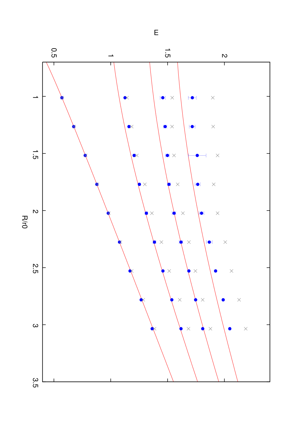
The naive energies are calculated with the formula:
| (5) |
To get rid of the contamination due to the higher states in the channels, we use a fit to the form
| (6) |
with the fit parameters to calculate the corrected energy . For the corrected energies and we were only able to use Wilson loops with the time extends . For the first two states we used Wilson loops with all time extents. The values we obtained are given in table(2).
| 4 | 0.5725(3) | 0.571(1) | 1.143(2) | 1.126(3) | 1.541(9) | 1.46(3) | 1.90(8) | 1.72(4) |
|---|---|---|---|---|---|---|---|---|
| 5 | 0.6776(4) | 0.674(2) | 1.184(2) | 1.161(3) | 1.540(8) | 1.48(2) | 1.90(7) | 1.72(3) |
| 6 | 0.7801(6) | 0.775(2) | 1.230(2) | 1.206(4) | 1.557(8) | 1.50(2) | 1.94(9) | 1.76(8) |
| 7 | 0.8826(9) | 0.8781(6) | 1.300(3) | 1.252(8) | 1.589(9) | 1.51(2) | 1.91(6) | 1.77(3) |
| 8 | 0.983(2) | 0.9779(8) | 1.362(3) | 1.31(2) | 1.635(10) | 1.56(2) | 1.94(7) | 1.80(3) |
| 9 | 1.085(2) | 1.0772(10) | 1.446(4) | 1.38(2) | 1.69(1) | 1.62(2) | 2.01(8) | 1.87(3) |
| 10 | 1.1847(4) | 1.170(5) | 1.5146(8) | 1.459(3) | 1.745(3) | 1.688(6) | 2.06(2) | 1.923(7) |
| 11 | 1.2862(4) | 1.268(4) | 1.6070(9) | 1.537(4) | 1.809(3) | 1.747(5) | 2.13(2) | 1.989(7) |
| 12 | 1.3858(5) | 1.364(6) | 1.6841(10) | 1.618(4) | 1.877(4) | 1.809(5) | 2.19(2) | 2.047(6) |

Even more interesting than the total energy values are the energy differences. Again to take the corrections into account, we use a three-parameter fit
| (7) |
with the parameters . The corresponding values are shown in table (3).
| 4 | 5 | 6 | 7 | 8 | 9 | 10 | 11 | 12 | |
|---|---|---|---|---|---|---|---|---|---|
| 0.551(4) | 0.478(5) | 0.426(4) | 0.378(7) | 0.341(10) | 0.31(2) | 0.287(3) | 0.267(3) | 0.250(3) | |
| 0.92(2) | 0.83(2) | 0.75(1) | 0.66(2) | 0.61(2) | 0.57(2) | 0.294(2) | 0.273(3) | 0.256(3) | |
| 1.15(3) | 1.04(3) | 0.99(8) | 0.89(3) | 0.82(2) | 0.79(3) | 0.753(9) | 0.721(8) | 0.683(9) |
5 Conclusions
We have discussed an algorithm that allows us to use the advantage of the Lüscher-Weisz algorithm for the time transporters as well as for the sources and we presented our first results using the algorithm. We were able to go to much bigger Wilson loops than was possible previously. We see from figure (3) that at the same separation the energy difference is much closer to the predictions from Arvis than the energy differences and , which agrees with the expactations in [4]. Also the magnitude of the corrections seems to be larger for the higher states. Unfortunately the error reduction obtained with the naive states is not sufficient to get a signal for the third excited state beyond . At the moment it is not clear whether this is due to lack of statistics or poor choice of parameters in the multilevel algorithm. Investigation into this issue is ongoing.
Acknowledgments.
All results were obtained employing the condor sytem 11 1 Copyright: 1990-2007 Condor-Team, Computer Sciences Department, University of Wisconsin – Madison, WI. [14] to make efficient use of the computing resources of the Westfälische Wilhelms-Universität Münster. We are thankful to the university for this facility.References
- [1] P. Goddard, J. Goldstone, C.Rebbi, C. Thorn, Quantum dynamics of a massless relativistic string, Nucl. Phys. B56, 109
- [2]
M. Lüscher, K. Symanzik, P. Weisz, Anomalies of the free loop wave equation in the WKB approximation, Nucl. Phys. B173, 365
L. Griffiths, C. Michael, P. Rakow, Mesons with excited glue, Phys. Lett. B129, 351
J. Stack, Heavy quark potential in SU(2) lattice gauge theory, Phys. Rev. D27, 412
N. Campbell, C. Michael, P. Rakow, The string tension from lattice QCD, Phys. Lett. B139, 288
Ph. de Forcrand, G. Schierholz, H. Schneider, M. Teper, The string and its tension in SU(3) lattice gauge theory: towards definitive results, Phys. Lett. B160, 137
N. Campbell, A. Huntley, C. Michael, Heavy quark potentials and hybrid mesons from SU(3) lattice gauge theories, Nucl. Phys. B306, 51 - [3] J.F. Arvis, The exact -potential in Nambu string theory, Phys. Lett. 127B, 106
- [4] M. Lüscher, P. Weisz, String excitation energies in SU(N) gauge theories beyond the free string approximation, JHEP 07 2004 014
- [5] J. Polchinski, A. Strominger, Effective string theory, Phys. Rev. Lett. 67 1991 1681.
- [6]
J. Drummond, Universal subleading spectrum of effective string theory, hep-th/0411017
N. Hari Dass, P. Matlock, Universality of correction to Lüscher term in Polchinski-Strominger effective string theories, hep-th/0606265
F. Maresca, Comparing the excitations of the periodic flux tube with effective string models, Ph.D. thesis, Trinity College, Dublin, 2004 - [7] J. Kuti, Lattice QCD and string theory, \posPoS(LAT2005)001
- [8]
A. Athenodorou, The spectrum of closed loops of fundamental flux in D=2+1 SU(N) gauge theories, \posPoS(Lattice2007)288
B. Bringholtz, M. Teper, Strings in SU(N) gauge theories in 2+1 dimensions: beyond the fundamental representation, \posPoS(Lattice2007)291 - [9] M. Lüscher, Symmetry-breaking aspects of the roughening transition in gauge theories, Nucl. Phys. B180, 317
- [10]
J. Juge, J. Kuti, C. Morningstar, Excitations of the static quark-antiquark system in several gauge-theories, hep-lat/0312019
J. Juge, J. Kuti, C. Morningstar, QCD string formation and the casimir energy, hep-lat/0401032 - [11] M. Lüscher, P. Weisz, Locality and exponential error reduction, JHEP 09 2001 010
- [12] P. Majumdar, The string spectrum from large Wilson loops, Nucl. Phys. B664, 213 [hep-lat/0211038]
- [13] S. Kratochvila, Ph. de Forcrand, Observing string breaking withWilsonn loops, Nucl. Phys. B671, 103 [hep-lat/0306011]
- [14] http://www.condorproject.org/