Low Dimensional Embedding of fMRI datasets Thanks: Submitted to Neuroimage, Sep. 2007. Revised Jan. 2008.
Abstract
We propose a novel method to embed a functional magnetic resonance imaging (fMRI) dataset in a low-dimensional space. The embedding optimally preserves the local functional coupling between fMRI time series and provides a low-dimensional coordinate system for detecting activated voxels. To compute the embedding, we build a graph of functionally connected voxels. We use the commute time, instead of the geodesic distance, to measure functional distances on the graph. Because the commute time can be computed directly from the eigenvectors of (a symmetric version) the graph probability transition matrix, we use these eigenvectors to embed the dataset in low dimensions. After clustering the datasets in low dimensions, coherent structures emerge that can be easily interpreted. We performed an extensive evaluation of our method comparing it to linear and nonlinear techniques using synthetic datasets and in vivo datasets. We analyzed datasets from the EBC competition obtained with subjects interacting in an urban virtual reality environment. Our exploratory approach is able to detect independently visual areas (V1/V2, V5/MT), auditory areas, and language areas. Our method can be used to analyze fMRI collected during “natural stimuli”.
Keywords:
fMRI, Laplacian eigenmaps, embedding, natural stimuli.1 Introduction
At a microscopic level, a large number of internal variables associated with various physical and physiological phenomena contribute to dynamic changes in functional magnetic resonance imaging (fMRI) datasets. FMRI provides a large scale (as compared to the scale of neurons) measurement of neuronal activity, and we expect that many of these variables will be coupled resulting in a low dimensional set for all possible configurations of the activated fMRI signal. We assume therefore that activated fMRI time series can be parametrized by a small number of variables. This assumption is consistent with the usage of low dimensional parametric models for detecting activated voxels (Petersson et al. 1999). This assumption is also consistent with the empirical findings obtained with principal components analysis (PCA) and independent components analysis (ICA) (B.B.Biswal and Ulmer 1999; McKeown et al. 2003), where a small number of components are sufficient to describe the variations of most activated temporal patterns. Both PCA and ICA make very strong assumptions about the components: orthogonality and statistical independence, respectively. Such constraints are convenient mathematically but have no physiological justification, and complicate unnecessarily the interpretation of the components (Friston 1998). A second limitation of PCA and ICA is that both methods only provide a linear decomposition of the data (Friston 2005). There is no physiological reason why the fMRI signal should be a linear combination of eigen-images or eigen-time series. In practice, the first components identified by PCA are often related to physiological artifacts (e.g. breathing), or coherent spontaneous fluctuations (Raichle and Mintun 2006). These artifacts can be responsible for most of the variability in the dataset. Stimulus triggered changes, which are much more subtle, rarely appear among the first components.
The contribution of this paper is a novel exploratory method to construct an optimal coordinate system that reduces the dimensionality of the dataset while preserving the functional connectivity between voxels (Sporns et al. 2000). First, we define a distance between time series that quantifies the functional coupling (Fox et al. 2005), or connectivity between the corresponding voxels. We then construct an embedding that preserves this functional connectivity across the entire brain. After embedding the dataset in a lower dimensional space, time series are clustered into coherent groups. This new parametrization results in a clear separation of the time series into: (1) response to a stimulus, (2) coherent physiological signals, (3) artifacts, and (4) background activity. We performed an extensive evaluation of our method comparing it to linear and nonlinear techniques using synthetic datasets and in vivo datasets.
2 Methods
2.1 Overview of our approach
Our goal is to find a new parametrization of an fMRI dataset, effectively replacing the time series by a small set of features, or coordinates, that facilitate the identification of task-related hemodynamic responses to the stimulus. The new coordinates will also be able to reveal the presence of physical or physiological processes that have an intrinsic low dimension. Such processes can be described with a small number of parameters (dimensions) in an appropriate representation (set of basis functions). These time series should be contrasted with noise time series that have a very diffuse representation in any basis. Example of such low-dimensional processes include task-related hemodynamic responses, non-task-related physiological rhythms (breathing and heart beating motion). We expect that only a small fraction of all time series will have a low-dimensional representation. The remaining time series will be engaged in a spontaneous intrinsic activity (Raichle and Mintun 2006). We call these time series background time series. As shown in our experiments, background time series are more complex, and cannot be well approximated with a small number of parameters.
We now introduce some notations that will be used throughout the paper. Let denote an fMRI dataset composed of scans, each comprised of voxels, which is represented as a matrix,
| (1) |
Row of is the time series generated from voxel . Column is the scan unrolled as a vector. In this work, we regard as a point in , with coordinates.
We seek a new parametrization of the dataset that optimally preserves the local functional coupling between time series. Most methods of reduction of dimensionality used for fMRI are linear: each is projected onto a set of components . The resulting coefficients serve as the new coordinates in the low dimensional representation. However, in the presence of nonlinearity in the organization of the in , a linear mapping may distort local functional correlations. This distortion will make the clustering of the dataset more difficult. Our experiments with in vivo data confirm that the subsets formed by the low-dimensional time series have a nonlinear geometry and cannot be mapped onto a linear subspace without significant distortion. We propose therefore to use a nonlinear map to represent the dataset in low dimensions. Because the map is able to preserve the local functional coupling between voxels, low dimensional coherent structures can easily be detected with a clustering algorithm. Finally, the temporal and the spatial patterns associated with each cluster are examined and the cluster that corresponds to the task-related response is identified. In summary, our approach includes the following three steps:
- 1.
Low dimensional embedding of the dataset;
- 2.
Clustering of the dataset using the new parameterization;
- 3.
Identification of the set of activated time series.

2.2 The connectivity graph: a network of functionally correlated voxels
In order to construct the nonlinear map we need to estimate the functional correlation between voxels. We characterize the functional correlation between voxels with a network. Similar networks have been constructed to study functional connectivity in (Achard et al. 2006; Caclin and Fonlupt 2006; Eguíluz et al. 2005; Fox et al. 2005; Sporns et al. 2000). We represent the network by a graph that is constructed as follows. The time series originating from voxel becomes the node (or vertex) of the graph11 1 We slightly abuse notation here: is a time series, as well as a node on the graph.. Edges between vertices quantify the functional connectivity. Each node is connected to its nearest neighbors according to the Euclidean distance between the time series, (Fig. 1). The weight on the edge quantifies the functional proximity between voxels and and is defined by
| (2) |
The scaling factor modulates the definition of proximity measured by the weight (2). If is very large, then for all the nearest neighbors of , we have (see (2)), and the transition probability is the same for all the neighbors, . This choice of promotes a very fast diffusion of the random walk through the dataset, and blurs the distinction between activated and background time series. On the other hand, if is extremely small, then for all the neighbors such that . Only if the distance between and is zero (or very small) the transition probability is non zero. This choice of accentuates the difference between the time series, but is more sensitive to noise. In practice, we found that the universal choice
where (we used for all experiments) is usually optimal.
The weighted graph is fully characterized by the weight matrix with entries . Let be the diagonal degree matrix with entries . The spatial coordinates of the voxels and are currently not used in the computation of . We know that spatial information can be useful: truly activated voxels tend to be spatially clustered. However, spatial proximity should be measured along the cortical ribbon, and not in the 3-D volume.
2.3 A new way to measure functional distances between voxels
Once the network of functionally connected voxels is created, we need to define a distance between any two vertices and in the network. This distance should reflect the topology of the graph, but should also be able to distinguish between strongly connected vertices (when the voxels and belong to the same functional region) and weakly connected vertices (when and have similar time series and , but belong to different functional regions). The Euclidean distance that is used to construct the graph is only useful locally: we can use it to compare voxels that are functionally similar, but we should use a different distance to compare voxels that may not be functionally similar. As shown in the experiments, the shortest distance between two nodes and measured along the edges of the graph is very sensitive to short-circuits created by the noise in the data. A standard alternative to the geodesic distance is the commute time, , that quantifies the expected path length between and for a random walk started at (Bremaud 1999).
We review here the concept of commute time in the context of a random walk on a graph. We show how the commute time can be computed easily from the eigenvectors of . Let us consider a random walk on the connectivity graph. The walk starts at , and evolves on the graph with the transition probability ,
| (3) |
If the walk is at , it jumps to one of the nearest neighbors, , with probability . The walk first visits all voxels in the same functional area before jumping to a different functional area. Indeed, if voxel and are in the same functional area, and voxel is in a different functional area, then we expect that , and therefore . This observation can be quantified by computing the average hitting time that measures the number of steps that it takes for the random walk started at to hit for the first time (Bremaud 1999),
The hitting time is not symmetric, and cannot be a distance on the graph. A proper distance is provided by a symmetric version of , called the commute time, (Bremaud 1999),
| (4) |
As one would expect, increases with the geodesic distance . Unlike the geodesic distance, decreases when the number of paths between the nodes increases.
Commute time and clustering coefficient
The commute time is greatly influenced by the richness of the connections
between any two nodes of the network. This concept can be quantified by the
clustering coefficient. Let be a node with neighbors. The
neighbors of may, or may not, be neighbors of one another. To asses
the transitivity of the connections, we can compute the total number of
edges, , that exist between all the neighbors of . The
clustering coefficient (Albert and Barabási 2002) is .
The maximum value of is and is achieved when each neighbor of
is connected to all the other neighbors of (they form a
clique). If the average clustering coefficient, computed over all nodes of
the network, is close to 1, then there will always be multiple routes
between any two nodes and , and the commute time will
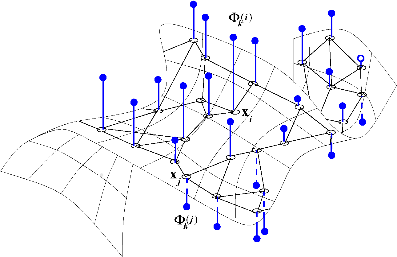
remain small. Eguíluz et al. 2005 measured clustering coefficients in networks of functionally connected voxels in fMRI that were indicative of scale-free small-world networks. Achard et al. 2006 identified networks of richly connected hubs in the cortex, and have also shown that the functional network (as measured by fMRI) exhibits the “small world” property. The commute time provides a distance on the graph that takes into account the abundance of connections that may exist between two nodes of the graph.
A spectral decomposition of commute time
As explained in the Appendix, the commute time can be conveniently computed
from the eigenvector of the symmetric matrix
. The corresponding
eigenvalues are between and , and can be labeled such that . Each eigenvector
is a vector with coordinates, one for each node of the graph .
We therefore write
| (5) |
to emphasize the fact that we consider to be a function defined on the nodes of the graph (Fig. 2). According to (16), the commute time can be expressed as
| (6) |
where is the stationary distribution associated with , . The right hand side of (6) is the sum of squared contributions of the form . Each contribution is the difference between two terms: and , which are associated with nodes and , respectively.
Algorithm 1: Construction of the embedding
-
Input:
- –
, ,
- –
; ; : dimension of the embedding,
- –
-
Algorithm:
- 1.
construct the graph defined by the nearest neighbors of each
- 2.
compute and . Find the first eigenvectors, , of
- 1.
-
Output: coordinates of each ,
2.4 Embedding of the dataset
We define a mapping from to a vector of size ,
| (7) |
The idea was first proposed in (Bérard et al. 1994) to embed manifolds. Recently, the same idea has been revisited in the machine learning literature (Belkin and Niyogi 2003; Coifman and Lafon 2006). According to (6), the commute time is simply the Euclidean distance measured between the new coordinates. In practice, we need not use all the eigenvectors in (7). Indeed, because we have . We can therefore neglect in (7) for large , and reduce the dimensionality of the embedding by using only the first coordinates. Finally, we define the map from to ,
| (8) |
The low dimensional parametrization (8) provides a good
approximation when the spectral gap , is large. The construction of the embedding is
summarized in Fig. 3. Unlike PCA which gives a set of
vectors on which to project the dataset, the embedding (8)
directly yields the new coordinates for each time series . The
new coordinates of are given by concatenating the
coordinates of , . The
first eigenvector is constant and is not used.
What is the connection to PCA ?
Because each is also an eigenvector of the graph Laplacian,
, it minimizes the “distortion” induced by and
measured by the Rayleigh ratio (Belkin and Niyogi 2003),
| (9) |
where is orthogonal to the previous eigenvector . The gradient of at the vertex on the graph can be computed as a linear combination of terms of the form , where and are connected. Therefore the numerator of the Rayleigh ratio (9) is a weighted sum of the gradients of at all nodes of the graph, and quantifies the average local distortion created by the map . A function that minimizes (9), will still introduce some global distortions. Only an isometry will preserve all distances between the time series, and the isometry which is optimal for dimension reduction is given by PCA. However, as shown in the experiments, the first PCA components are usually not able to capture the nonlinear structure formed by the set of time series. As a result, PCA fails to reveal the organization of the dataset in terms of low dimensional activated time series and background time series. Thirion and Faugeras 2003 have used kernel PCA to analyze the distributions of the coefficients of a model fitted to fMRI time series. A block design fMRI dataset from a macaque monkey is studied. By visual inspection, the authors show that their method can organize the coefficients according to the relative strength of the activation. The eigenvectors of the Laplacian have also been used to construct maps of spectral coherence of fMRI data in (Thirion et al. 2006).
How many new coordinates do we need ?
We can estimate , the number of coordinates in the embedding
(8), by calculating the number of needed to
reconstruct the low dimensional structures present in the dataset. As
opposed to PCA, the embedding defined by (8) is not designed
to minimize the reconstruction error, it only minimizes the average
local distortion (9). Nevertheless, we can
take advantage of the fact that the eigenvectors
constitute an orthonormal basis for the set of functions defined on
the vertices of the graph (Chung 1997). In particular, we make the
trivial observation that the scan at time , , is a function defined on the nodes of the
graph: at node is the value of the fMRI signal
at voxel , . We can therefore expand using the
,
where is the approximation to the scan using the first eigenvectors, and is the residual error. We can compute a similar approximation for all the scans (), and compute the temporal average of the relative approximation error at a given voxel ,
| (10) |
Finally, one can compute the average of over all a group of voxels in the same functional area , . We expect to decay fast with if the time series within are well approximated by . In practice, for each region we find after which stops having a fast decay. We then choose the number of coordinates to be the largest among all regions . Examples are shown in Fig. 9-right, where is chosen at the “knee” of the curves .
2.5 -means clustering
The map defined by (8) provides a set of new coordinates, , for each . We cluster the set into a small number of coherent structures and a large background component. We use a variation of the -means clustering algorithm for this task. The low dimensional parameterization of the dataset usually has a “star” shape (Fig. 4-left), where the out-stretching “arms” of the star are related to activated time series or strong physiological artifacts, and the center blob corresponds to background activity. Our goal is to segment each of the “arms” from the center blob. We project all the on a unit sphere centered around the origin (Fig. 4-right). We then cluster the projections on the sphere: the distance between two points on the sphere is measured by their angle. The center component (shown in black in Fig. 4-left) is usually spread all over the sphere, and is mixed with the branches (Fig. 4-right). The time series from the background component can be separated from the other time series by measuring the distance of to the origin (Fig. 4-left). The number of clusters


can be chosen to be equal to . This choice is based on experience that each eigenvector (each dimension) will contribute to an independent arm, and the background time series will contribute to the last cluster. This choice may over-segment the dataset. This is usually obvious from the visual inspection scatter plot, and the corresponding spatial maps. We iteratively refine the estimate of the number of clusters, by merging small clusters at each iteration.
3 Results
In this section we describe the results of experiments conducted on synthetic and in-vivo datasets. We construct the embedding according to the algorithm described in Fig 3, and the clustering algorithm, described in section 2.5, divides the embedded dataset into coherent groups. We interpret the coherent structures in terms of a task-related hemodynamic response, and physiological artifacts. Voxels that correspond to task-related activation are identified and activation maps are generated accordingly. We evaluate our approach using two different criteria. First, we compare the parameterization created by our approach with the parametrization produced by PCA. The comparison is based on


our ability to identify and extract well defined structures from the new parameterization. Our second criterion is the comparison of the activation maps obtained with our approach with the ones generated by the General Linear Model (GLM). Five datasets are selected for the analysis: a synthetic dataset, a block design dataset, an event-related dataset, and two datasets from the EBC competition University of Pittsburgh 2007.
3.1 Synthetic data
The synthetic datasets were designed by blending activation into background, non activated, time-series that were extracted from a real in vivo dataset (described in section 3.2). We discarded time series exhibiting large variance. Activated time-series were constructed by adding an activation pattern to the background time series. The activation pattern was obtained by convolving the canonical hemodynamic filter used in SPM (Friston 2005)
| (11) |
with the stimulus time-series (Fig. 5-left). The two parameters and were randomly distributed according to two uniform distributions, on and on respectively. The other parameters were fixed and chosen as follows, and . By varying and independently, we generated a family of hemodynamic responses with different peak dispersions and scales. We generated independent realizations according to this design. Each dataset consisted of a white disk of activated voxels inside a circular gray brain of background voxels (Fig. 5-left). Black voxels were in the air. There were altogether voxels inside the circular brain, with activated


voxels, ( activation). Fig. 6-left shows the projections on the first two principal axes of the time series of one realization. The projections are color-coded according to their status: activated (red diamond) and background (black circle). The parameterization given by our approach is shown in 6-right. We used only coordinates in (8) for . Activated time series are distributed along a thin strip that extends outward from the main cluster. This low dimensional structure is compact and easy to identify. In comparison, the two dimensional representation given by PCA (Fig. 6-left) is less conspicuous: activated time series (red) overlap with background time series (black). After embedding the dataset into two dimensions, the dataset is partitioned into two clusters. Fig. 7-left shows the result of clustering: the labels (red for activated, black for background) are based on the clustering only. The corresponding activation map is shown in Fig. 7-right. We compared our algorithm with a linear model equipped with the perfect knowledge of the hemodynamic response (with and ). A Student -test was applied to the regression coefficient to test its significance, and voxels with a -value smaller than a threshold were considered activated. Fig. 8 provides a quantitative comparison
of our approach with the linear model using a receiver operator characteristic (ROC) curve. The true activation rate (one minus the type II error) is plotted against the type I error (false alarm rate). The ROC curve was computed over 20 trials. Each trial included different activation strengths . In this experiment, the linear model has access to an oracle, in the form of the perfect knowledge of the hemodynamic response , and should therefore perform very well. In fact, if the noise added to were to be white, we know from the matched filter theorem that the linear model would provide the optimal detector. Here,the noise is extracted from the data, and is probably not white (Bullmore et al. 2001). As shown in Fig. 8, our approach performs as well as the GLM for a type I error in the range [0.003,0.009]. At low type I error, our approach misses activations.
3.2 In vivo data I: block design dataset
We apply our technique to a block design dataset that demonstrates activation of the visual cortex (Tanabe et al. 2002). A flashing checkerboard image was presented to a subject for 30 seconds, and a blank image was presented for the next 30 seconds. This alternating cycle was repeated four times. Images were acquired with a T Siemens MAGNETOM Vision equipped with a standard quadrature head coil and an echoplanar subsystem (TR = s, xy dimension: , voxel size = mm, 12 contiguous slices). Eighty images were obtained. We analyze a volume that contains the calcicarin cortex (Brodman areas 17) (Fig. 13). There are altogether intracranial time series in the volume. The linear trend of each time series is removed. Fig. 9-left displays the image of the time series by the


A B
C
embedding, . The time series are color-coded according to the result of the clustering. The dataset is partitioned into four clusters. For comparison purposes, we show the embedding generated by ISOMAP (Tenenbaum et al. 2000) (Fig. 10-left), and the embedding obtained by projecting the time series on the first three PCA axes (Fig. 10-right). ISOMAP makes it possible to reconstruct a low dimensional nonlinear structure embedded in high dimension. The algorithm computes the
11
10


9


8


pairwise geodesic distance between any two points in the dataset, and uses multidimensional scaling to embed the dataset in low dimension. As explained in section 2.3, the geodesic distance is not appropriate for fMRI data that are very noisy. For this reason an embedding based on commute time is more robust. The representation given by PCA and ISOMAP, shown in Fig. 10 left and right, are less conspicuous than the representation obtained by our approach. No low dimensional structures are apparent in these two plots. The plot of the residual error (Fig. 9-right) indicates that eigenvectors and create the largest drop in the residual energy, and should be the most useful. We use coordinates: and to embed the dataset. In order to interpret the role of the clusters, we select several time series from each cluster (identified by circle in the scatter plot in Fig. 9) and plot them in Fig. 11. The time series from the red cluster (Fig. 11-A) are typical hemodynamic responses to a periodic stimulus. The time series at the tip of the red cluster, marked by a red circle, is the red curve in Fig. 11-A. It is the strongest activation pattern. Times series in the middle of the red cluster (blue and black circles) exhibit weaker activation (blue and black curves). We interpret cluster I as voxels activated by the stimulus. The embedding has organized the time series according to the strength of the activation: strong activation at the tip and weak activation at the base
![[Uncaptioned image]](0709.3121v2/fig12a.png)
![[Uncaptioned image]](0709.3121v2/fig12b.png)
![[Uncaptioned image]](0709.3121v2/fig12c.png)
![[Uncaptioned image]](0709.3121v2/fig12d.png)


of the branch (close to the background activity). The time
series from the blue cluster have a high frequency
(Fig. 11-B), and are grouped together
inside the brain (Fig. 13). These time series could be
related to non-task related physiological responses, such as a
pulsating vein. Finally, the time series from the green cluster are
less structured (Fig. 11), and are scattered
across the region of analysis (Fig. 13). We were not
able to interpret the physiological role of these time series.
So what do the eigenvectors look like ?
As explained in section 2.3, we consider the eigenvectors
to be functions of the nodes of the graph. We can
therefore represent as an image: each voxel is
color-coded according to the value of . The majority of the
values of are positive (deep red, in
Fig. 12-left). A few voxels take negative values
(yellow and cyan in Fig. 12-left). The nodal lines
(where changes sign) are localized around the area of
activation in the visual cortex. We can check in
Fig. 9 that the activated time series (red
cluster) have a negative coordinate. In fact, is
known as the Fiedler vector (Chung 1997) and is used to optimally
split a dataset into two parts. (Fig. 12). We
computed the activation map obtained using a GLM. The regressor is
computed by convolving the haemodynamic response defined by
(11) with the experimental paradigm. The activation map
(thresholded at ) is shown in Fig. 13, and is
consistent with the activation maps obtained by our approach.
3.3 In vivo data II: event-related dataset
We apply our method to an event-related dataset. Buckner et al. 2000 used fMRI to study age-related changes in functional anatomy. The subjects were instructed to press a key with their right index finger upon the visual stimulus onset. The stimulus lasted for s. Functional images were collected using a Siemens -T Vision System with an asymmetric spin-echo sequence sensitive to BOLD contrast (volume TR = s, xy dimension: , voxel size: mm, 16 contiguous axial slices). Each run consists of TRs. For every images, the subjects were presented with one of the two conditions: (i) the one-trial condition where a single stimulus was presented to the subject, and (ii) the two-trial condition where two consecutive stimuli were presented. The inter-stimulus interval of was sufficiently large to guarantee that the overall response would be about twice as large as the response to the one-trial condition. We analyzed one run. After discarding the first and last four scans, the run included trials ( one-trial and two trial conditions) of temporal samples. Time series from the one-trial and two-trial conditions were averaged separately. Therefore, each voxel gave rise to two average time series of 8 samples. The linear trend was removed


from all average time series. The results published in (Buckner et al. 2000) show activation in the visual cortex, motor cortex, and cerebellum. We focus our analysis on four contiguous axial slices (7, 8, 9 and 10) that extend from the superior caudate nucleus to the midlevel diencephalon. We extract a region ( intracranial voxels) that extends from the occipital posterior horn of the lateral ventricles until the end of the occipital lobe. The total number of time series included in our analysis is : two time series (one-trial and two-trial conditions) of samples for each voxel.
Embedding the dataset in 3 dimensions
We display in Fig. 14-left the 2050 time series after
embedding the dataset in three dimension. The one-trial
condition time series (blue) form a blob at the center. The two-trial (red) conditions time series form a “V”
(Fig. 14-right). Both branches of the “V” are
nearly one dimensional and are aligned with and . The
branch aligned with also includes one-trial condition
time series at the base of the branch. The branch aligned with
contains only two-trial condition time series. The
dataset was partitioned into three clusters
(Fig. 14-right). We compare our embedding to the
embedding generated by ISOMAP (Fig. 15-left) and PCA
(Fig. 15-right). No low-dimensional structures emerge from
the representations given by PCA or ISOMAP, and two-trial and
one-trial time series are mixed together. The eigenvectors
and create the largest drop in the residual energy,
and are the most useful coordinates. We use coordinates:
and to embed the dataset. To determine the
role of the clusters, we select three groups of four time series
(identified by circles in Fig. 14-right) and we plot
them in Fig. 16. Time series from cluster I all
have an abrupt dip at . The corresponding voxels are located
along the border of the brain (Fig. 17). The original
time series (before averaging) suffer from a sudden drop at time 95,
which could be caused by a motion artifact, that affects the average
time series. There are two groups of time series selected from
cluster II: two two-trial condition time series located at the
tip of the branch, and two one-trial condition time series
located at the border with the background cluster. Time series from
cluster II have a shape similar to an hemodynamic response
(Fig. 16-B and C), and the corresponding voxels
are located in the visual cortex (Fig. 17). Therefore,
we hypothesize that cluster II contains times series recruited by the
stimulus. Interestingly, the embedding has organized the time series
along the branch
A B
C
of cluster II according to the strength of the activation: from two-trial condition (strong response) at the tip, to one-trial condition (weak response) at the stem (close to the background time series). This is a remarkable result since no information about the stimulus, or the type of trial was provided to the algorithm. Fig. 17 shows the location of the voxels corresponding to the time series of cluster I (blue) and II (red). For comparison purposes we computed the activation map obtained using the GLM. The averaged time series from the two-trial condition are used for the regression analysis. We use the hemodynamic response function defined by (Dale and Buckner 1997), , where , . The regressor was given by , where is the stimulus time series. We thresholded the -value at , and the activation maps are shown in Fig.17. The activation maps constructed by our approach are consistent with the maps obtained with a GLM.
3.4 Complex natural stimuli
We demonstrate here that our method can be used to analyze fMRI datasets collected in natural environments where the subjects are bombarded with a multitude of uncontrolled stimuli that cannot be quantified (Golland et al. 2007; U.Hason et al. 2004; Haynes and Rees 2006; Malinen et al. 2007; Meyer and Stephens 2008). During such experiments, the subjects are submitted to an abundance of concurrent sensory stimuli, which makes the analysis with inferential methods impossible.


Exploratory techniques can help unravel the different neural processes involved during the experiments (Malinen et al. 2007). Unlike ICA, our approach does not posit the existence of a mixture model. Our approach merely explores the connectivity in the dataset, and proposes a new parameterization that preserves connectivity.
The Experience Based Cognition competition (EBC) (University of Pittsburgh 2007) offers an opportunity to study complex responses to natural environments. The EBC datasets comprise three 20-minute runs (704 TRs in each run) of subjects interacting in an urban virtual reality environment. Subjects were audibly instructed to complete three search tasks in the environment: looking for weapons (but not tools) taking pictures of people with piercing (but not others), or picking up fruits (but not vegetables). The data was collected with a 3T EPI scanner (TR = s, xy dimension: , voxel size = mm, 34 slices with a thickness of mm). We analyze the second runs of subjects 14 and 13. For each subject, the matrix is composed of intra-cranial voxels at TRs. We first remove the non regionally specific variance captured by the first eigenmodes of a singular value decomposition of the dataset. We then compute using and . After embedding the dataset into four dimensions, we cluster the voxels. Figs. 18 and 20 display the datasets after embedding. Because we cannot display four dimensions, we show the projections of the dataset on three consecutive coordinates. All the coordinates contribute to the spread the dataset along elongated arms, which facilitates the clustering. Voxels that do not correspond to the background activity (the maroon cluster in Figs. 18 and 20) are superimposed on anatomically registered structural images and colored according to their cluster label (see Figs. 19 and 21). For both subjects, the clusters are connected regions (see Figs. 19 and 21), compactly organized around functional areas related to the processing of visual, and auditory stimuli (music, cellphone ringing, dog roaring) in the virtual environment. It is important to emphasize that our method never enforces any form of spatial proximity, and is purely based on functional connectivity.
For subject 14 (Fig. 19), the orange cluster corresponds to activation in the calcarine cortex associated with V1/V2 representations of the lower visual fields, while the light blue cluster corresponds to representations of the upper visual fields. Activation in lateral areas (visual motion areas, MT/V5) is also present, as well as activity in the posterior convexial cortex (area VP). The activation is predominantly in the right hemisphere. Interestingly, the two clusters located in the visual cortex (light blue and orange) have very similar and coordinates (see Fig. 18-left). The cyan cluster corresponds to activation in the right frontal gyrus (Broca area) associated with language comprehension. The yellow clusters are located in the right and left superior temporal gyri and medial temporal gyri (Wernicke area). These regions correlate with activation


in the auditory cortex and language areas. Finally, the dark blue cluster corresponds to activation in the prefrontal cortex. A very similar pattern of activity (Fig. 21) was obtained for subject 13. The blue and orange clusters, located in the calcarine cortex, correspond to V1 and V2 areas. Again, these two clusters, both located in the visual cortex, have similar and coordinates. The green cluster is located in the medial temporal gyrus (Wernicke area) and is associated with language processing.
We replaced the embedding constructed by our method with the parametrization produced by PCA, using the same pre-processing steps. PCA was


unable to produce any meaningful activation maps (results not shown). In fact, the clustering would usually not converge. Interestingly, the activation maps obtained with these natural stimuli are very similar to the extrinsic network, found by Golland et al. 2007, that is composed of areas dedicated to the processing of sensory information: auditory, visual, somatosensory and language.
4 Discussion
We proposed a new method to compute a low dimensional embedding of an fMRI dataset. The embedding preserves the local functional connectivity between voxels, and can be used to cluster the time series into coherent groups. Our approach, based on


a spectral decomposition of commute time, appears to be more robust than a method based on the computation of the geodesic distance between time series (Tenenbaum et al. 2000). Our approach is able to detect independently visual areas (V1/V2, V5/MT), auditory and language areas that are recruited when subjects interacted in an urban virtual reality environment. We believe that this approach offers a new approach for the analysis of natural stimuli. The method still requires the visual inspection of the spatial patterns of activations. This is a standard limitation of exploratory methods. We are currently exploring methods to combine our approach with standard functional atlases.


Choice of the parameters
There are only two parameters that determine the embedding: the
number of nearest neighbors and the scaling factor . We
described in section 2.2 a universal choice for
. The number of nearest neighbors can also be chosen
according to a universal strategy, can be assigned to the
largest power of ten smaller than the number of time samples (TRs) in
the time series. For instance, for the datasets for the event-related
and block design paradigm respectively we used and
. The analysis of the EBC datasets that contain TRs each
required a much larger number of nearest neighbors: .
Computational complexity
The complexity of our method is determined by the combined complexity
of the nearest neighbor search and the eigenvalue problem. We use a
brute force approach to search for nearest neighbors. We use the
restarted Arnoldi method for sparse matrices implemented by the Matlab
function eigs to solve the eigenvalue problem. The algorithm
requires storage, and computations. Our MATLAB code will
be made available shortly from our webpage.
5 Appendix
The hitting time satisfies the following one-step equation,
| (12) |
Iterating this equation yields an expression of in terms of powers of . Let us define the fundamental matrix (Bremaud 1999),
| (13) |
then we have,
| (14) |
The proof is a straightforward consequence of (12), and can be found in (Bremaud 1999). Note that is also the Green function of the Laplacian, which explains the connection with the graph Laplacian. We can consider the eigenvectors of the symmetric matrix
| (15) |
and write in (14) in terms of the eigenvectors. We obtain
| (16) |
Finally, we note that .
References
- Achard et al. (2006) Achard, S., Salvador, R., Whitcher, B., Suckling, J., Bullmore, E., 2006. A resilient, low-frequency, small-world human brain functional network with highly connected association cortical hubs. The Journal of Neuroscience 26(1), 63–72.
- Albert and Barabási (2002) Albert, R., Barabási, A., 2002. Statistical mechanics of complex networks. Reviews of modern physics 74, 47–97.
- B.B.Biswal and Ulmer (1999) B.B.Biswal, Ulmer, J., 1999. Blind source separation of multiple signal sources of fMRI data sets using independent component analysis. Journal of Computer Assisted Tomography 23(3), 265–271.
- Belkin and Niyogi (2003) Belkin, M., Niyogi, P., 2003. Laplacian eigenmaps for dimensionality reduction and data representation. Neural Computations 15, 1373–1396.
- Bérard et al. (1994) Bérard, P., Besson, G., Gallot, S., 1994. Embeddings Riemannian manifolds by their heat kernel. Geometric and Functional Analysis 4(4), 373–398.
- Bremaud (1999) Bremaud, P., 1999. Markov Chains. Springer Verlag.
- Buckner et al. (2000) Buckner, R., Snyder, A., Sanders, A., Raichle, M., Morris, J., 2000. Functional brain imaging of young, nondemented, and demented older adults. Journal of Cognitive Neuroscience 12, 24–34.
- Bullmore et al. (2001) Bullmore, E., Long, C., Suckling, J., Fadili, J., Calvert, G., F. Zelaya et al., 2001. Colored noise and computational inference in neurophysiological (fMRI) time series analysis : resampling methods in time and wavelet domain. Human Brain Mapping 78, 61–78.
- Caclin and Fonlupt (2006) Caclin, A., Fonlupt, P., 2006. Effect of initial fMRI data modeling on the connectivity reported between brain areas. NeuroImage 33, 515–521.
- Chung (1997) Chung, F., 1997. Spectral Graph Theory. CBNS-AMS.
- Coifman and Lafon (2006) Coifman, R., Lafon, S., 2006. Diffusion maps. Applied and Computational Harmonic Analysis 21, 5–30.
- Dale and Buckner (1997) Dale, A. M., Buckner, R. L., 1997. Selective averaging of rapidly presented individual trials using fMRI. Human Brain Mapping 5, 329–340.
- Eguíluz et al. (2005) Eguíluz, V., Chialvo, D., Cecchi, G., Baliki, M., Apkarian, A., 2005. Scale-free brain functional networks. Physical Review Letters 94(018102).
- Fox et al. (2005) Fox, M., Snyder, A., Vincent, J., Corbetta, M., Van Essen, D., Raichle, M., 2005. The human brain is intrinsically organized into dynamic, anticorrelated functional networks. Proc. of the National Academy of Sciences 102(27), 9673–78.
- Friston (2005) Friston, K., 2005. Models of brain function in neuroimaging. Annual Reviews of Psychology 56, 57–87.
- Friston (1998) Friston, K. J., 1998. Modes or models: a critique on independent component analysis for fMRI. Trends in Cognitive Sciences 2 (10), 373–375.
- Golland et al. (2007) Golland, Y., Bentin, S., Gelbard, H., Benjamini, Y., Heller, R., Nir, Y., Hasson, U., Malach, R., 2007. Extrinsic and intrinsic systems in the posterior cortex of the human brain revealed during natural sensory stimulation. Cerebral Cortex 17, 766–777.
- Haynes and Rees (2006) Haynes, J.-D., Rees, G., Apr. 2006. Decoding mental states from brain activity in humans. Nature Neuroscience 7.
- Malinen et al. (2007) Malinen, S., Hlushchuk, Y., Hari, R., 2007. Towards natural stimulation in fMRI–issues of data analysis. NeuroImage 35, 131–139.
- McKeown et al. (2003) McKeown, M., Hansen, L., Sejnowski, T., 2003. Independent component analysis of functional MRI: what is signal and what is noise? Current Opinion in Neurobiology 13, 620–629.
- Meyer and Stephens (2008) Meyer, F., Stephens, G., 2008. Locality and low-dimensions in the prediction of natural experience from fMRI. In: Advances in Neural Information Processing Systems. MIT Press.
- Petersson et al. (1999) Petersson, K. M., Nichols, T., Poline, J.-B., Holmes, A., 1999. Statistical limitations in functional neuroimaging II. Signal detection and statistical inference. Phil. Trans. R. Soc. Lond. B (354), 1261–81.
- Raichle and Mintun (2006) Raichle, M., Mintun, M., 2006. Brain work and brain imaging. Annual review of neuroscience 29, 449–76.
- Sporns et al. (2000) Sporns, O., Toroni, G., Edelman, G., 2000. Theoretical neuroanatomy: relating anatomical and functional connectivity in graphs and cortical connection matrices. Cerebral Cortex 10, 127–141.
- Tanabe et al. (2002) Tanabe, J., Miller, D., Tregellas, J., Freedman, R., Meyer, F., 2002. Comparison of detrending methods for optimal fMRI pre-processing. NeuroImage 15, 902–907.
- Tenenbaum et al. (2000) Tenenbaum, J., de Silva, V., Langford, J., 2000. A global geometric framework for nonlinear dimensionality reduction. Science 290, 2319–2322.
- Thirion et al. (2006) Thirion, B., Dodel, S., Poline, J.-B., 2006. Detection of signal synchronizations in resting-state fMRI datasets. Neuroimage 2, 321–27.
- Thirion and Faugeras (2003) Thirion, B., Faugeras, O., 2003. Dynamical components analysis of fMRI data through kernel PCA. Neuroimage 20, 34–49.
- U.Hason et al. (2004) U.Hason, Nir, Y., Levy, I., Fuhrmann, G., Malach, R., 2004. Intersubject synchronization of cortical activity during natural vision. Science 303, 1634–1640.
- University of Pittsburgh (2007) University of Pittsburgh, 2007. The experience based cognition project, http://www.ebc.pitt.edu.