Monte Carlo study of the evaporation/condensation transition on different Ising lattices
Abstract
In 2002 Biskup et al. [Europhys. Lett. 60, 21 (2002)] sketched a rigorous proof for the behavior of the 2D Ising lattice gas, which is equivalent to the ordinary spin- Ising model, at a finite volume and a fixed excess of particles (spins) above the ambient gas density (spontaneous magnetisation). By identifying a dimensionless parameter and a universal constant , they showed in the limit of large system sizes that for the excess is absorbed in the background (“evaporated” system), while for a droplet of the dense phase occurs (“condensed” system). By minimising the free energy of the system they derive an explicit formula for the fraction of excess particles forming the droplet.
To check the applicability of the analytical results to much smaller, practically accessible system sizes, we performed several Monte Carlo simulations for the 2D Ising model with nearest-neighbour couplings on a square lattice at fixed magnetisation . Thereby, we measured the largest minority droplet, corresponding to the condensed phase, at various system sizes (). With analytic values for for the spontaneous magnetisation , the susceptibility and the Wulff interfacial free energy density for the infinite system, we were able to determine numerically in very good agreement with the theoretical prediction.
Furthermore, we did simulations for the spin-1/2 Ising model on a triangular lattice and with next-nearest-neighbour couplings on a square lattice. Again, finding a very good agreement with the analytic formula, we demonstrate the universal aspects of the theory with respect to the underlying lattice. For the case of the next-nearest-neighbour model, where is unknown analytically, we present different methods to obtain it numerically by fitting to the distribution of the magnetisation density .
pacs
05.70.Fh,02.70.Uu,75.10.HkI Introduction
The formation and dissolution of equilibrium droplets at a first-order phase transition is one of the longstanding problems in statistical mechanics Fisher 1967. Quantities of particular interest are the size and free energy of a “critical droplet” that needs to be formed before the decay of the metastable state via homogeneous nucleation can start. For large but finite systems, this is signalised by a cusp in the probability density of the order parameter towards the phase-coexistence region as depicted in Figs. 1 and 2 for the example of the two-dimensional (2D) Ising model, where is the magnetisation. This evaporation/condensation “transition point” separates an “evaporated” phase with many very small bubbles of the “wrong” phase around the peak at from the “condensed phase” phase, in which a large droplet has formed; for configuration snapshots see Fig. 3. The droplet eventually grows further towards until it percolates the finite system in another droplet/strip “transition”. The latter transition is indicated in the 2D Ising model by the cusp at the beginning of the flat two-phase region around (see Fig. 1).


Building on the seminal work by Fisher Fisher 1967 developing the droplet picture, early numerical studies of the evaporation/condensation transition by Binder, Kalos and Furukawa Binder and Kalos 1980; Furukawa and Binder 1982 date back to the beginning of the 1980s. Recently this problem has been taken up again by Neuhaus and Hager Neuhaus and Hager 2003 who discussed it with emphasis on possible Gibbs-Thomson and Tolman corrections. This stimulated further new theoretical Biskup et al. 2002; Biskup et al. 2003a; Binder 2003 and numerical Virnau et al. 2004; Nußbaumer et al. 2006 work.
Here, we follow the exposition of Biskup et al. Biskup et al. 2002; Biskup et al. 2003a, who present their results both in a phenomenological liquid-vapour (or solid-gas) picture and also explicitly in terms of the simple Ising (lattice-gas) model. The distinguishing feature of their work is the formulation of a proper equilibrium theory which does not need to explicitly involve correction effects a la Gibbs-Thomson or Tolman Biskup et al. 2003b as was done in earlier works Lee et al. 1995; Pleimling and Selke 2000; Pleimling and Hüller 2001. We consider this feature as one of the main merits of their formulation which can be shown to be equivalent (at least in leading order) to the earlier less rigorous treatment in Neuhaus and Hager 2003.
The price one has to pay, however, is a rather intricate rescaling of the original problem which requires in numerical work great care with details. To set the theoretical grounds for our Monte Carlo simulation study and in particular to develop intuition for the final representation of our results in Figs. 14–17, we therefore start first with a brief summary of the Biskup et al. Biskup et al. 2002; Biskup et al. 2003a theory. In order to do so, we restrict ourselves to the special case of the 2D Ising model with Hamiltonian
| (1) |
where and denotes a (next-)nearest-neighbour pair. If a down-spin () is treated as a particle and an up-spin () as a vacancy, the system can be interpreted as a lattice gas of atoms.


II Theory
In this section we summarise the considerations of Biskup et al. Biskup et al. 2002 but specialised for the case of the two-dimensional Ising model (not necessarily on a square lattice).
We image the following situation: an unconstrained 11 1 Later on we will mostly look at constrained systems, i.e. the magnetisation is fixed. Ising system of size in the low-temperature phase at the inverse temperature . If the majority of spins is positive (), i.e., the system is in the phase with positive magnetisation, then, due to thermal fluctuations, there are always some overturned negative spins and the total magnetisation is , with . Here, denotes the infinite-volume equilibrium magnetisation (spontaneous magnetisation) as, e.g., calculated analytically by Onsager and Yang for the square lattice with next-neighbour interactions (see Sec. III). Now, if some volume of the systems is inverted 22 2 Inversion of spins means the operation for all spins in the volume ., then the magnetisation of this constrained system is
| (2) |
It is important to note, that here we did not require the inverted volume to be connected or to be of the form of a droplet. Still, we present in Fig. 4 this extreme case to make it simpler to identify the quantities introduced here. Secondly, as only spins are inverted, by symmetry it must hold exactly , otherwise, an completely inverted system would have another value for the spontaneous magnetisation. Now, the difference to the original, unconstrained system with magnetisation is
| (3) |
The factor is due to the definition of the Ising spins, having a value . The interpretation of this formula is as follows: a system which has a difference in the magnetisation of to an unconstrained Ising system has a volume of inverted spins. Biskup et al. show that for a given magnetisation the total volume of inverted spins can be (in the thermodynamic limit of large systems) divided into two parts, unconnected small fluctuations with volume and a single large connected droplet with volume , since there exist no droplets of intermediate size Biskup et al. 2003a. For the total volume of inverted spins holds .

Now, the free energy can be decomposed according to the two contributions. For the droplet it is written as
| (4) |
where is the interfacial free energy per unit volume of an ideally shaped droplet, also known as the free energy of a droplet of Wulff shape Wulff 1901. The contribution of the fluctuations is derived in the following manner. From the volume of the whole system already is occupied by the single large droplet. The rest of the system has an unconstrained magnetisation of . If some volume of the remaining spins is inverted, then the magnetisation is
| (5) |
Then, the difference to the unconstrained magnetisation is
| (6) |
The contribution to the free energy due to these fluctuations can be written as
| (7) |
where is the susceptibility in the thermodynamic limit.
Now, the relative volume of the droplet compared to the total volume of overturned spins is defined as
| (8) |
Hence, can be written as
| (9) |
Using this relation, the total free energy is
| (10) | ||||
| (11) |
or, in the form of Biskup et al.,
| (12) |
with
| (13) |
and
| (14) |
Now, if the magnetisation is fixed to some value, then the total number of overturned spins is also fixed and using Eq. (2) it holds
| (15) |
As , and are constants, the only varying quantity in Eq. (12) is the relative volume of the droplet . A fully equilibrated thermodynamic system always stays in the minimum of the free energy. Therefore, the physical , i.e., the correct distribution of overturned volume between the droplet and the fluctuations, minimises in the range . Consequently, the solution of this problem is either given by , which is
| (16) |
or it is one of the boundary values . Solving Eq. (16) shows that for the correct solution is , i.e., pure fluctuations and no droplet at all. The point it given by the condition which is or
| (17) |
This can be substituted in Eq. (16) resulting in or
| (18) |
Inserting this value into Eq. (17) gives
| (19) |
For the solution is
| (20) |
These results give rise to the following physical picture. For fixed magnetisation , where , the systems contains no droplet, only fluctuations are present. At some value with two states coexist, the state of pure fluctuations and a mixed state composed of a droplet that absorbs of the fluctuations and the remaining of the fluctuations. For smaller magnetisation, i.e. , the droplet grows and thereby absorbs more and more of the background fluctuations. The predicted behavior of is shown in Fig. 5.

III Set up
In this work we wanted to answer two questions. On the one hand, we wanted to test from which system sizes on the theoretical results presented in the last section start to yield a good description of the data for the two-dimensional Ising model. On the other hand, we wanted to check the universal aspects of the theory by using different lattice models, namely the triangular nearest-neighbour (n.n.) lattice and the next-nearest neighbour (n.n.n.) square lattice. In order to do so, , the fraction of the excess of magnetisation in the largest droplet defined in Eq. (8), had to be measured in dependence of the parameter defined in Eq. (14).
To get the correct scaling for the abscissa, the parameter had to be calculated according to Eq. (14). While is a free parameter, the magnetisation, the susceptibility and the free energy of the Wulff droplet per unit volume must be obtained analytically or by other means, e.g., as results of simulations. For the free energy of the Wulff droplet the analytic expression , e.g. Zia and Avron 1982; Leung and Zia 1990, can be used. Here, is the volume of the droplet and is the volume bounded by the Wulff plot. Putting gives the interfacial free energy per unit volume
| (21) |
In the following three subsections we discuss for the three studied models the origin of the constants in question. For the standard Ising model with nearest-neighbour couplings on a square lattice and the Ising model on a triangular lattice all relevant constants are known from literature, either analytically or from quite long series expansions. This is not the case, however, for the n.n.n. Ising model and, therefore, here we had to apply simulations to retrieve the values.
III.1 Parameters for the n.n. Ising model on a square lattice
The critical temperature of the Ising model was given in 1941 by Kramers and Wannier Kramers and Wannier 1941. Using self-duality arguments they obtained the expression
| (22) |
For the spontaneous magnetisation there exists the famous Onsager-Yang analytic solution Onsager 1949; Yang 1952
| (23) |
Also the susceptibility is virtually known to arbitrary precision from very long series expansions, e.g., Orrick et al. Orrick et al. 2001 give the formula
| (24) |
and 0, 0, 4, 16, 104, 416, 2 224, 8 896, 43 840, 175 296, 825 648, 3 300 480, 15 101 920, up to order (at the last term contributes ). The volume of the Wulff plot is given by Leung and Zia 1990
| (25) |
where
| (26) |
is the interface tension of the (1,0) surface (i.e., in direction of the axis). For the (1,1) surface the exact expressions reads Fisher and Ferdinand 1967; Rottman and Wortis 1981
| (27) |
III.2 Parameters for the n.n. Ising model on a triangular lattice
The critical temperature of the triangular lattice is Baxter 1982
| (28) |
For the spontaneous magnetisation Potts Potts 1952 gave in 1952 the expression
| (29) |
In contrast to the large number of low-temperature series expansions for the square lattice, we are aware of only two published papers for the triangular lattice Sykes et al. 1973; Sykes et al. 1975. In the second paper two more coefficients for the same series are given:
| (30) |
where 0, 0, 4, 0, 48, 16, 516, 288, 5 328, 3 840, 53 676, 45 488, 531 600, 505 584, 5 199 404, 5 399 136, 50 369 760, 56 095 776, 484 296 732, 571 273 344, 4 628 107 216 . Finally, for the volume of the Wulff plot no explicit solution is available. Shneidman and Zia Shneidman and Zia 2001 showed the correct solution to be the integral
| (31) |
with a function given implicitly by
| (32) |
For the angles , the interface tension in direction normal to the equilibrium surface is given by . In the direction the minimal radius can be found to have the value
| (33) |
The maximal radius is located at and Eq. (32) simplifies greatly to
| (34) |
III.3 Parameters for the n.n.n. Ising model on a square lattice
For the next-nearest neighbour model none of our parameters are known exactly. The inverse critical temperature was given by Nightingale and Blöte Nightingale and Blöte 1982 using a transfer-matrix technique they call “phenomenological renormalisation” to be
| (35) |
In Nußbaumer et al. 2007 this value was independently established using Monte Carlo simulations and finite-size scaling procedures. All other quantities are unknown in the literature and, therefore, computer simulations must provide the values. In the case of the magnetisation and the magnetic susceptibility this is quite easy. A simple Monte Carlo algorithm at the desired temperature gives a time series of the magnetisation . Then, the spontaneous magnetisation and the susceptibility are given by
| (36) |
and
| (37) |
where is the number of Monte Carlo measurements and the volume of the system. In the desired temperature range the spatial correlation length is very small and therefore already for moderate lattice sizes rather precise estimates can be achieved 33 3 For too small lattice sizes, the system can “tunnel” from one peak of the magnetisation, e.g. at to the peak of opposite magnetisation or vise versa. To be on the safe side, we checked the time series for this behavior.. Figure 6 shows the results of a Metropolis simulation of the n.n.n. Ising model at .
(a) 
(b) 
To obtain the Wulff free energy is a much more demanding task. Several methods are known, e.g. thermodynamic integration Bürkner and Stauffer 1983; Hasenbusch and Pinn 1994. Here, we will discuss two different ideas, namely a fit to the distribution of and a simple argument that the value of does not differ much from the appropriately scaled planar surface tension .
For our first method we exploit the fact that the probability distribution for the largest droplet can be written as Shlosman 1989
| (38) |
Using Eq. (2) and under the assumption the free energy in the exponent is
| (39) |
The assumption that the total overturned volume is consumed by the droplet volume is certainly fulfilled the better the larger the droplet is. As is well known, the droplet can grow until it reaches the so-called droplet/strip transition point which is roughly located at
| (40) |
With Eqs. (38) and (39), a linear fit of the form can be achieved, where and . Figure 7 (a) shows such a fit for the n.n.n. Ising model at the temperature and for a range which is close to the droplet/strip transition point located at . The data stems from a constrained multimagnetic simulation. To extract the value of the Wulff free energy in the thermodynamic limit of large systems, several simulations at different lattice sizes must be performed. In Fig. 7 (b) the scaling of the Wulff free energy is shown in dependence of the inverse lattice size. The intersection of the linear fit with the ordinate gives an estimate of .
Finally, we want to make three remarks about the given method. Firstly, we are fully aware of the fact, that Eqs. (20) and (8) give a “correction” to the fit done last. Using the fit would be valid for any droplet size up to the condensation/evaporation point and not only for large droplets nearby the droplet/strip transition point. But on the other hand, the fit would not be a linear anymore and more important, the theoretical predictions that we want to compare with would mix up with the parameter estimation. Secondly, it is possible to measure during the simulation the droplet size and fit directly instead of . Here, the disadvantage lies in the computational effort to measure the droplet size. While the magnetisation comes at no additional cost, a single measurement of the volume of the largest droplet needs operations. Thirdly, we want to emphasise the importance of the initial starting conditions of the simulation. An ordered start where the first spins point in one direction and the next in the other direction is in fact a strip configuration. As discussed in Leung and Zia 1990; Neuhaus and Hager 2003 between the strip configuration and the droplet configuration there is an exponentially large barrier that might not be overcome during the equilibration phase, even so a droplet configuration has a much lower free energy for the constrained magnetisation range chosen.
(a) 
(b) 
The second method to obtain is based on the assumption that, at the considered temperature, the interface tension for different angles is roughly isotropic. This can be verified in detail for the n.n. Ising model, where the interface tension for an arbitrary angle is known analytically Avron et al. 1982. For the planar interface the expression (also given by Onsager Onsager 1944; McCoy and Wu 1973; Baxter 1982) is and the expression for the “worst case”, i.e. along the main diagonal of the lattice, is (also given by Fisher and Ferdinand Fisher and Ferdinand 1967). For all temperatures larger than , the relative difference of and is smaller than . Obviously, the Wulff shape is still rather circular at low temperatures and the quadratic form becomes only apparent close to . With this crude heuristics, the interface tension per unit volume at is . This is quite close (%) to the correct value . An even better approximation is that deviates only from the actual value. The same holds true for the triangular lattice. Using Eq. (33) one finds at a value of which is only smaller than the exact value of . Including Eq. (34) for the improved estimation yields a remarkably small difference of tiny to the exact result. A more detailed discussion concerning the approximation of can be found in Shneidman and Zia 2001. For the n.n.n. Ising droplet the low-temperature Wulff shape is an octagon, i.e. it is much closer to the high temperature (low interface tension) form, namely a circle. Therefore, it is reasonable to assume that above approximation might work as well. The planar interface tension can be measured using a multimagnetical (flat in the distribution of the magnetisation) simulation, the result of which is a double-peaked magnetisation density . In the limit of large system sizes , it holds in two dimensions Janke 2003
| (41) |
where is the value of the density in the mixed phase region and the value at its maxima (). Figure 8 (a) shows the result of 13 multimagnetic simulations for the systems sizes to Nußbaumer et al. 2007. For every system the maximum and minimum probability and were read off and repeating the simulations ten times error bars were obtained. For the resulting values are plotted in Fig. 8 (b). An infinite system size extrapolation in yields a value of for the planar interface tension. Then, the estimate for the Wulff free energy (assuming a circular droplet shape) is which in fact is a lower bound, as the interface tension gets minimal along the directions of the interactions.
(a) 
(b) 
Table 1 gives the numerical values for the spontaneous magnetisation , the susceptibility and the Wulff free energy at the temperature were the simulation took place. The temperature was chosen to be – which is a good compromise between simulation speed (freezing at low temperatures) and compactness of the droplet (see the r.h.s. of Fig. 3 for a typical configuration).
| n.n. sq. | n.n. tri. | n.n.n. sq. | |
|---|---|---|---|
| 44 4 The temperature T=4.0 was chosen without the knowledge of the critical temperature, certainly a value of T=3.5 would have been more appropriate. | |||
III.4 Correction of the units in the parameter
After all constants are known, there are still some considerations to be made, before the parameter can be calculated. The magnetisation and the susceptibility are intensive quantities that follow from the corresponding extensive quantities normalised (divided) by the volume. It is convention that for spin systems the volume is expressed by the number of spins, i.e. every spins accounts for a unit volume. In contrast, the free energy of the Wulff droplet is measured (again by convention) in units of the cell volume that is calculated given the lattice spacing as input. As possible way to treat this situation is to normalise all quantities to cell volume, which would mean, that and are given in very unfamiliar units. We refrain from this step in order to keep things comparable to literature and instead modify Eq. (14) in a very slight way. In order to do so, we define a scaling parameter where all parameters are consistent with the conventions from literature
| (42) |
Here, is the number of spins of the largest droplet including overturned spins, is the total number of spins of the system and , are the magnetisation and susceptibility normalised to the total number of spins. The normalisation of the Wulff free energy does not change as it is given in terms of the unit volume in literature. Secondly we define where all quantities are given in terms of the unit volume which is the intended meaning by Biskup et al.,
| (43) |
In this representation is the volume of the largest droplet, the volume of the total system, and and are the magnetisation and susceptibility normalised to the volume of the total system. If is the Voronoi volume of one spin Okabe et al. 1999 (the volume of the Wigner-Seitz cell of one spin) measured in units compatible with , then it holds
| (44) | ||||
| (45) | ||||
| (46) | ||||
| (47) | ||||
| (48) | ||||
| (49) |
Now, a geometric “correction factor” from to can be defined as
| (50) |
Using Eqs. (42)-(50) can be expressed as
| (51) |
To conclude, using the parameters from literature as given in Table 1, the abscissa must not be scaled with but rather with where is the Voronoi volume of one cell.
For the square lattice the Voronoi volume that a spin occupies is which makes the correction factor transparent. The same holds for the n.n.n. lattice that has (by incident) the same geometry as the n.n. lattice, see Fig. 9.
(a) 
(b) 
In the case of the triangular lattice the Voronoi cell is a hexagon. Figure 9 (b) displays the situation. If denotes the half of the lattice side length , then it holds . Every hexagon is made up of 6 small equilateral triangles of side length (dotted line). The height of such a triangle is which is given by . It follows, that . Now, the volume of a hexagon is given by
| (52) |
Finally, for , the geometric factor for the triangular lattice is
| (53) |
III.5 Droplet measurement
As mentioned at the beginning of Sec. III, one of our primary goals was the determination of the volume of the largest droplet. A possible advancement would be to set up a multimagnetic simulation and measure every sweep or so the droplet volume. While this is certainly possible, it is not advisable, as the determination of the multimagnetic weight factors alone is a demanding task and in the following analysis there is no use for them. Instead, we arranged several simulations at fixed magnetisation (micromagnetic). Inserting Eq. (3) in (14) and solving for gives the relation between the parameter and the magnetisation
| (54) |
Solving Eq. (54) for yields
| (55) |
which shows that a fixed magnetisation results in a fixed value . Therefore, we actually selected for every lattice 38 reasonable values , with an emphasis on the vicinity of . Using Eq. (55) a set of corresponding magnetisation values , usually non-integer values, was obtained. A subsequent rounding to the next allowed value of the magnetisation () gave the final values for the simulation. To take the influence of the rounding into account, Eq. (54) was used, resulting in a second set of slighty shifted () values that correspond to the rounded magnetisation.
To enforce the constraint of constant magnetisation we use a Kawasaki update scheme where an up-spin is exchanged with a down-spin. Since the total number of up- and down-spins does not change, the magnetisation keeps its value as well. This type of non-local Monte Carlo moves can be accelerated using a table storing the spins sorted according to their direction. Here, one sweep accounts for spin exchange attempts.
After every sweep our simulation determines the volume of the second-largest cluster which is (per definition) the volume of the droplet. This is done in two steps. First a Hoshen-Kopelman Hoshen and Kopelman 1976 algorithm performs a complete cluster decomposition. Thereby spins that are connected in the sense that they share a bond and have like orientation become a unique number. Figure 10 shows the situation for a spin-field and n.n. interaction. The largest (partially drawn) cluster (red) having cluster index is the background, the cluster in the center (green) with cluster index 2 is the droplet we are looking for. Inside this droplet are smaller clusters located with cluster index 3, 4 and 5 (light blue, yellow, purple). In the next step a flood-fill routine Agoston 2004, essentially a geometric depth first search, scans the droplet. Starting from an arbitrary position (that was recorded during the cluster identification step) it stops only when it finds spins that belong to the largest cluster (background). Thereby spins/clusters of opposite sign that lie within the droplet are subsumed. The result of this operation is shown in Fig. 10 (b). The thick blue line indicates the border between the droplet, i.e., cluster number 2 and all clusters which do not have the cluster number of the background, and the background. While this method is easy to implement and for the n.n. square lattice fool-proof, in case of the n.n.n. square lattice there are some pathological cases. Figure 11 shows such an ambiguous situation. Figure 11 (a) presents the droplet as identified by our algorithm. In contrast, Fig. 11 (b) is an (imaginary) alternative version resulting from the closing of the inclusion of background spins. The justification of the right pictures is given by the fact that the n.n.n. model has an interaction along the diagonal which connects the two surface spins (yellow). Fortunately, it is not necessary to decide upon which scenario is the more physical one. Every inclusion of reasonable size causes a large number of broken bonds due its surface. Therefore, configurations with inclusions are highly suppressed for temperatures well below the Curie point. To be on the safe side, we analysed several simulations of the n.n.n. square lattice for different system sizes with both methods at the same time, i.e., for identical configurations the droplet was measured a second time with an algorithm that closes inclusions, to find negligibe differences. In the end we deciced to keep things as simple as possible and therefore used only the combination Hoshen-Kopelman/flood-fill for our data generation.
(a) 
(b) 
(a) 
(b) 
IV Numerical results
For all three systems and at every value of we performed simulations at five different lattices sizes , and . Every simulation ran at least sweeps for the thermalisation and at least sweeps for the measurements. To obtain the error bars reliably, 10 independent simulations were run for each data point. For the creation of pseudo random numbers we use the R250/521 generator Heuer et al. 1997; Janke 2002.
Having the numerical values of , , and in place (see Sec. III), the region of interest can be estimated. For and the values from Table 1 corresponding to the n.n. Ising model, for the magnetisation is estimated with Eq. (54) to be . To see the relevance of this figure we performed a multimagnetic simulation coupled with the parallel tempering algorithm Earl and Deem 2005 for the n.n. Ising model, the result of which can be seen Fig. 2. It shows the upper part (in the vicinity of the magnetisation peak in Fig. 1) of the distribution of the magnetisation that exhibits for larger lattice sizes a clear cusp which divides the evaporated and condensed region. Within the evaporated region it has a Gaussian form according to Eq. (7), while in the condensed region a stretched exponential behavior is visible, cf. Eq. (4). To verify this quantitatively, Fig. 12 shows a fit of a Gaussian curve and a stretched exponential curve to the upper part of the distribution of the magnetisation for the n.n. Ising model. The point of intersection is given by the condition
| (56) |
the solution of which is a fourth order equation. With the parameters from the fit , , and , it evaluates to , which is quite close to the aforementioned value calculated with Eq. (54). The Gaussian fit which corresponds to the pure fluctuations part where can be compared to from Eq. (7). It yields for the susceptibility , a value quite close to the infinite-volume value given in Table 1 of . In the droplet dominated regime we have approximated the full mixed phase expression by neglecting the contributions of the fluctuations, which corresponds to putting in Eq. (11). Over the fit range the neglected part contributes less than . Even in the worst case, located at the cusp where , it amounts only to a value of approximately . To obtain these values the ratio is evaluated using Eq. (20) in conjunction with Eq. (55) which yields an expression . This is corroborated by the fact that, when fitting the droplet regime without fluctuations, from the Wulff free energy is approximated as , which is, again, quite close to the value of given in Table 1.

To have another “visual proof” that something different is happening on the two sides of the cusp in Fig. 2 we took several snapshots of the configurations that occurred during a simulation run. The two plots of Fig. 3 display an evaporated (left) and a condensed system (right), respectively. Both systems have the same number of overturned spins, i.e. the same magnetisation, which was chosen to be right at the transition point. While both configurations occured during an actual simulation run, they do present extreme cases. When looked at the set of the largest cluster sizes recorded in the simulation run, the evaporated cluster configuration corresponds to the smallest number in the set and the condensed configuration corresponds to the largest number in the set.
A final affirmation that the point under consideration was chosen correctly, can be derived from a look at the time series of the magnetisation in Fig. 13. The direct comparison shows a block structure in the time series that coincides with cusp in the distribution . Clearly, a sign for a barrier in the free energy.

In Figs. 14 – 16 we show our main results, the fraction for the three observed lattices. The (black) solid line is the analytical value of as shown in Fig. 5. Clearly, for larger lattice sizes the theoretical value is approached by the results of the simulation. Figure 14 (a) shows in dependence of the magnetisation . In Fig. 14 (b) is plotted for the same set of data points, but this time in dependence of which essentially is a rescaling with . While in (a) the important region is barely visible, the rescaling leads to a blow up of the transition region making the theoretically predicted jump from to at observable. This confirms that at the evaporation/condensation transition only of the excess of the magnetisation goes into the droplet while the rest remains in the background fluctuations.
(a) 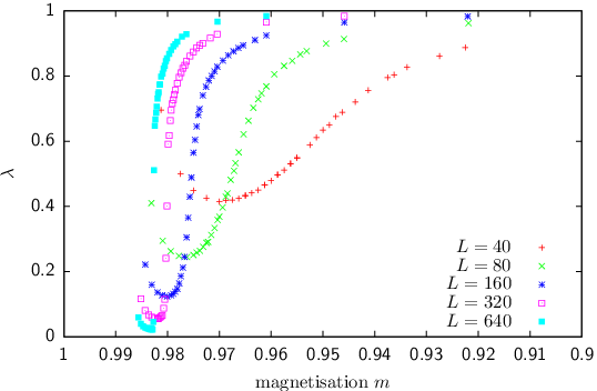
(b) 
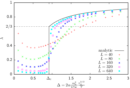

The increase of for can be explained by the fact that the minimal cluster size is and not an arbitrarily small fraction. In contrast, the excess that can be fixed analytically using Eq. (14) can be much smaller than .
In Fig. 17 we compare for of the three different models. The nice agreement of the data points is a clear indication for the lattice independent universal behavior of the theory. An explanation for the slight discrepancy between the n.n. and the triangular lattice on the one side and the n.n.n. model on the other might be given by the slightly different temperature ratio (see Table 1).

V Conclusion
Our Monte Carlo data clearly confirm the theoretical considerations of Biskup et al. Biskup et al. 2002; Biskup et al. 2003a for the case of the two-dimensional next-neighbour Ising system. While their results are only valid in the thermodynamic limit of large systems, we have shown that for practically accessible sizes the theory can also applied. The observed finite-size scaling behavior fits perfectly with their predictions for the infinite system.
Moreover we have demonstrated that the theory, which to date has only been proven for the square lattice nearest-neighbour case, is actually universal in the sense that it is independent of the underlying lattice. The Ising model on the two-dimensional triangular lattice and on the two-dimensional next-nearest neighour lattice both approach the theoretically expected results nicely. Apparently, for the same relative temperature the finite-size behavior is identical.
In order to achieve the correct scaling of the abscissa we presented several methods to estimate the Wulff free energy numerically. While in theory it should be straightforward to extract the value from the distribution of the magnetisation, due to limitations in the computer time for temperatures near the critical one, it can be more advantageous to resort to the isotropic approximation.
All simulations were performed in thermal equilibrium and the abundance of droplets of intermediate size could be confirmed visually by looking at the distribution of droplets. We only state this fact here, while a more detailed analysis and the corresponding graphs will be presented in a later publication together with more results on the finite-size scaling behavior of the systems and the shape of the free-energy barrier associated with the evaporation/condensation transition.
Acknowledgements.
We are indebted to Kurt Binder and Thomas Neuhaus for sharing their physical insight into the droplet nucleation mechanism, and wish to thank Roman Kotecký for helpful discussions on the formulation used in the present work. Work supported by the Deutsche Forschungsgemeinschaft (DFG) under grants No. JA483/22-1 and No. JA483/23-1 and in part by the EU RTN-Network ‘ENRAGE’: “Random Geometry and Random Matrices: From Quantum Gravity to Econophysics” under grant No. MRTN-CT-2004-005616. Supercomputer time at NIC Jülich under grant No. hlz10 is also greatfully acknowledged.References
- Fisher (1967) M. E. Fisher, Rep. Prog. Phys. 30, 615 (1967).
- Binder and Kalos (1980) K. Binder and M. H. Kalos, J. Stat. Phys. 22, 363 (1980).
- Furukawa and Binder (1982) H. Furukawa and K. Binder, Phys. Rev. A 26, 556 (1982).
- Neuhaus and Hager (2003) T. Neuhaus and J. S. Hager, J. Stat. Phys. 113, 47 (2003).
- Biskup et al. (2002) M. Biskup, L. Chayes, and R. Kotecký, Europhys. Lett. 60, 21 (2002).
- Biskup et al. (2003a) M. Biskup, L. Chayes, and R. Kotecký, Comm. Math. Phys. 242, 137 (2003a).
- Binder (2003) K. Binder, Physica A 319, 99 (2003).
- Virnau et al. (2004) P. Virnau, L. G. MacDowell, M. Müller, and K. Binder, in Computer Simulation Studies in Condensed Matter Physics XVI, edited by D. P. Landau, S. M. Lewis, and H.-B. Schüttler (Springer, Berlin, 2004).
- Nußbaumer et al. (2006) A. Nußbaumer, E. Bittner, T. Neuhaus, and W. Janke, Europhys. Lett. 75, 716 (2006).
- Biskup et al. (2003b) M. Biskup, L. Chayes, and R. Kotecký, J. Stat. Phys. 116, 175 (2003b).
- Lee et al. (1995) J. Lee, M. A. Novotny, and P. A. Rikvold, Phys. Rev. E 52, 356 (1995).
- Pleimling and Selke (2000) M. Pleimling and W. Selke, J. Phys. A: Math. Gen. 33, L199 (2000).
- Pleimling and Hüller (2001) M. Pleimling and A. Hüller, J. Stat. Phys. 104, 971 (2001).
- Wulff (1901) G. Wulff, Z. Kristallogr. Mineral. 34, 449 (1901).
- Zia and Avron (1982) R. K. P. Zia and J. E. Avron, Phys. Rev. B 25, 2042 (1982).
- Leung and Zia (1990) K. Leung and R. K. P. Zia, J. Phys. A: Math. Gen. 23, 4593 (1990).
- Kramers and Wannier (1941) H. A. Kramers and G. H. Wannier, Phys. Rev. 60, 252 (1941).
- Onsager (1949) L. Onsager, Nuovo Cim. (Suppl.) 6, 261 (1949).
- Yang (1952) C. N. Yang, Phys. Rev. 85, 808 (1952).
- Orrick et al. (2001) W. P. Orrick, B. G. Nickel, A. J. Guttmann, and J. H. H. Perk, Phys. Rev. Lett. 86, 4120 (2001).
- Fisher and Ferdinand (1967) M. E. Fisher and A. E. Ferdinand, Phys. Rev. Lett. 19, 169 (1967).
- Rottman and Wortis (1981) C. Rottman and M. Wortis, Phys. Rev. B 24, 6274 (1981).
- Baxter (1982) R. J. Baxter, Exactly Solved Models in Statistical Mechanics (Academic Press, London, 1982).
- Potts (1952) R. B. Potts, Phys. Rev. 88, 352 (1952).
- Sykes et al. (1973) M. F. Sykes, D. S. Gaunt, J. L. Martin, S. R. Mattingly, and J. W. Essam, J. Math. Phys. 14, 1071 (1973).
- Sykes et al. (1975) M. F. Sykes, M. G. Watts, and D. S. Gaunt, J. Phys. A: Math. Gen. 8, 1448 (1975).
- Shneidman and Zia (2001) V. A. Shneidman and R. K. P. Zia, Phys. Rev. B 63, 085410 (2001).
- Nightingale and Blöte (1982) M. P. Nightingale and H. W. J. Blöte, J. Phys. A: Math. Gen. 15, L33 (1982).
- Nußbaumer et al. (2007) A. Nußbaumer, E. Bittner, and W. Janke, Europhys. Lett. 78, 16004 (2007).
- Bürkner and Stauffer (1983) E. Bürkner and D. Stauffer, Z. Phys. B 53, 241 (1983).
- Hasenbusch and Pinn (1994) M. Hasenbusch and K. Pinn, Physica A 203, 189 (1994).
- Shlosman (1989) S. B. Shlosman, Comm. Math. Phys. 125, 81 (1989).
- Avron et al. (1982) J. E. Avron, H. van Beijeren, L. S. Schulman, and R. K. P. Zia, J. Phys. A: Math. Gen 15, L81 (1982).
- Onsager (1944) L. Onsager, Phys. Rev. 65, 117 (1944).
- McCoy and Wu (1973) B. M. McCoy and T. T. Wu, The Two-Dimensional Ising Model (Harvard University Press, Cambridge Mass., 1973).
- Janke (2003) W. Janke, in Computer Simulations of Surfaces and Interfaces, NATO Sci. Ser., II. Math., Phys. and Chem., edited by B. Dünweg, D. P. Landau, and A. I. Milchev (Kluwer, Dordrecht, 2003), vol. 114, pp. 111–135.
- Okabe et al. (1999) A. Okabe, B. Boots, K. Sugihara, and S. N. Chius, Spatial Tessellations: Concepts and Applications of Voronoi Diagrams (John Wiley & Sons, Chichester, 1999).
- Hoshen and Kopelman (1976) J. Hoshen and R. Kopelman, Phys. Rev. B 14, 3438 (1976).
- Agoston (2004) M. K. Agoston, Computer Graphics and Geometric Modelling (Springer, London, 2004).
- Heuer et al. (1997) A. Heuer, B. Dünweg, and A. M. Ferrenberg, Computer Physics Communications 103, 1 (1997).
- Janke (2002) W. Janke, in Quantum Simulations of Complex Many-Body Systems: From Theory to Algorithms, edited by J. Grotendorst, D. Marx, and A. Muramatsu (John von Neumann Institute for Computing, Jülich, 2002), vol. 10 of NIC Series, pp. 423–445.
- Earl and Deem (2005) D. J. Earl and M. W. Deem, Phys. Chem. Chem. Phys. 7, 3910 (2005).