Emergent fermions and anyons in the Kitaev model

The study of elementary excitations in strongly correlated systems is a fascinating field of current research. As exemplified in the fractional quantum Hall effect, such excitations can be very different from the elementary constituents present in the system. In the same spirit, emergent fermions and gauge fields in purely boson/spin systems have attracted much attention recently Wen 2004. The emergence of anyonic excitations in two-dimensional systems has also triggered a tremendous amount of interest, especially since its relevance for topological quantum computation (see Ref. S. Das Sarma, M. Freedman, C. Nayak, S. H. Simon, and A. Stern for a recent review) has been pointed out by Kitaev in a seminal paper Kitaev 2003 introducing the celebrated toric code.

More recently, Kitaev introduced a more realistic model Kitaev 2006 for which experiments using ultracold atoms or polar molecules have been proposed Duan et al. 2003; Micheli et al. 2006. This model is a two-dimensional spin-$1/2$ system on the honeycomb or brick-wall lattice, as illustrated in Fig. 1. It consists solely of Ising-like interactions but in different quantization axis. More precisely, the Hamiltonian reads

where $\sigma_{i}^{\alpha}$ are the usual Pauli matrices at site $i$. Without loss of generality Kitaev 2006, in the following, we assume $J_{\alpha}\geq 0$ for all $\alpha$ and $J_{z}\geq J_{x},J_{y}$.

Kitaev solved the model exactly by introducing Majorana fermions to represent the spin operators in an extended Hilbert space. In this way, the Hamiltonian is reduced to free fermions in a static $\mathbb{Z}_{2}$ gauge field on the honeycomb lattice. The physical states are selected by a projection step which simply amounts to a selection rule on the parity of the number of fermions Vidal et al., in agreement with the general conclusions of Ref. Levin and Wen 2003. The system exhibits a gapless phase for $J_{x}+J_{y}>J_{z}$, with non-Abelian anyonic excitations arising when a magnetic field is switched on Kitaev 2006. A contrario, for $J_{x}+J_{y}<J_{z}$, the system is gapped and the low-energy effective Hamiltonian, at lowest nontrivial order in perturbation ($J_{x},J_{y}\ll J_{z}$) and periodic boundary conditions, turns out to be exactly the toric code. Consequently, at this order, free Abelian anyons are present in the gapped phase.

Note also that an alternative treatment has been proposed Chen and Hu 2007; Chen and Nussinov 2008; Feng et al. 2007 based on the Jordan-Wigner transformation which transforms the spin system into a system of fermions with $p$-wave BCS pairing and a site-dependent chemical potential.

In this Letter, we focus on the gapped phase and we derive the low- and high-energy effective theory at high-order in perturbation. This allows us to show that i) the low-energy effective Hamiltonian is an extended toric code Hamiltonian with still static but interacting Abelian anyons ; ii) the high-energy excitations are free fermions, composed of a hardcore boson with an attached string of spin operators, hopping on a square lattice embedded in a magnetic field.

Our approach has some advantages which compensate for its perturbative nature and its restriction to the gapped phase. It provides a unified picture of the emergence of high- and low-energy excitations without introducing fermionic fields by hand as is done with Majorana or Jordan-Wigner fermionization. In addition, we work, from the beginning, in the thermodynamical limit, and derive analytical results for non-translational-invariant low-energy states.

Let us consider the model in the limit $J_{x},J_{y}\ll J_{z}$. In the limiting case $J_{x}=J_{y}=0$ the model is a collection of isolated $z$-dimers. Each dimer has four possible configurations : two low-energy states $\{|\!\uparrow\uparrow\rangle,|\!\downarrow\downarrow\rangle\}$ with energy $-J_{z}$ and two high-energy states $\{|\!\uparrow\downarrow\rangle,|\!\downarrow\uparrow\rangle\}$ with energy $J_{z}$. It is thus natural to interpret the change from a ferromagnetic to an antiferromagnetic dimer configuration as the creation of a particle, with an energy cost that we set equal to $1$ by chosing $J_{z}=1/2$. By construction, these particles are hardcore bosons hopping on the sites of an effective square lattice (see Fig. 1), together with an effective spin-$1/2$ indicating which kind of (anti-)ferro dimer configuration is realized. Among the four possible mappings we choose the following

where the left (right) spin is the one of the black (white) site of the dimer, and double arrows represent the state of the effective spin. Let us denote by $b^{\dagger}_{\boldsymbol{i}}$ ($b^{\phantom{\dagger}}_{\boldsymbol{i}}$) the creation (annihilation) operator of a hardcore boson at site ${\boldsymbol{i}}$ (bold letters denote effective sites), and $\tau_{\boldsymbol{i}}^{\alpha}$ the Pauli matrices of the effective spin at the same site. With these notations, the number of bosons in the system is $Q=\sum_{\boldsymbol{i}}b^{\dagger}_{\boldsymbol{i}}b^{\phantom{\dagger}}_{\boldsymbol{i}}$ and the Hamiltonian (1) can be rewritten as Vidal et al.

where $N$ is the number of $z$-dimers,

with hopping and pair creation operators

The vectors ${\boldsymbol{n}}_{1}$ and ${\boldsymbol{n}}_{2}$ are shown in Fig. 1b. Let us underline that $[W_{p},t_{\boldsymbol{i}}^{{\boldsymbol{j}}}]=[W_{p},v_{\boldsymbol{i}}^{{\boldsymbol{j}}}]=0$ for all $(p,{\boldsymbol{i}},{\boldsymbol{j}})$ where the conserved plaquette operators Kitaev 2006 read (with notations given in Fig. 1)

At this stage, note that both the mapping (2) and the form of the Hamiltonian (3) are simply an alternative description of the problem which is always valid, even in a nonperturbative regime. The main difficulty resides in the fact that, now, one has to deal with hardcore bosons coupled to effective spin degrees of freedom. Of course, one could use a fermionization trick and solve the model directly as done by Kitaev Kitaev 2006. However, the procedure used in the following can be applied to nonexactly solvable models and further allows, in the present case, for a clear identification of the excitations.

In general, a Hamiltonian of the form (3) cannot be diagonalized exactly. Here, following Kitaev, we choose to treat it perturbatively in the limit $J_{x},J_{y}\ll J_{z}$. Nevertheless, the Green’s functions method used in Ref. Kitaev 2006 turns out to be rather hard to implement at high order and/or high energy. Instead, we use an alternative approach based on continuous unitary transformations (CUTs) Wegner 1994 whose perturbative version Stein 1997; Knetter and Uhrig 2000 is especially well-suited to the problem at hand. Technical details will be given in a forthcoming publication Vidal et al..

The main idea is to transform the Hamiltonian (3) which does not conserve the number of bosons into an effective Hamiltonian $H_{\mathrm{eff}}$ which satifies $[H_{\mathrm{eff}},Q]=0$. As explained in Ref. Knetter et al. 2003, $H_{\mathrm{eff}}$ is a sum of $k$-quasi-particle (QP) operators with $k\in\mathbb{N}$. The $k=0,1$ contributions can be written as

Here $\{p_{1},p_{2},\ldots,p_{n}\}$ denotes a set of $n$ plaquettes and the sum, $\{{\boldsymbol{j}}_{1},\ldots,{\boldsymbol{j}}_{n}\}$ represents a sequence of $n$ connected sites. The perturbative aspect comes from the fact that the coefficients appearing in $H_{\mathrm{eff}}$ are obtained as series expansions in $J_{x}$ and $J_{y}$. We have computed the 0-QP amplitudes $E_{0}$ and $C_{p_{1},\ldots,p_{n}}$ up to order 10 and the 1-QP amplitudes $\mu$ and $D_{{\boldsymbol{j}}_{1},\ldots,{\boldsymbol{j}}_{n}}$ up to order 4. These expressions, being quite lengthy, will be given in a longer paper Vidal et al., as well as a discussion of ($k\geqslant 2$)-QP sectors.

Let us first discuss the low-energy physics, i.e. the spectrum of $H_{\mathrm{eff}}^{0\,\mathrm{qp}}$. The most striking result is that the latter is only expressed in terms of the conserved quantities $W_{p}|_{0\,\mathrm{qp}}=\tau_{\mbox{\tiny L}}^{y}\,\tau_{\mbox{\tiny U}}^{z}\,\tau_{\mbox{\tiny R}}^{y}\,\tau_{\mbox{\tiny D}}^{z}$. Thus, for any (vortex) configuration of the $W_{p}$’s which can take two values $\pm 1$, one readily gets the ground state energy of the corresponding sector. We wish to emphasize that at order 4 (lowest nontrivial order), as already discussed by Kitaev Kitaev 2006, the only nonvanishing contribution (apart from $E_{0}$) involves only single plaquette-terms and one recovers the toric code Hamiltonian with its Abelian anyons Kitaev 2003. At order 6, one gets the following corrections to these terms

but, more interestingly, one also has some two-plaquette terms :

Actually, when increasing the perturbation theory order, one generates higher and higher multi-plaquette terms. Thus, the low-energy effective theory of the Kitaev model turns out to be an interacting anyon theory whose eigenstates are those of the toric code. The single-vortex energy and the two vortices interaction energies of three configurations are given in Fig. 2 at order 10, for $J_{x}=J_{y}=J$.

It should finally be noticed that although the vortices interact, they remain static since $W_{p}$’s are conserved quantities.

In each sector defined by a configuration of the $W_{p}$’s, we shall now see that the excitation spectrum is of fermionic nature. As proposed by Levin and Wen Levin and Wen 2003, the statistics can be directly determined from the hopping operators algebra. Let us consider the exchange process depicted in Fig. 3. The corresponding operator sequence is :

or, equivalently, $t^{{\boldsymbol{i}}}_{{\boldsymbol{j}}}t^{{\boldsymbol{k}}}_{{\boldsymbol{i}}}t^{{\boldsymbol{i}}}_{{\boldsymbol{l}}}=-t^{{\boldsymbol{i}}}_{{\boldsymbol{l}}}t^{{\boldsymbol{k}}}_{{\boldsymbol{i}}}t^{{\boldsymbol{i}}}_{{\boldsymbol{j}}}$. This latter identity shows that the quasi-particles made of a hardcore boson and an effective spin-1/2 obey fermionic statistics.

We shall now see that solving the excitation spectrum is completely equivalent to solving a problem of free fermions in a magnetic field on the square lattice. Therefore, let us focus on the first-order perturbation theory for which $H_{\mathrm{eff}}^{1\,\mathrm{qp}}=Q+T_{0}$ and consider a single quasi-particle. Then, one can easily see that the momenta $\big(H_{\mathrm{eff}}^{1\,\mathrm{qp}}-1\big)^{m}$ for all $m$ are strictly equal to those of a pure hopping fermion Hamiltonian in a magnetic field provided the magnetic flux per plaquette mimicks the configuration of the $W_{p}$’s. This is easily seen by noting that the product of the hopping operator around a plaquette $p$ is given by $t^{\boldsymbol{i}}_{\boldsymbol{l}}t^{\boldsymbol{l}}_{\boldsymbol{k}}t^{\boldsymbol{k}}_{\boldsymbol{j}}t^{\boldsymbol{j}}_{\boldsymbol{i}}=W_{p}$, with $\{{\boldsymbol{i}},{\boldsymbol{j}},{\boldsymbol{k}},{\boldsymbol{l}}\}$ being any sequence of connected sites chosen among L, U, R and D (see Fig. 1).

The $W_{p}$’s being conserved quantities, from a purely spectral point of view one can replace the Pauli matrices in the hopping operators by pure numbers $\pm 1$ constraining the fluxes per plaquette (in unit of the flux quantum) to be $\phi_{p}=0$ for $W_{p}=+1$ or $\phi_{p}=1/2$ for $W_{p}=-1$. At higher order, this mapping remains true (with hoppings from one site to any other site) but one needs to go beyond this simple argument to prove the correspondence between both spectra Vidal et al.. Let us simply mention that this is done by building a basis of the 1-QP subspace, which turns out to be made of states with one string of spin flips attached to one hard-core boson (yielding a fermion), as can be inferred from the form (6) of the hopping operators, and illustrated in Fig. 4. Note that the string fluctuates, as in the construction of anyons in Kitaev 2003.

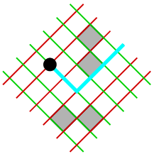
To illustrate the mapping, let us consider the 1-QP vortex free state ($W_{p}=+1,\forall p$). The spectrum of $H_{\mathrm{eff}}^{1\,\mathrm{qp}}$ is made of a single band whose dispersion relation is given, at second order, by :

where the wave vector $(k_{x},k_{y})\in[-\pi,\pi]\times[-\pi,\pi]$. The gap in this sector is then obtained by minimizing $E_{\rm free}$ and one gets $\Delta_{\rm free}=1-2(J_{x}+J_{y})$. Note that, in this case, the perturbative result at order 1 coincides with the nonperturbative result obtained by Kitaev Kitaev 2006 and one recovers the transition point at $J_{x}+J_{y}=1/2=J_{z}$.

Let us complete our analysis with a comparison to the Majorana (or Jordan-Wigner) fermion formalism. In the latter, one can compute the full spectrum exactly, by diagonalizing, for each configuration of the $W_{p}$’s with $2N$ spins, a $2N\times 2N$ matrix. Within our approach, we have a $N\times N$ matrix to consider. Although we have seen that analytical (perturbative) results can be obtained for $H_{\mathrm{eff}}^{0\,\mathrm{qp}}$, even for non-translational-invariant $W_{p}$’s, for $H_{\mathrm{eff}}^{1\,\mathrm{qp}}$ the problem is thus essentially as complicated as in the Majorana (or Jordan-Wigner) fermion formalism. In this case, the main interest of our method is thus to give a physical picture of the high-energy excitations as emerging fermions.

Furthermore, the continuous unitary transformations allow for the calculation of correlation functions. In the 0-QP subspace, as we show below, some of these can again be expressed as a series in $W_{p}$ operators, as was the case for the eigenvalues of $H_{\mathrm{eff}}^{0\,\mathrm{qp}}$. Here, we focus on the correlation function $C^{zz}_{\boldsymbol{i}}=\langle\sigma^{z}_{{\boldsymbol{i}},\bullet}\sigma^{z}_{{\boldsymbol{i}},\circ}\rangle$ where ${\boldsymbol{i}},\bullet$ and ${\boldsymbol{i}},\circ$ are the black and white sites of a given $z$-dimer ${\boldsymbol{i}}$ (see Fig. 1). Such a correlation function can be computed exactly for a translationnaly invariant configuration of $W_{p}$’s, either by using the technique developped in Baskaran et al. 2007 or, in a much simpler way, thanks to the Hellman-Feynman theorem Vidal et al.. However, none of these two methods can be used effciently for a non-translational-invariant configuration of the $W_{p}$’s.

As a first step, one has to translate $C^{zz}_{\boldsymbol{i}}$ into the effective spin and boson degrees of freedom, which yields $C^{zz}_{\boldsymbol{i}}=\langle(-1)^{b^{\dagger}_{\boldsymbol{i}}b^{\phantom{\dagger}}_{\boldsymbol{i}}}\rangle$. Then, the observable appearing in the angular brackets has to be transformed with the same unitary transformation as the one applied to the Hamiltonian Vidal et al.; Knetter et al. 2003. As an illustration, we give the result in Fig. 5 at order 4 which is the lowest nontrivial order where the $W_{p}$’s appear in the expansion. Note that we have used the same notation $W$ for the operator and its expectation value on a 0-QP state. This result shows how the correlation function is modified by the presence of surrounding anyons. Of course, at higher order, anyons further apart would also contribute Vidal et al. as was already the case for the spectrum of $H_{\mathrm{eff}}^{0\,\mathrm{qp}}$.

To conclude, we wish to emphasize that the method we have used here, based on a perturbative approach of the CUTs, can be applied to nonexactly solvable models as well. In addition, as we have shown, it is especially efficient to compute the spectrum but also the expectation value of observables, even at high order in perturbation. Thus, we strongly hope that it constitutes a powerful tool to investigate, for instance, the non-Abelian anyons recently proposed by Yao and Kivelson for a time-reversal symmetry breaking version of the Kitaev model Yao and Kivelson 2007; Vidal et al..