Moduli Evolution in the Presence of Matter Fields and Flux Compactification
Abstract:
We provide a detailed analysis of the dynamics of moduli fields in the KKLT scenario coupled to a Polonyi field, which plays the role of a hidden matter sector field. It was previously shown that such matter fields can uplift AdS vacua to Minkowski or de Sitter vacua. Additionally, we take a background fluid into account (which can be either matter or radiation), which aids moduli stabilisation. Our analysis shows that the presence of the matter field further aids stabilisation, due to a new scaling regime. We study the system both analytically and numerically.
Keywords:
physics of the early universe, string theory and cosmology, cosmological applications of theories with extra dimensions1 Introduction
Theories beyond the standard model, such as string theory, predict the existence of massless (or nearly massless) scalar fields. These so-called moduli fields may contain, for example, the information about the dynamics of extra spatial dimensions, or, as it is the case of the string theory dilaton, they determine the coupling strength of gauge fields. In addition, these fields usually interact, with gravitational strength, to other particles, thereby mediating a new (“fifth”) force. Since so far we have neither observed any significant time-dependence of gauge couplings nor detected new forces, the moduli fields have to be stabilised [1]. This should happen at some stage during the cosmological evolution, which is one of the problems addressed in string cosmology. It was emphasized in [2] that stabilising the string theory dilaton in a cosmological framework is a rather difficult, because of the the small barrier height separating a local Minkowski (or de Sitter) vacuum and the steepness of the potential. The situation can be improved if background fluids (either radiation or matter) or temperature dependent corrections are taken into account (for work in this direction see e.g. [3, 4, 5, 6]).
In order to stabilise the moduli fields, a mechanism is required which gives them a mass. Additionally, the resulting vacuum energy should be very small and non-negative and the vacuum itself quasi-stable (i.e. with a life-time much longer than the age of the universe). Recently, compactification mechanisms with fluxes on internal manifolds have been extensively studied (see [7], a review can be found in [8]); a well-investigated scenario is the KKLT proposal [9]. Within this latter setup, moduli fields are stabilised and the resulting cosmological constant can be fine-tuned to be either zero or very small. To obtain a realistic scenario, a crucial ingredient in these mechanisms is a “lifting” procedure, which raised a supersymmetric AdS-vacuum to become a Minkowski or even a (quasi) de-Sitter vacuum. In the original KKLT proposal, an anti-D3 brane was added, explicitly breaking supersymmetry. In an alternative proposal, D-terms were considered to up-lift the AdS-vacuum, which requires the existence of charged matter fields [10, 11, 12].
Recently it was pointed out that interactions of the moduli fields with a hidden matter sector can also result in an effective uplifting to Minkowski or de Sitter vacua. The idea of this procedure is to take matter fields into account (such fields will be present in any realistic theory). The resulting interaction terms in the scalar potential lead to spontaneous supersymmetry breaking, with local minima which have a small and positive vacuum energy density. This procedure is known as F-term uplifting (for recent work, see see e.g. [13, 14, 15, 16, 17, 18, 19, 20] and references therein). An appealing feature is that this procedure can result in a small gravitino mass, while maintaining a high potential barrier, resulting in long-lived de-Sitter vacua [14, 17, 18, 21].
In this paper, we investigate the cosmological dynamics of the moduli fields and matter fields in the the context of F-term uplifing. As a toy model, we will couple the KKLT model with the Polonyi model [22], following [14, 20, 21, 23]. This model is simple enough to study the dynamical consequences of the interactions between the moduli fields and matter fields, but we believe that our results can be generalised to more complex models. In particular we are interested in whether the interaction will facilitate or impede the stabilisation of the moduli fields in the cosmological context. The paper is organized as follows: In Section 2 we formalise the set-up and write down the essential equations. In Section 3, we discuss the properties of the potential. We review past results, in the context of our potential, in Section 4 and generalise to multi-field scenarios in Section 5 (two real fields). The full dynamics for two complex fields is presented in Section 6. We briefly consider the effects of a radiation background fluid in Section 7. We conclude in Section 8. We give further useful formulae in the Appendices and derive the new scaling regime.
2 Background Equations
We begin by stating the four-dimensional SUGRA action, which is of the form
| (1) |
where is the Kähler metric, are complex chiral superfields and is the scalar potential. is the 4-dimensional Newton constant,
| (2) |
The effective scalar potential is given, with given Kähler metric and superpotential , as
| (3) |
where is the inverse Kähler metric and .
The following equations of motion for the real and imaginary parts of superfields are [26]
| (4) |
where refers to the real (imaginary) part of the scalar fields and () are used to denote the derivative of the potential with respect to the real (imaginary) parts of the fields, respectively. The connections on the Kähler manifold are given by
| (5) |
There are two different sectors in the model considered here; one involves a modulus field , whereas the other sector contains a matter field . Both fields will be taken as complex fields. The corresponding Kähler potential [21], which arises in type IIB and heterotic string theory, is
| (6) |
Following [21, 23], for example, we consider the combination of the KKLT [9] and the Polonyi model, for which the superpotential is given by
| (7) |
so that the resulting scalar potential is given by
| (8) |
The differential equations describing the dynamics of the field are given by
| (9) |
where we write . Furthermore, we consider a background fluid with density and with equation of state . Energy conservation dictates that
| (10) |
We consider to be a complex field, , so that the equations of motion can be written as
| (11) |
The Friedmann equation reads
| (12) |
Since is not a canonical field, it is convenient to define a new field
| (13) |
Additionally, the equations for the fields are easier to solve if we define a new set of variables as follows
| (14) |
and
| (15) |
With these variables, the Friedmann equation becomes
| (16) |
where . The evolution of Hubble parameter is
| (17) |
where the prime denotes differentiation with repect to -fold number , defined by
| (18) |
The equations of motion for the fields are now given by
| (19) | |||||
and
| (20) |
In these equations, we have defined and to be
| (21) |
| (22) |
For the remainder of this paper, we solve the above equations, in order to investigate the stabilisation of the moduli fields, and , in the presence of the matter fields, and , and the background fluid, .
3 Properties of the Potential
As a specific example in this paper, following [21], we take the potential parameters to be
| (23) |
Additionally, is assumed to be real and is fine-tuned such that the potential is zero (or the cosmological constant ) at the local minimum. For the values above, the local minimum is found at the co-ordinates
| (24) |
 |
 |
 |
 |
In Figs. 1 and 2 we show the shape of this potential with the parameters given above. Since there are four independent fields, we fix two fields at their local minimum values and plot the remaining two fields. For convenience, we plot the canonical field, , instead of . In Fig. 1 the local minimum of this model is seen, where is stabilised at . As , the potential vanishes. Along the direction, the potential increases as departs from the minimum. As can be seen, the minimum of depends directly on the value of . Around the local minimum, . For , the potential can be approximated by
| (25) |
with , where the minimum of is . Note that the direction is much steeper than along the direction. On the left hand side of Fig. 2, we show the sinusoidal shape of , with periodicity of , with one minimum at zero. On the right hand side, the minimum of is seen to exist at zero and shows symmetry about because we assume in the figure. The values of and (defined in Eqns. (21-22)) over useful ranges are plotted in Fig. 3.
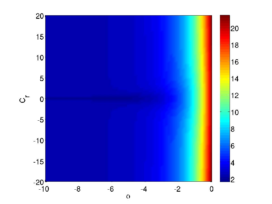

It should be noted that, as the and evolve away from their minima, the shape of the potential changes from that shown in the figures. This will become important when we consider the evolution of the imaginary parts of the fields, and .
4 Review of Single Field Dynamics
We begin by reviewing known results [4, 25] and consider only real fields; we put the imaginary fields in the minimum point, , so that these fields do not evolve. This will enable isolation of the effects of each field (real and imaginary parts). Some of the results obtained will prove vital later.
In this simplifed scenario, the potential becomes
| (26) |
Further, to compare to single field dynamics, for negatively large , we set in its local minimum () initially, such that it does not evolve until the final stages of the evolution. Even with only evolving, due to the background fluid and the potential, the dynamics are non trivial.


In this section, we will closely follow [26] and will refer to an example trajectory shown in Fig. 4. We assume that starts with zero kinetic energy from a point (this terminology will become useful later) and is close to unity initially (). As the field starts to evolve, as long as is small enough, the potential energy quickly dominates the dynamics, seen in Region 1 of Fig. 4. As the potential becomes more steep ( increases sharply around for our potential), the evolution becomes kinetically dominated, called ”kination” shown in Region 2. Once the background fluid dominates, the field is effectively frozen at a point (in Region 3), and the field only starts rolling again once this fluid has sufficiently diluted.
As the field recommences to roll, one of two things can happen; either the scalar field dominates again (Region 1) or a scaling regime is found, in which the potential and kinetic energies track the background fluid (Region 4), which occurs for our trajectory. The choice of regime is specified by a scaling condition:
| (27) |
where we restate that . For our choice of potential, this condition is always satisfied when with a matter background fluid. The scaling regime ends when this condition is subsequently violated, which occurs if the potential flattens, for example near the minimum. If , the end of scaling occurs near the minimum and the field stabilises. If but smaller than the local maximum value, the field will still stabilise. Conversely, if is larger than the local maximum value, the field will roll to infinity. In our case, the fields are stabilised.
In the following, we state the analytical solutions for the single field scenario. In particular, two initial branches can be distinguished; and (the latter being described heuristically above). It is convenient to consider the new variables, , etc. (defined earlier) for analysis of the evolution.
4.1
When , following [24], the initial evolution is given by
| (28) |
where we assume , for which the solution is
| (29) | |||||
| (30) |
This solution is valid until is no longer insignificant (), at which point, the kinetic energy starts to dominate, and kination starts. Due to the non-constancy of , no approximation can be found for this period. However, during this stage, due to the insignificance of , increases to almost unity, as the kinetic energy fully dominates the evolution. Due to the expansion of the universe, the kinetic energy is diluted and slowly the background fluid becomes significant (, ), at which point the field becomes frozen at .
When the potential is insignificant, the system during kination is greatly simplified and can be described by [4]:
| (31) |
If starts at a value , the solution is
| (32) |
During this decay, the field moves a distance, , given by
| (33) |
after which the field freezes at . (Note that is never exactly unity since ).
4.2
When , the the kinetic energy of never fully dominates, in that , before the background fluid takes over. As seen in Fig. 4, the background fluid is never totally negligible, which complicates the evolution. However, kination starts when starts to increase (, ). Once is negligible, moves a further distance given by Eqn (33) before freezing at . Although this regime cannot be solved analytically, one point can be made: in this case, the field freezes earlier (due to less kinetic energy overall, ), so that is smaller than that when .
Numerically, we find that, for and (an example that will prove useful later), stabilisation only occurs when and . We define these points as and .
5 Two Real Fields with a Matter Background Fluid
This section extends the previous single field scenario, by considering the evolution of an additional scalar field. Specifically, we consider the evolution of , in which direction the potential is much steeper than the -field previously considered. We will show that this leads to a new mechanism for stabilisation, due to the presence of a new scaling regime.
We will explain the dynamics using several representative trajectories for which shown in Fig. 5:
- I
[solid line (blue)]
- II
[dotted line (red)]
- III
[dashed line (green)]
- IV
[dotted line (magenta)]
We take (a background matter fluid) and consider two cases and . The initial velocities of the fields are zero.
Fig. 5 shows the evolution of the fields and against -folding number, , and the trajectories in the - plane. The evolution of each energy component for trajectories I and II are shown in Figs. 6 and 7. Trajectory III is identical to Trajectory II (although stabilisation does not occur) and is not shown. The evolution of the energy components for trajectory IV is shown in Figs. 8. Note that Fig. 6 strongly resembles Fig. 2 of [26].


As in the single field case, similar regimes can be identified: (1*) field domination, (2*) kination, (3*) freeze-out and (4*) scaling. The asterix (*) denotes two-field evolution, in order to separate it from the single field case. When approaches zero, however, these regimes are followed by a period of oscillation around (Region 5*), further followed by the regimes (1-4) of single field evolution (as in the previous section). After this, the field is either stabilised or rolls over. It should be noted that, due to the steepness in the direction (), the field arrives in its minimum quickly with the field still running toward the minimum. Due to this, the second half of the dynamics follows single field evolution, as was discussed in the previous section.


We will now derive some useful approximations for the first part of the evolution, when . Depending on the initial value of , there are two branches of evolution, A and B. These are shown as a flowchart in Fig. 9, which also shows the path of each example trajectory.

5.1 Branch A
Example trajectories for this branch are seen in Fig. 6 and 7, where . Initially, for a very brief time, the potential energy dominates but since the solution of field domination is not stable (see Appendix C) this energy is quickly transfered to the kinetic energy of both fields, and . This change of energy can be described by
| (34) |
for which the solutions are given by
| (35) |
This is the extended solution of Eqns. (29) and (30) for two fields. The maxima of these solutions, which can be considered to define the start of kination, are approximately given by
| (36) |
Here we have neglected the evolution of , but the error induced should be small. We shall use the notation that a subscripted bracket will denote the end of the regime of interest, here kination (Region 2*), but we omit the asterix for brevity.
During kination, we may assume and the the solution is
| (37) |
When the potential energy negligible compared to the kinetic energy, from the Klein-Gordon equation
| (38) |
for which the solution is . Therefore the kinetic energy is proportional to . This is the same for the field.
Alternatively, in this region, we can obtain
| (39) |
where we have used the original definition of and for the third term. This gives a direct relation between and
| (40) |
where we have used the initial values of kination from Eqn. (36). The freeze-out point can be calculated by integrating these solutions
| (41) |
where and Note however, that when the initial background density is small enough, the transfer of potential energy to kinetic energy is so quick that we can consider starting at a point , with kinetic energies given by ,.
5.2 Branch B
An typical trajectory of this branch is shown in Fig. 8. If is initially large, then the potential energy can never dominate and kination is not achieved. Instead, the equation of motion for the background fluid is given by
| (42) |
As potential energy is converted to kinetic energy, becomes negligible in a few e-folds and we quickly obtain the solution
| (43) |
Though the fields obtain some kinetic energy from the potential energy, it is suppressed compared to the background density. Quickly, and the fields become frozen. This process is very fast and we can make the approximation and
5.3 Scaling
We calculate the full scaling solution and condition in Appendix B. We will use the main results in this section. The two-field scaling condition is given by
| (44) |
At the freeze-out point, if the condition for scaling is satisfied, then the fields track the background fluid. We define
| (45) |
Making the assumption that
| (46) |
which is reasonable in the ranges and for our potential, we obtain
| (47) |
where
| (48) |
This is a valid solution only when . When , however, changes form and begins to decrease (and later increases again). This deviation from leads to an increase in (as seen around in Fig. 6). Scaling proceeds until goes to around , where the scaling condition is violated.
During scaling, the background fluid density takes the form
| (49) |
and the trajectory is specified by
| (50) |
From Fig. 3, we may take approximately constant and from Eqn. (26)
| (51) |
so that
| (52) |
At the end of the scaling regime, as found numerically, the fractional energy of a matter background fluid is
| (53) |
and the kinetic energy of is small. We find that this fractional background density is numerically independent of the initial values of the dynamics and is determined only by the existence of scaling solution (i.e. potential dependent). Additionally, from Eqn. (52), when the trajectory reaches , we find
| (54) |
where either [,] are calculated from Eqn. (41) (Branch A) or [,] (Branch B). For a matter background and , trajectories always scale. When , only trajectories with have time to enter a scaling regime. This region is depicted by regions (i) in Fig. 5 and separated with a dotted line.
5.4 Oscillation
If the trajectory undergoes scaling, then it is clear from Eqn. (47) that, for our potential at least, and there is more kinetic energy in than in . When the trajectory reaches the minimum (), the trajectory oscillates but is almost constant; it acts as if it is almost frozen at a point with .
If the trajectory does not scale (like Trajectories II and III), the trajectory gently oscillates around the minimum, with not fixed. Due to the relative gradients, and , the kinetic energy is shared between the fields, but the expansion of the universe acts to damp the oscillations. Finally, the background fluid dominates and the fields stop rolling at a point . At this point, we find numerically that once again.
After freeze-out, and the trajectory enters single field dynamics as discussed in Section 4.
5.5 Stabilisation Regions
We shall characterise a stabilising trajectory by the initial conditions for and which lead to final stabilisation. Samples of the stabilisation regions for two real fields can be seen in Fig. 5. Greyed out regions denote initial field values for trajectories which do not result in stabilisation. We will see that the important factor in stabilisation is the point , the value at which the - field freezes on the line, after either scaling or oscillation.
5.5.1
We will first explain the stabilisation region for a large background fluid density, such as when as shown in Fig. 5. A trajectory starting at large will follow similar dynamics as Trajectory IV. After freezing at a point [,], the fields will quickly reach a scaling regime. When , scaling ends and the -field oscillates around the “valley” and is effectively fixed at . Henceforth, the trajectory follows single field dynamics, with initial conditions and .
As discussed in Section 4, stabilisation depends merely on these initial conditions. Stabilisation may occur only when for , as is seen in Fig. 5. The slight asymmetry of the stabilisation region (seen for large ) is due to the asymmetry of the potential; the local minimum does not occur at . Trajectories which start close to the minimum are easier to stabilise.
We have numerically simulated trajectories only within . Note however, that all trajectories with within the stabilisation bounds at will lead to stabilisation. Therefore the allowed region extends to , due to the scaling solution.
5.5.2
The stabilisation region for looks vastly different from the previous example, as can be seen in Fig. 5. However, the underlying structure is the same. In regions (i), similar constraints are seen. These are due to scaling solutions, which result in the -field freezing on the axis between as before.
In region (ii), however, though the scaling condition is satisfied, the field does not have enough time to reach this scaling regime before reaching . Thus the field has enough kinetic energy at the crossing point to oscillate around (seen in Fig. 5). As described earlier, the trajectory settles into the minimum at at a point . As long as is within the range , the trajectory will lead to stabilisation. Therefore Trajectory II stabilises () whilst Trajectory III does not ().
The conical boundary of region (ii) depends on the energy density of the background fluid. For smaller , the kinetic energies are less damped and oscillate more widely. Since the field gains more kinetic energy initially (from potential energy) and is less damped, the fields travel further before settling at a point . Therefore as decreases, the conical bound moves left and the stabilisation area increases.
The asymmetry seen between regions (iii) and (iv) is once more again to the asymmetry of the potential; trajectories starting in region (iii) are pushed towards the minimum (due to the gradient) and stabilise, whereas trajectories from region (iv) are pushed away from the minimum.
6 Dynamics of Complex Fields
In this section, we include the dynamics of the imaginary parts of the fields, and , in order to fully generalise our model. The existence of non zero imaginary parts changes the shape of the potential in the - plane during evolution. As an example we consider a trajectory with initial values:
| (55) |
The evolution of the fields for this trajectory are shown in Fig. 10. It can be seen that, even though , this field is given a “kick” since
 |
 |
 |
 |
We show the evolution of each energy component in Fig. 11, where the kinetic energy of is seen to be negligible. This is due to the fact that and is not generic.


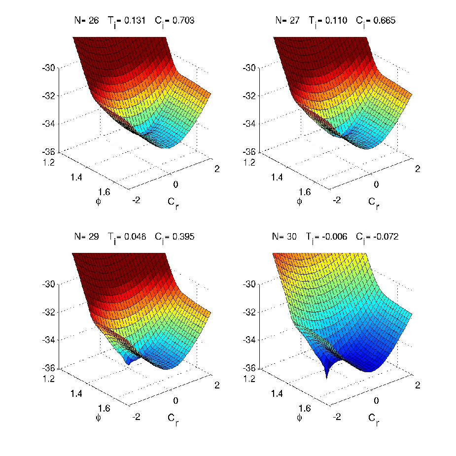
In Fig. 12 we show the contour plots of the potential in the plane for the above trajectory at e-folding numbers . In the top lefthand plot, where and , the local minimum almost disappears. However, at larger N and smaller , the potential changes shape and finally around the local minimum re-appears and the fields find this minimum. Thus we see that evolution of the imaginary fields can change the possibility of stabilisation. In fact, the evolution of the potential works to push the fields into the local minimum; as the fields get close to the position of the local minimum, the potential barrier effectively increases (the plateau is raised) and the fields are pushed back towards the re-emerging minimum.
In order to understand the full stabilisation region, a coarse 4-dimesional grid of trajectories was analysed numerically, in which each point represents the initial conditions for [,,,]. Three such grids were run, for . The results are shown in Fig. 13 for the 3-D volume --. We do not show the direction, since all values lead to identical surface plots (this is due to the symmetry seen in Fig. 2).
 |
 |
 |
 |
 |
 |
It is convenient to define a measure of goodness of stability. Firstly, to determine whether the background fluid adds stabilisation, we define an overall normalised, 4-D volume, , which is given by the volume of stabilised trajectories as a percentage of the total volume. In addition, we may calculate the ratio of stabilised trajectories to the total trajectories on a given 2-D plane (again, as a percentage), , where and denote the fixed values of the remaining fields. (For example represents the stabilisation area of the - plane when and ).
The numerical results for the measure of goodness are given in Tables 1 and 2. It should be well noted that the numbers quoted are intended to show a trend and are only indicative. Numerically, we rely on a finite volume, with finite (coarse) spacing. We chose a grid size that was numerically feasible within timescales. The may preclude us from resolving all the fine structure. We do note, however, that the fine structure arises from the asymmetry of the potential and the fine-tuning of the trajectories. This will be more relevant when we consider a radiation background fluid.
| Matter | Radiation | ||
|---|---|---|---|
| (%) | (%) | ||
| Matter | Radiation | |
| (%) | (%) | |
Our results indicate that a background matter fluid aids stabilisation, consistent with previous work [4, 25, 26]. In addition, the presence of matter fields further aids stabilisation. Importantly, while a non-zero value of assists the stabilisation of , the imaginary part further increases the stabilsation regions.
7 Radiation ()
For completeness, we briefly consider the effects of a radiation background fluid, in place of a matter fluid. All the equations in the preceding sections are valid, where . The results are shown in the righthand column of Fig. 13 and Tables 1 and 2. The main conclusions are:
- 1.
For all scenarios, the stabilisation region is much reduced, compared to when .
- 2.
Increasing again aids stabilisation.
- 3.
Due to the reduced cosmological friction acting on the fields, more fine-tuning is necessary for trajectories to find the local minimum.
- 4.
We observe the same trend of stabilisation when and are non-zero as for the matter background fluid, although the effects are less pronounced.
8 Conclusion
In this paper, we have considered moduli stabilisation in the KKLT scenario coupled to a Polonyi matter field, a model which has been previously studied in the context of particle phenomenology. In this scenario, the AdS vacuum is uplifted by F-terms in supergravity. We have examined the evolution of two complex fields (one modulus and one matter field), taking also a background fluid into account, either matter or radiation. We find that the presence of both the background fluid and the matter field enlarge the region leading to stabilisation of the moduli fields, due to a new scaling regime. Although a more detailed treatment is necessary, we believe that our conclusions will hold for similar scenarios, where the new direction is steep. A matter background fluid aids stabilisation more than radiation, consistent with previous studies.
Acknowledgments.
The authors acknowlege the use of the package “SuperCosmology” to calculate the scalar potential [27] and would like to thank STFC for financial support.References
- [1] M. Dine and N. Seiberg, “Is The Superstring Weakly Coupled?,” Phys. Lett. B 162 (1985) 299.
- [2] R. Brustein and P. J. Steinhardt, “Challenges for superstring cosmology,”, Phys. Lett. B 302 (1993) 196 [arXiv:hep-th/9212049].
- [3] N. Kaloper and K. A. Olive, “Dilatons in string cosmology,” Astropart. Phys. 1 (1993) 185.
- [4] T. Barreiro, B. de Carlos and E. J. Copeland, “Stabilizing the dilaton in superstring cosmology,” Phys. Rev. D 58 (1998) 083513 hep-th/9805005.
- [5] T. Barreiro, B. de Carlos and N. J. Nunes, “Moduli evolution in heterotic scenarios,” Phys. Lett. B 497 (2001) 136 [arXiv:hep-ph/0010102].
- [6] G. Huey, P. J. Steinhardt, B. A. Ovrut and D. Waldram, “A cosmological mechanism for stabilizing moduli,” Phys. Lett. B 476, 379 (2000) [arXiv:hep-th/0001112].
- [7] S. B. Giddings, S. Kachru and J. Polchinski, “Hierarchies from fluxes in string compactifications,” Phys. Rev. D 66 (2002) 106006 [arXiv:hep-th/0105097].
- [8] M. R. Douglas and S. Kachru, “Flux compactification,” Rev. Mod. Phys. 79 (2007) 733 [arXiv:hep-th/0610102].
- [9] S. Kachru, R. Kallosh, A. Linde and S. P. Trivedi, “De Sitter vacua in string theory,” Phys. Rev. D 68 (2003) 046005 hep-th/0301240.
- [10] C. P. Burgess, R. Kallosh and F. Quevedo, “de Sitter string vacua from supersymmetric D-terms,” JHEP 0310 (2003) 056 [arXiv:hep-th/0309187].
- [11] K. Choi, A. Falkowski, H. P. Nilles and M. Olechowski, “Soft supersymmetry breaking in KKLT flux compactification,” Nucl. Phys. B 718 (2005) 113, [arXiv:hep-th/0503216].
- [12] A. Achucarro, B. de Carlos, J. A. Casas and L. Doplicher, “de Sitter vacua from uplifting D-terms in effective supergravities from realistic strings,” JHEP 0606, 014 (2006) [arXiv:hep-th/0601190].
- [13] A. Saltman and E. Silverstein, “The scaling of the no-scale potential and de Sitter model building,” JHEP 0411 (2004) 066 [arXiv:hep-th/0402135].
- [14] O. Lebedev, H. P. Nilles and M. Ratz, “de Sitter vacua from matter superpotentials,” Phys. Lett. B 636 (2006) 126 hep-th/0603047.
- [15] M. Gomez-Reino and C. A. Scrucca, “Locally stable non-supersymmetric Minkowski vacua in supergravity,” JHEP 0605 (2006) 015 [arXiv:hep-th/0602246].
- [16] F. Brummer, A. Hebecker and M. Trapletti, “SUSY breaking mediation by throat fields,” Nucl. Phys. B 755 (2006) 186 [arXiv:hep-th/0605232].
- [17] R. Kallosh and A. Linde, “O’KKLT,” JHEP 0702 (2007) 002 [arXiv:hep-th/0611183].
- [18] E. Dudas, C. Papineau and S. Pokorski, “Moduli stabilization and uplifting with dynamically generated F-terms,” JHEP 0702 (2007) 028 [arXiv:hep-th/0610297].
- [19] P. Brax, A. C. Davis, S. C. Davis, R. Jeannerot and M. Postma, “Warping and F-term uplifting,” arXiv:0707.4583 [hep-th].
- [20] H. Abe, T. Higaki and T. Kobayashi, “More about F-term uplifting,” arXiv:0707.2671 [hep-th].
- [21] O. Lebedev, V. Lowen, Y. Mambrini, H. P. Nilles and M. Ratz, “Metastable vacua in flux compactifications and their phenomenology,” JHEP 0702 (2007) 063 hep-ph/0612035.
- [22] J. Polonyi, “Generalization Of The Massive Scalar Multiplet Coupling To The Supergravity,” Budapest preprint KFK-1977-93 (1977).
- [23] H. Abe, T. Higaki, T. Kobayashi and Y. Omura, “Moduli stabilization, F-term uplifting and soft supersymmetry breaking terms,” Phys. Rev. D 75 (2007) 025019 arXiv:hep-th/0611024.
- [24] S. C. C. Ng, N. J. Nunes and F. Rosati, “Applications of scalar attractor solutions to cosmology,” Phys. Rev. D 64 (2001) 083510 astro-ph/0107321.
- [25] R. Brustein, S. P. de Alwis and P. Martens, “Cosmological stabilization of moduli with steep potentials,” Phys. Rev. D 70 (2004) 126012. hep-th/0408160
- [26] T. Barreiro, B. de Carlos, E. Copeland and N. J. Nunes, “Moduli evolution in the presence of flux compactifications,” Phys. Rev. D 72 (2005) 106004 hep-ph/0506045.
- [27] R. Kallosh and S. Prokushkin, “Supercosmology,” arXiv:hep-th/0403060.
Appendix
Appendix A Useful Formulae
From the definition of , , and , one obtains
where we define
We take a change of variables
and we define , , , and to be
With these new variables we obtain:
and
Finally, from above, we find
| (56) | ||||
| (57) | ||||
| (58) | ||||
| (59) |
Appendix B Tracking Solution
In the following, we generalise the scaling regime found in [24] for two real fields. We therefore consider in the following. The simplified equations of motion considered (with ) are
| (60) | |||||
| (61) | |||||
| (62) | |||||
Small and or imply that is almost constant, as seen in Equations (56) and (57). Therefore the “instant critical point” is obtained from solving . From Eqns. (60)-(62), we obtain
| (63) | |||
| (64) |
It is reasonable to assume (in the regions we consider in the paper)
from which we find
Plugging this solution into Eqn. (63), both and . Solving Eqn. (60) (using ) leads to
| (65) |
where
| (66) |
Appendix C Stability of the critical points
We expand about the critical points
which yield, to first order, the equations of motion
Assuming ’s are 1 (this assumption is quite good for the region of approximately and ), we find the eigenvalues, , of . We also assume for the baryotropic fluid.
Fluid-dominated solution
For this solution, . We find a saddle point for :
Kinetic-dominated solutions
Here, and .
We find an unstable node for and a saddle point for :
Scalar field dominated solution
In this case, , ,
.
There is a stable node for and a saddle point for :
Scaling solution
For the scaling solution, , and are given in Eqns. (65) and (66).
We find a stable node for and a stable spiral for :