How often does the ratchet click?
Facts, heuristics, asymptotics.
Abstract
The evolutionary force of recombination is lacking in asexually reproducing populations. As a consequence, the population can suffer an irreversible accumulation of deleterious mutations, a phenomenon known as Muller’s ratchet. We formulate discrete and continuous time versions of Muller’s ratchet. Inspired by Haigh’s (1978) analysis of a dynamical system which arises in the limit of large populations, we identify the parameter as most important for the speed of accumulation of deleterious mutations. Here is population size, is the selection coefficient and is the deleterious mutation rate. For large parts of the parameter range, measuring time in units of size , deleterious mutations accumulate according to a power law in with exponent if . For mutations cannot accumulate. We obtain diffusion approximations for three different parameter regimes, depending on the speed of the ratchet. Our approximations shed new light on analyses of Stephan et al. (1993) and Gordo & Charlesworth (2000). The heuristics leading to the approximations are supported by simulations.
17. July 2007
1 Introduction
Muller’s ratchet is a mechanism that has been suggested as an explanation for the evolution of sex (Maynard Smith 1978). The idea is simple; in an asexually reproducing population chromosomes are passed down as indivisible blocks and so the number of deleterious mutations accumulated along any ancestral line in the population can only increase. When everyone in the current ‘best’ class has accumulated at least one additional bad mutation then the minimum mutational load in the population increases: the ratchet clicks. In a sexually reproducing population this is no longer the case; because of recombination between parental genomes a parent carrying a high mutational load can have offspring with fewer deleterious mutations. The high cost of sexual reproduction is thus offset by the benefits of inhibiting the ratchet. Equally the ratchet provides a possible explanation for the degeneration of chromosomes in sexual organisms (e.g. Charlesworth 1978, 1996; Rice 1994; Charlesworth & Charlesworth 1997, 1998). However, in order to assess its real biological importance one should establish under what circumstances Muller’s ratchet will have an evolutionary effect. In particular, how many generations will it take for an asexually reproducing population to lose its current best class? In other words, what is the rate of the ratchet?
In spite of the substantial literature devoted to the ratchet (see Loewe 2006 for an extensive bibliography), even in the simplest mathematical models a closed form expression for the rate remains elusive. Instead various approximations have been proposed which fit well with simulations for particular parameter regimes. The analysis presented here unifies these approximations into a single framework and provides a more detailed mathematical understanding of their regions of validity.
The simplest mathematical model of the ratchet was formulated in the pioneering work of Haigh (1978). Consider an asexual population of constant size . The population evolves according to classical Wright-Fisher dynamics. Thus each of the individuals in the st generation independently chooses a parent from the individuals in the th generation. The probability that an individual which has accumulated mutations is selected is proportional to its relative fitness, . The number of mutations carried by the offspring is then where is an (independent) Poisson random variable with mean .
Haigh identifies as an approximation (at large times) for the total number of individuals carrying the least number of mutations and finds numerical evidence of a linear relationship between and the average time between clicks of the ratchet, at least for ‘intermediate’ values of (which he quantifies as and less than , say). On the other hand, for increasing values of Stephan et al. (1993) note the increasing importance of for the rate of the ratchet. The simulations of Gordo & Charlesworth (2000) also suggest that for fixed at a large value the ratchet can run at very different rates. They focus on parameter ranges that may be the most relevant to the problem of the degeneration of large non-recombining portions of chromosomes.
In our approach we use diffusion approximations to identify another parameter as being an important factor in determining the rate of the ratchet. We define
| (1.1) |
Notice that . In these parameters one
can reinterpret Haigh’s empirical results as saying that if we measure time in
units of size , then the rate of the ratchet follows a power law in
. In fact our main observation in this note is that
for a substantial portion of parameter space
(which we shall quantify a little more precisely later) we have the
following
Rule of Thumb. The rate of the ratchet is of the
order for ,
whereas it is exponentially slow in for
.
There are two novelties here. First, the abrupt change in behaviour at and second the power law interpretation of the rate for . As an appetiser, Figure 1 illustrates that this behaviour really is reflected in simulated data; see also §6.
The rule of thumb breaks down for two scenarios: first, if then for large we have and so our arguments, which are based on diffusion approximations for the size of the best class, will break down. This parameter regime, which leads to very frequent clicks of the ratchet, was studied by Gessler (1995). Second, if is too large then we see the transition from exponentially rare clicks to frequent clicks takes place at larger values of .
(A)

(B)

The rest of this note is laid out as follows. In §2 we review the work of Haigh (1978). Whereas Haigh’s work focuses on discrete time dynamics, in §3 we write down instead a (continuous time) Fleming-Viot diffusion approximation to the model whose behaviour captures the dynamics of large populations when and are small. We then pass in §4 to the infinite population (deterministic) limit. This system can be solved exactly and by, in the spirit of Haigh, using this deterministic system to estimate the behaviour of the ‘bulk’ of the population we obtain in §5 a one dimensional diffusion which approximates the size of the best class in our Fleming-Viot system. The drift in this one-dimensional diffusion will take one of three forms depending upon whether the ratchet is clicking rarely, at a moderate rate or frequently per generations (but always rarely per generation). Performing a scaling of this diffusion allows us to predict the relationship between the parameters and of the biological model and the value of at which we can expect to see the phase transition from rare clicking to power law behaviour of the rate of the ratchet. In §6 we compare our predictions to simulated data, and in §7 we discuss the connection between our findings and previous work of Stephan et al. (1993), Stephan & Kim (2002) and Gordo & Charlesworth (2000).
2 The discrete ratchet – Haigh’s approach
The population dynamics described in the introduction can be reformulated mathematically as follows. Let be a fixed natural number (the population size), (the mutation parameter) and (the selection coefficient). The population is described by a stochastic process taking values in , the simplex of probability weights on . Suppose that is the vector of type frequencies (or frequency profile) in the th generation (so for example individuals in the population carry exactly mutations). Let be an -valued random variable with proportional to , let be a Poisson()-random variable independent of and let be independent copies of . Then the random type frequencies in the next generation are
| (2.1) |
We shall refer to this as the ratchet dynamics in discrete time.
First consider what happens as . By the law of large numbers, (2.1) results in the deterministic dynamics
| (2.2) |
An important property of the dynamics (2.2) is that vectors of Poisson weights are mapped to vectors of Poisson weights. To see this, note that when the right hand side of (2.2) is just the law of the random variable . If Poisson(), the Poisson distribution with mean , then is Poisson ()-distributed and consequently is the law of a Poisson() random variable. We shall see in §4 that the same is true of the continuous time analogue of (2.2) and indeed we show there that for every initial condition with the solution to the continuous time equation converges to the stationary point
as , where
Haigh’s analysis of the finite population model focusses on the number of individuals in the best class. Let us write for the number of mutations carried by individuals in this class. In a finite population, will increase with time, but the profile of frequencies relative to , , forms a recurrent Markov chain. We set
and observe that since fitness is always measured relative to the mean fitness in the population, between clicks of the ratchet the equation for the dynamics of is precisely the same as that for when . Suppose that after generations there are individuals in the best class. Then the probability of sampling a parent from this class and not acquiring any additional mutations is
where
| (2.3) |
Thus, given , the size of the best class in the next generation has a binomial distribution with trials and success probability , and so the evolution of the best class is determined by , the mean fitness of the population. We shall see this property of reflected in the diffusion approximation of §3.
A principal assumption of Haigh’s analysis is that immediately before a click, the individuals of the current best class have all been distributed upon the other classes, in proportion to their Poisson weights. Thus immediately after a click he takes the type frequencies (relative to the new best class) to be
| (2.4) |
The time until the next click is then subdivided into two phases. During the first phase the deterministic dynamical system decays exponentially fast towards its Poisson equilibrium, swamping the randomness arising from the finite population size. At the time that he proposes for the end of the first phase the size of the best class is approximately . The mean fitness of the population has decreased by an amount which can also be readily estimated and, combining this with a Poisson approximation to the binomial distribution, Haigh proposes that (at least initially) during the second (longer) phase the size of the best class should be approximated by a Galton-Watson branching process with a Poisson offspring distribution.
Haigh’s original proposal was that since the mean fitness of the population (and consequently the mean number of offspring in the Galton Watson process) changes only slowly during the second phase it should be taken to be constant throughout that phase. Later refinements have modified Haigh’s approach in two key ways. First they have worked with a diffusion approximation so that the Galton-Watson process is replaced by a Feller diffusion and second, instead of taking a constant drift, they look for a good approximation of the mean fitness given the size of the best class, resulting in a Feller diffusion with logistic growth. Our aim in the rest of this paper is to unify these approximations in a single mathematical framework and discuss them in the light of simulations. A crucial building block will be the following extension of (2.4), which we call the Poisson profile approximation (or PPA) of based on :
| (2.5) |
As a first step, we now turn to a diffusion approximation for the full ratchet dynamics (2.1).
3 The Fleming-Viot diffusion
For large and small and , the following stochastic dynamics on in continuous time captures the conditional expectation and variance of the discrete dynamics (2.1):
| (3.1) | |||
where , and is an array of independent standard Wiener processes with . This is, of course, just the infinite-dimensional version of the standard multi-dimensional Wright-Fisher diffusion. Existence of a process solving (3.1) can be established using a diffusion limit of the discrete dynamics of §2. The coefficient is the fitness difference between type and type , is the flow into and out of class due to mutation and the diffusion coefficients reflect the covariances due to multinomial sampling.
Remark 3.1.
Often when one passes to a Fleming-Viot diffusion approximation, one measures time in units of size and correspondingly the parameters and appear as and . Here we have not rescaled time, hence the factor of in the noise and the unscaled parameters and in the equations.
Writing
for the first moment of , (3.1) translates into
| (3.2) |
In exactly the same way as in our discrete stochastic system, writing for the number of mutations carried by individuals in the fittest class, one would like to think of the population as a travelling wave with profile . Notice in particular that
where is a standard Wiener process. Thus, just as in Haigh’s setting, the frequency of the best class is determined by the mean fitness of the population.
Substituting into (3.1) one can obtain a stochastic equation for ,
where and the martingale has quadratic variation
Thus the speed of the wave is determined by the variance of the profile. Similarly,
where and the martingale has quadratic variation with denoting the fourth centred moment and so on.
These equations for the centred moments are entirely analogous to those obtained by Higgs & Woodcock (1995) except that in the Fleming-Viot setting they are exact. As pointed out there, Bürger (1991) obtained similar equations to study the evolution of polygenic traits. The difficulty in using these equations to study the rate of the ratchet is of course that they are not closed: the equation for involves and so on. Moreover, there is no obvious approximating closed system. By contrast, the infinite population limit, in which the noise is absent, turns out to have a closed solution.
4 The infinite population limit
The continuous time analogue of (2.2) is the deterministic dynamical system
| (4.1) |
where , obtained by letting in our Fleming-Viot diffusion (3.2). Our goal in this section is to solve this system of equations. Note that Maia et al. (2003) have obtained a complete solution of the corresponding discrete system following (2.2).
As we shall see in Proposition 4.1, the stationary points of the system are exactly the same as for (2.2), that is and all its right shifts , . Since the Poisson distribution can be characterised as the only distribution on with all cumulants equal, it is natural to transform (4.1) into a system of equations for the cumulants, , of the vector . The cumulants are defined by the relation
| (4.2) |
We assume and set
| (4.3) |
Proposition 4.1.
Remark 4.2.
If is a Poisson distribution then substituting into (4.4) we see that is a Poisson distribution with parameter . In other words, just as for the discrete dynamical system considered by Haigh, vectors of Poisson weights are mapped to vectors of Poisson weights. In particular is once again a stationary point of the system. Moreover, this proposition shows that for any vector with , the solution converges to this stationary point. The corresponding convergence result in the discrete case is established in Maia et al. (2003). More generally, if is the smallest value of for which then the solution will converge to .
Proof of Proposition 4.1.
Remark 4.3.
In §5 our prediction for given will require the value of for solving (4.1) when started from a Poisson profile approximation. This is the purpose of the next proposition.
Proposition 4.4.
5 One dimensional diffusion approximations
Recall from §3 that in our Fleming-Viot model the frequency of the best class follows
| (5.1) |
where is a standard Wiener process. The system of equations (3.2) is too complex for us to be able to find an explicit expression for , which depends on the whole vector of class sizes. Instead we seek a good approximation of given . Substituting this into equation (5.1) will then yield a one-dimensional diffusion which we use as an approximation for the size of the best class. Of course this assumption of a functional dependence between and is a weakness of the one-dimensional diffusion approximation, but simulations show that there is a substantial correlation between and , see, for example, Figure 2.

To understand our approach to finding a map , recall as a first step Haigh’s approximation that immediately after a click of the ratchet the profile has the form (2.4). The reasoning is as follows. Deviations of from a Poisson profile can only be due to the randomness arising from resampling in a finite population. Since resampling has no tendency to increase or decrease the frequency of a given class, the average profile immediately after a click of the ratchet is approximated by the state where is distributed evenly over all other classes according to their equilibrium frequencies. During his short ‘phase one’, Haigh then allows this profile to ‘relax’ through the action of the discrete dynamical system (2.2) and it is the mean fitness in the population after this short relaxation time which determines the behaviour of the best class during ‘phase two’.
A natural next step in extending this argument is to suppose that also in between click times the resampling distributes the mass evenly on all other classes. In other words, given , approximate the state of the system by given by (2.5).
Of course in reality the dynamical system interacts with the resampling as it tries to restore the system to its Poisson equilibrium. If this restoring force is strong, just as in Haigh’s approach one estimated mean fitness during phase two from the ‘relaxed’ profile, so here one should approximate the mean fitness not from the PPA, but from states which arise by evolving the PPA using the dynamical system for a certain amount of time. We call the resulting states relaxed Poisson Profile approximations or RPPA. There are three different parameter regimes with which we shall be concerned. Each corresponds to a different value of in the functional relationship
| (5.2) |
of Proposition 4.4. These can be distinguished as follows:
| (5.3a) | ||||||||
| (5.3b) | ||||||||
| (5.3c) | ||||||||
The resulting maps are plotted in Figure 3. Observe that for consistency, has to increase, on average, by 1 during one click of the ratchet.

Finally, before we can apply our one-dimensional diffusion approximation we must choose a starting value for following equation (5.1). For large, the system is already close to its new equilibrium at the time of a click and so we take .
For , at the time of the click we observe a state which has relaxed for time from a state of the form from (2.4). We computed in Remark 4.3 that such a state comes with .
For small values of , observe that the profile of the population immediately after a click is approximately from (2.4). Since is not a state of the form the arguments that led to Proposition 4.4 do not apply. Instead we follow Haigh in dividing the time between clicks into two phases. Consider first ‘phase one’. Recall from the dynamical system that
We write
where (like and ) depends on . Starting in we have from (4.8) and (4.9)
We compute
It can be checked that this expression lies between and for all which suggests that the size of the best class in the initial phase after a click is reasonably described by the dynamics
| (5.4) |
started from . We allow to evolve according to equation (5.4) until it reaches , say, and then use our estimate of from equation (5.3) to estimate the evolution of during the (longer) ‘phase two’.
We assume that states of the ratchet are RPPAs, i.e., Poisson profile approximations (2.5) which are relaxed for time , where , which leads to the functional relationship (5.2). Consequently, we suggest that (5.1) is approximated by the ‘mean reversion’ dynamics
| (5.5) |
with , where we have used a Feller noise instead of the Wright-Fisher term in (5.1). In other words, is a Feller branching diffusion with logistic growth.
Using the three regimes from (5.3), we have the approximations
| (5.6a) | ||||||
| (5.6b) | ||||||
| (5.6c) | ||||||
(where in the first equation we have used that and that is negligible).
An equation similar to (5.6b) was found (by different means) by Stephan et al (1993) and further discussed in Gordo & Charlesworth (2000). Stephan and Kim (2002) analyse whether a prefactor of 0.5 or 0.6 in (5.6b) fits better with simulated data. We discuss the relationship with these papers in detail in §7.
The expected time to extinction of a diffusion following (5.5) is readily obtained from a Green function calculation similar to that in Lambert (2005). We refrain from doing this here, but instead use a scaling argument to identify parameter ranges for which the ratchet clicks and to give evidence for the rule of thumb formulated in the introduction.
Consider the rescaling
For small equation (5.6a) becomes
| (5.7) |
For on the other hand we obtain from (5.6b)
| (5.8) |
For large we obtain from (5.6c) the same equation without the factor of .
From this rescaling we see that the equation that applies for small , i.e. (5.7), is strongly mean reverting for . Recall that the choice of small is appropriate when the ratchet is clicking frequently and so this indicates that frequent clicking simply will not happen for . To indicate the boundary between rare and moderate clicking, equation (5.8) is much more relevant than equation (5.7). At first sight, equation (5.8) looks strongly mean reverting for all , which would seem to suggest that the ratchet will click only exponentially slowly in . However, the closer is to one, the larger the value of we must take for this asymptotic regime to provide a good approximation. For example, in the table below we describe parameter combinations for which the coefficient in front of the mean reversion term in equation (5.8) is at least five. We see that for this coefficient is large for most of the reasonable values of , whereas for it is rather small over a large range of .
Thus, for example, if we require to be of the order of in order for the strong mean reversion of equation (5.8) to be evident. This is not a value of which will be observed in practice. Indeed, as a ‘rule of thumb’, for biologically realistic parameter values, we should expect the transition from no clicks to a moderate rate of clicks to take place at around .
6 Simulations
We have argued that the one-dimensional diffusions (5.6) approximate the frequency in the best class and from this deduced the rule of thumb from §1. In this section we use simulations to test the validity of our arguments.
For a population following the dynamics (2.1), the st generation is formed by multinomial sampling of individuals with weights
| (6.1) |
where is the average fitness in the th generation from (2.3) and it is this Wright-Fisher model which was implemented in the simulations.
(A) (B)


(C) (D)


(E) (F)


To supplement the numerical results of Figure 1 we provide simulation results for the average time between clicks (where time is measured in units of generations) for fixed and and varying ; see Figure 4. Note that, for fixed in equation (1.1), is increasing with . We carry out simulations using a population size of and varying from to . For we observe that the power law behaviour breaks down already for and the diffusion (5.6b) predicts the clicking of the ratchet sufficiently well. For increasing , the power law breaks down only for larger values of . For , in our simulations we only observe the power law behaviour but conjecture that for larger values of the power law would break down; compare with the table above.
(A) (B)


For a finer analysis of which of the equations (5.6) works best, we study the resulting Green functions numerically; see Figure 5. In particular, we record the relative time spent in some in simulations and compare this quantity to the numerically integrated, normalised Green functions given through the diffusions (5.6a) and (5.6b). (We do not consider (5.6c) because it only gives an approximation if the ratchet clicks rarely.) We see in (A) that for not only does (5.6b) produce better estimates for the average time between clicks (Figure 4) but also for the time spent around some point . However, for , clicks are more frequent and we expect (5.6a) to provide a better approximation. Indeed, although both (5.6a) and (5.6b) predict the power law behaviour, as (B) shows, the first equation produces better estimates for the relative amount of time spent in some .
(A) (B)


(C) (D)


(E) (F)


To support our claim that the states observed are relaxed Poisson Profile Approximations we use a phase-plane analysis; see Figure 6. At any point in time of a simulation, values for and can be observed. The resulting plots indicate that we can distinguish the three parameter regimes introduced in §5. In the case of rapid clicking of the ratchet (so that the states we observe have not relaxed a lot and thus are approximately of the form ) we see in (A), (B) that the system is driven by the restoring force to . The reason is that is small at click times and these are frequent. However, the slope of the line relating and is low, as predicted by (5.3a). (We used in the plot here.) For the case the system spends some time near and thus the ratchet clicks, but not frequently. So, the dynamical system restores states partly to equilibrium and we see that the slope given in (5.3b) gives the most reasonable prediction in (C), (D), (E). For rare clicking, i.e. large, the dynamical system has even more time and (F) shows that the slope is as predicted by (5.3c).
(A) (B)
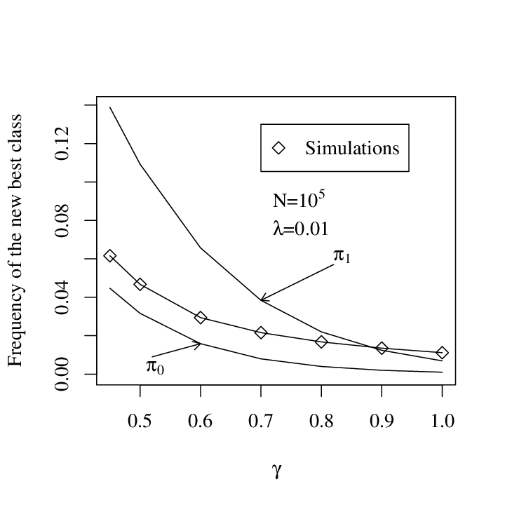
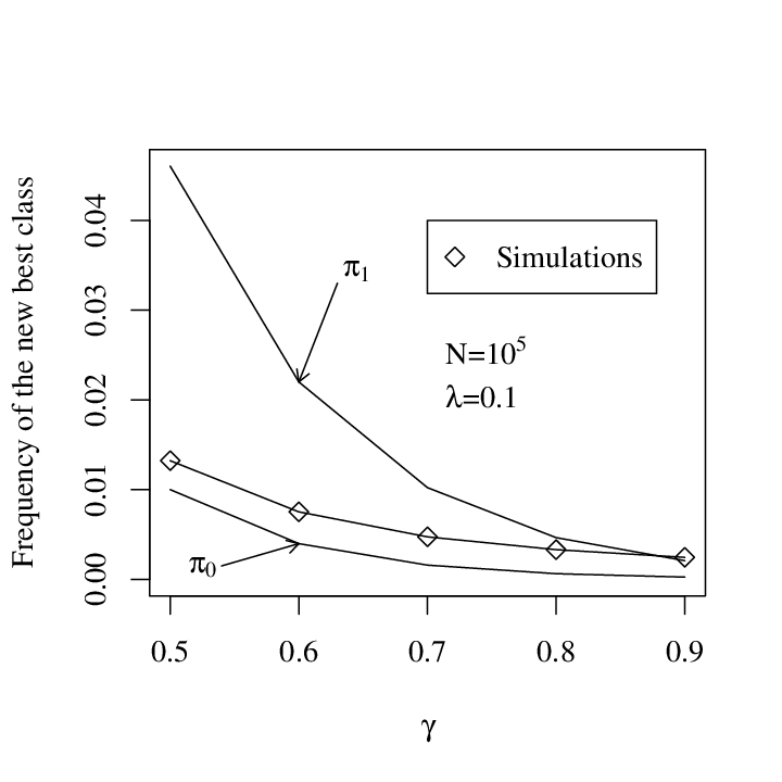
Our prediction that we observe profiles which are well approximated by a relaxed PPA applies especially well at click times. We check this numerically by observing the frequency of the (new) best class at click times; see Figure 7. For small the ratchet clicks rarely and the system has some time to relax to its new equilibrium even before the click of the ratchet. As a consequence, we see that the frequency of the (new) best class at the time of the click is already close to . However, if is large and the ratchet clicks frequently, the dynamical system has no time before the click to relax the system to the new equilibrium. Therefore, we observe that the frequency of the new best class is close to .
7 Discussion
Haigh (1978) was the first to attempt a rigorous mathematical analysis of the ideas of Muller (1964). However, in spite of the apparent simplicity of Haigh’s mathematical formulation of the model, the exact rate of Muller’s ratchet remains elusive. In this note, we have developed arguments in the spirit of Haigh (1978), Stephan et al. (1993) and Gordo & Charlesworth (2000) to give approximations for this rate.
Haigh gave the empirical formula
for the average time between clicks of the ratchet (where time is measured in generations). A quantitative understanding of the rate was first obtained by Stephan et al. (1993) using diffusion approximations and later extended by Gordo & Charlesworth (2000). Both obtain the diffusion (5.6b) as the main equation giving a valid approximation for the frequency path of the best class.
The reasoning leading to (5.6b) in these papers is twofold. Stephan et al. (1993) and Stephan & Kim (2002) argue that although fitness decreases by during one ‘cycle’ of the discrete ratchet model from §2 (in which the system advances from one Poisson equilibrium to the next), at the actual click time only a fraction of the fitness has been lost. They suggest for or as the loss of fitness at click times. In other words they predict the functional relationship discussed in §5 by linear interpolation between and ; compare with Figure 3. On the other hand, Gordo & Charlesworth (2000) use a calculation of Haigh which tells us that if the dynamical system (2.1) is started in from (2.4), then at the end of phase one (corresponding in the continuous setting, as we observed in Remark 4.3, to time ) we have . This leads to the approximation and again interpolating linearly using gives (5.6b).
Simulations show that (5.6b) provides a good approximation to the rate of the ratchet for a wide range of parameters; see e.g. Stephan and Kim (2002). The novelty in our work is that we derive (5.6b) explicitly from the dynamical system. In particular, we do not use a linear approximation, but instead derive a functional linear relationship in Proposition 4.4. In addition, we clarify the rôle of the two different phases suggested by Haigh. As simulations show, since phase one is fast, it is already complete at the time when phase two starts. Therefore, in practice, we observe states that are relaxed PPAs.
The drawback of our analysis is that we cannot give good arguments for the choice of in (5.3b) and (5.6b). However, note that the choice of is essential to obtain the prefactor of 0.58 in (5.3b). E.g., if , the choice of leads to a prefactor of 0.13 while leads to the prefactor of 0.95, neither of which fits with simulated data; see Figure 6.
We obtain two more diffusion approximations, which are valid in the cases of frequent and rare clicking, respectively. In practice, both play little rôle in the prediction of the rate of the ratchet. For fast clicking, (5.6b) shows the same power law behaviour as (5.6a) and rare clicks are never observed in simulations.
Of course from a biological perspective our mathematical model is very naive. In particular, it is unnatural to suppose that each new mutation confers the same selective disadvantage and, indeed, not all mutations will be deleterious. Moreover, if one is to argue that Muller’s ratchet explains the evolution of sex, then one has to quantify the effect of recombination. Such questions provide a rich, but challenging, mathematical playground.
Acknowledgements We have discussed Muller’s ratchet with many different people. We are especially indebted to Ellen Baake, Nick Barton, Matthias Birkner, Charles Cuthbertson, Don Dawson, Wolfgang Stephan, Jay Taylor and Feng Yu.
References
- Bürger, (1991) Bürger, R. (1991). Moments, cumulants and polygenic dynamics. J. Math. Biol., 30:199–213.
- Charlesworth, (1978) Charlesworth, B. (1978). Model for evolution of Y chromosomes and dosage compensation. Proc. Natl. Acad. Sci. USA, 75(11):5618–5622.
- Charlesworth, (1996) Charlesworth, B. (1996). The evolution of chromosomal sex determination and dosage compensation. Curr. Biol., 6:149–162.
- Charlesworth and Charlesworth, (1997) Charlesworth, B. and Charlesworth, D. (1997). Rapid fixation of deleterious alleles can be caused by Muller’s ratchet. Genet. Res., 70:63–73.
- Charlesworth and Charlesworth, (1998) Charlesworth, B. and Charlesworth, D. (1998). Some evolutionary consequences of deleterious mutations. Genetica, 102/103:2–19.
- Gessler, (1995) Gessler, D. D. (1995). The constraints of finite size in asexual populations and the rate of the ratchet. Genet. Res., 66(3):241–253.
- Gordo and Charlesworth, (2000) Gordo, I. and Charlesworth, B. (2000). The degeneration of asexual haploid populations and the speed of Muller’s ratchet. Genetics, 154(3):1379–1387.
- Haigh, (1978) Haigh, J. (1978). The accumulation of deleterious genes in a population–Muller’s Ratchet. Theor. Popul. Biol., 14(2):251–267.
- Higgs and Woodcock, (1995) Higgs, P. G. and Woodcock, G. (1995). The accumulation of mutations in asexual populations and the structure of genealogical trees in the presence of selection. J. Math. Biol., 33:677–702.
- Lambert, (2005) Lambert, A. (2005). The branching process with logistic growth. Ann. Appl. Probab, 15(2):1506–1535.
- Loewe, (2006) Loewe, L. (2006). Quantifying the genomic decay paradox due to Muller’s ratchet in human mitochondrial DNA. Genet. Res., 87:133–159.
- Maia et al., (2003) Maia, L. P., Botelho, D. F., and Fontatari, J. F. (2003). Analytical solution of the evolution dynamics on a multiplicative fitness landscape. J. Math. Biol., 47:453–456.
- Maynard Smith, (1978) Maynard Smith, J. (1978). The Evolution of Sex. Cambridge University Press.
- Rice, (1994) Rice, W. (1994). Degeneration of a non-recombining chromosome. Science, 263:230–232.
- Stephan et al., (1993) Stephan, W., Chao, L., and Smale, J. (1993). The advance of Muller’s ratchet in a haploid asexual population: approximate solutions based on diffusion theory. Genet. Res., 61(3):225–231.
- Stephan and Kim, (2002) Stephan, W. and Kim, Y. (2002). Recent applications of diffusion theory to population genetics. In Modern Developments in Theoretical Population Genetics, Oxford University Press, pages 72–93.