Two-Dimensional Fluctuating Vesicles in Linear Shear Flow
Abstract
The stochastic motion of a two-dimensional vesicle in linear shear flow is studied at finite temperature. In the limit of small deformations from a circle, Langevin-type equations of motion are derived, which are highly nonlinear due to the constraint of constant perimeter length. These equations are solved in the low temperature limit and using a mean field approach, in which the length constraint is satisfied only on average. The constraint imposes non-trivial correlations between the lowest deformation modes at low temperature. We also simulate a vesicle in a hydrodynamic solvent by using the multi-particle collision dynamics technique, both in the quasi-circular regime and for larger deformations, and compare the stationary deformation correlation functions and the time autocorrelation functions with theoretical predictions. Good agreement between theory and simulations is obtained.
pacs
87.16.DgMembranes, bilayers, and vesicles and 87.15.YaFluctuations and 67.40.HfHydrodynamics in specific geometries, flow in narrow channels1 Introduction
The dynamics of soft objects such as drops, capsules and cells in flow represents a long-standing problem in science and engineering, but has received increasing interest recently, in particular due to its relevance to biological, medicinal and microfluidic applications. This problem is challenging from a theoretical point of view, because the shape of these objects is not given a priori, but determined dynamically from a balance of interfacial forces with fluid stresses. Improved experimental methods have revealed intriguing new dynamical shape transitions due to the presence of shear flow. The phenomenology of the dynamical behavior depends distinctively on the specific soft object immersed in the flow with fluid bilayer vesicles and elastic microcapsules as the most prominent classes.
Fluid bilayer vesicles assume a stationary tank-treading shape in linear shear flow, if there is no viscosity contrast between interior and exterior fluid Kraus et al. 1996. If the interior fluid or the membrane becomes more viscous, a transition to a tumbling state can occur Biben and Misbah 2003; Beaucourt et al. 2004a; Rioual et al. 2004; Noguchi and Gompper 2004; Noguchi and Gompper 2005a; Vlahovska and Gracia 2007. Tank-treading was observed experimentally in infinite shear flow de Haas et al. 1997; Kantsler and Steinberg 2005 and for vesicles interacting with a rigid wall Lorz et al. 2000; Abkarian et al. 2002, where a dynamic lift occurs Seifert 1999a; Cantat and Misbah 1999; Sukumaran and Seifert 2001; Beaucourt et al. 2004b. The tank-treading to tumbling transition was observed for the first time convincingly in an experiment only very recently Kantsler and Steinberg 2006. In addition to the tank-treading to tumbling transition, an oscillating motion was predicted theoretically Misbah 2006 and observed experimentally Kantsler and Steinberg 2006 and in simulations Noguchi and Gompper 2007. This type of motion has alternatively been called vacillating-breathing Misbah 2006, swinging Noguchi and Gompper 2007, or trembling Kantsler and Steinberg 2006; Lebedev et al. 2007. The theoretical description has been extended recently beyond first order in the shear rate Noguchi and Gompper 2007; Lebedev et al. 2007; Danker et al. 2007.
At finite temperature, stochastic fluctuations of the membrane due to thermal motion affect the motion of the object. Due to the dissipative nature of the hydrodynamic interactions, vesicles in shear flow form a non-trivial model system for studying non-equilibrium stochastic dynamics. Since the effect of thermal noise on the transitions between the different modes of motion in general is a challenging task, in this paper we concentrate on the stochastic motion in the stationary tank-treading state. Our theoretical approach is similar to that of Ref. Seifert 1999b, where stochastic equations of motion were derived for quasi-spherical vesicles.
Most numerical methods solving the equation of motion of vesicles or capsules Kraus et al. 1996; Biben and Misbah 2003 operate in the absence of thermal forces. An exception, which naturally includes thermal noise, is multi-particle collision dynamics (MPC), also known as stochastic rotation dynamics (SRD) Malevanets and Kapral 1999; Malevanets and Kapral 2000; Kikuchi et al. 2003; Yeomans 2006. In this method, the fluid part is modeled on a particle rather than a continuum level. The microscopic equations of motion for the effective fluid are chosen to be evaluated efficiently on the one hand, and on the other hand to lead to the correct macroscopic hydrodynamics. This method has successfully been applied to flow around rigid objects Lamura et al. 2001; Lamura and Gompper 2002, polymers Kikuchi et al. 2005; Ripoll et al. 2006 and viscous vesicles Noguchi and Gompper 2004; Noguchi and Gompper 2005a; Noguchi and Gompper 2005b; Noguchi and Gompper 2007. We employ the MPC simulation method to compare our theoretical predictions of correlation functions, inclination angles, and tank-treading frequencies with simulation data of vesicles. In order to obtain good statistics, we focus here on two-dimensional (2d) vesicles with a linear boundary.
The paper is organized as follows: After formulating the problem in section 2, we develop nonlinear stochastic equations of motion for quasi-circular vesicles in section 3. These are solved approximately using a mean field approach and a low temperature expansion in section 4. We also present the 2d version of the deterministic Keller-Skalak theory Keller and Skalak 1982 in section 5, which takes into account the influence of the vesicle shape on the flow. The simulation method used is discussed in section 6. Finally we compare the calculations with simulation data in section 7 and discuss our results.
2 Problem formulation
We consider a model 2d vesicle immersed in a fluid of viscosity with a 1d membrane boundary surrounding a fluid of viscosity and at finite temperature . Due to the incompressibility of the membrane and of the enclosed fluid, the area and the length of the membrane are constants. The membrane resists deformation with a bending rigidity , which is defined rigorously below in section 2.1. The fixed area defines a length scale
| (1) |
which can be used to define a number of dimensionless quantities. In the following, we use the excess length
| (2) |
and the dimensionless viscosity contrast
| (3) |
Alternatively one can derive a length from the length constraint, and use it to define a reduced area . The reduced area is connected to the excess length by
| (4) |
In a quiescent fluid, thermal stochastic forces acting on the membrane lead to a fluctuating shape, where the probability of any specific deformation can be calculated using the Boltzmann weight corresponding to the deformation energy . If an external flow field is switched on, the system ceases to be in equilibrium, and the statistical weight of a deformation cannot be calculated a priory using Boltzmann weights. We first derive the force balance governing the motion of a vesicle in stochastic Stokes flow, before we simplify the equations of motion in the limit of small deformations from a circular shape.
2.1 Constitutive equation of the membrane
We employ conventions of differential geometry following Ref. do Carmo 1976. The shape of the vesicle is given by the shape function , where denotes the arc length. The tangent vector is of unit length. The unit normal vector is defined to point to the outside of the vesicle, and the orientation is chosen such that the pair forms a right handed system. The curvature is defined via the relation
| (5) |
The 2d analog of the bending energy of a certain membrane deformation is given by the Helfrich term Helfrich 1973
| (6) |
which corresponds also to the bending energy of a semi-flexible polymer Kratky and Porod 1949. Note that for 3d vesicles, a spontaneous curvature can appear in the bending energy for intrinsically asymmetric monolayers or asymmetric liquid environments. In 2d vesicles, we can ignore the spontaneous curvature, since it shifts the bending energy only by a topological constant, much like the Gaussian curvature contribution to the curvature energy can be ignored in 3d.
All deformations of the vesicle must preserve the length . In addition, the fluid membrane is locally incompressible. This is ensured by introducing the tension as a Lagrange parameter. The total energy thus reads
| (7) |
From the Euler-Lagrange equations we can deduce the force acting on the membrane
| (8) |
Here the prime denotes a derivative with respect to the arc length .
2.2 Stochastic Stokes flow
The elastic forces given by Eq. (8) are balanced by hydrodynamic forces mediated by the surrounding fluid. The motion of the fluid and the vesicle is only considered on time scales on which the fluid is incompressible, i.e.
| (9) |
The length and time scales in typical experiments and simulations is such that the Reynolds number is very small. We only consider fluctuations on time scales on which the inertial term in the Navier-Stokes equation can be neglected. The velocity field of the fluid is then subject to the steady stochastic Stokes equation Landau and Lifshitz 1959
| (10) |
where the thermal stress tensor is assumed to be a Gaussian random variable with zero mean and correlations
| (11) |
Here indicates the inner or outer fluid. Instead of calculating the stochastic velocity field of the flow, we only calculate the deterministic part of :
| (12) |
At the vesicle membrane we must have force balance between the deterministic and stochastic part of the hydrodynamic force and the elastic forces
| (13) |
Here, denotes the deterministic hydrodynamic stress tensor with Cartesian components
| (14) |
Far away from the vesicle the velocity field assumes the externally given values
| (15) |
which is ensured by separating an induced part from the velocity field
| (16) |
and requiring that the induced part drops to zero far away from the vesicle. Assuming no-slip boundary conditions, the vesicle is advected by the flow, which implies
| (17) |
Here the dynamics still depends implicitly on , which has to be chosen such that remains the arc length, ensuring incompressibility. Eqs. (8,12–17) determine the stochastic motion of the vesicle.
3 Quasi-circular approximation
These equations can be simplified considerably if we restrict ourselves to vesicle shapes close to the circle. We parameterize the shapes as a function of the polar angle
| (18) |
and consider small distortions . The deformation amplitude is a real periodic function of and can therefore be expanded into complex Fourier modes
| (19) |
For comparison with simulation data described below, an expansion into a real Fourier series is advantageous. We therefore also employ the expansion
| (20) |
The real Fourier coefficients are connected with the complex Fourier coefficients via ()
| (21) |
Area conservation fixes in terms of the other
| (22) |
This relation will be used throughout the paper, and from now on sums over exclude the term. The contour length of the membrane is calculated to second order in to be
| (23) |
Hence the excess length reads
| (24) |
Finally, the local curvature evaluates to
| (25) |
This leads to the bending energy (ignoring constant terms)
| (26) |
We now add the global length constraint (24) with a Lagrangian multiplier
| (27) |
to the quadratic part of the bending energy. This leads to a quadratic expression for the total energy (88)
| (28) |
with
| (29) |
The bending forces (8) are determined by the deformation amplitudes and by the instantaneous tension
| (30) |
The homogeneous tension has already been included into the energy (28).
3.1 Velocity field
In polar coordinates, the general solution of Stokes’ equation can be expanded into the fundamental modes Happel and Brenner 1983
| (31) |
In this representation the cases and are special and have to be treated separately. They correspond to constant flow and rotational flow, respectively. The deeper reason why these are special cases is the Stokes paradox Happel and Brenner 1983. It follows from the boundary conditions that the induced velocity field on the inside must be composed of “” modes, and of “” modes on the outside.
The corresponding hydrodynamic stress tensor reads in components
| (32) |
and
| (33) |
We can now express the 2d Oseen tensor in spectral components. The radial and polar components of the fluid velocity and hydrodynamic force at the reference circle are expanded into Fourier modes analogous to the expansion (19). The velocity field at the reference sphere together with the boundary conditions uniquely determines the expansion (31). From the spatial velocity field the hydrodynamic force can be calculated, leading to
| (34) |
3.2 External flow
In the absence of the vesicle the applied external flow must be regular everywhere. Therefore apart from constant flow and constant rotation only the “+” modes contribute in the expansion (31). To avoid the intricacies of the Stokes paradox, we neglect the possibility of constant flow. A general expansion of the external flow therefore reads
| (35) |
The last term in this expansion corresponds to rotational flow with the vorticity . For a finite viscosity contrast there is a jump in the traction
| (36) |
For the specific case of external linear shear flow
| (37) |
we can read off the only non-vanishing components
| (38) |
We will also use the dimensionless shear rate
| (39) |
and vorticity
| (40) |
3.3 Incompressibility condition
The flow at the vesicle membrane is subject to the incompressibility condition , which can be cast in the equivalent form . To leading order in the deformation, this condition reads
| (41) |
Separating the induced flow from the external flow, we have in Fourier components
| (42) |
Using this relation, we can eliminate and obtain
| (43) |
3.4 Equation of motion
Neglecting the thermal fluctuating forces for the moment, we can derive a deterministic equation of motion. The force balance leads to
| (44) |
with
| (45) |
and
| (46) |
From the induced velocity, we obtain the radial component of the full velocity field
| (47) |
The advection equation then reads (cf. Ref. Seifert 1999b)
| (48) |
with
| (49) |
At non-zero temperature, thermal forces must be taken into account in the force balance. The deterministic equation of motion (48) then becomes a Langevin equation
| (50) |
The form of the thermal noise can be obtained directly from the noise term in Eq. (13). It is much easier, however, to determine from the Einstein relation, which must be valid in equilibrium. We assume that the equilibrium noise is valid also for non-vanishing shear flow and choose
| (51) |
Eq. (50) is the correct stochastic equation of motion for the vesicle deformation modes . The tension is at each instance determined such that the length constraint (24) is fulfilled. Taking the time derivative of Eq. (24) and using Eq. (50), we can solve for the tension
| (52) |
When this expression is inserted back into Eq. (50), the resulting noise term becomes dependent on the instantaneous values of the . While such non-linear noise terms hold interesting physics, we first concentrate on tractable approximate solutions to the stochastic equation of motion.
4 Approximate solutions
4.1 Mean-field treatment
At finite temperature, higher-order modes are excited by stochastic thermal forces and therefore cannot be neglected. The full non-linear set of Langevin equations (50) in combination with the expression (52) for is too complex to admit a general solution. We can, however, gain further insight in the tank-treading regime using a mean-field description. We replace the fluctuating tension in Eq. (50) by a constant, which has to be determined self-consistently from the length constraint. The Langevin equations (50) then become linear and decouple. In the stationary state, only the deformations have a finite mean,
| (53) |
On average, the vesicle is elliptical. As a measure of the deformation from the circle we define the Taylor deformation parameter
| (54) |
where and denote the long and short axis of the ellipse. In the mean-field treatment we have
| (55) |
The inclination angle is obtained from Eq. (53)
| (56) |
The deviations from the mean
| (57) |
obey the homogeneous Langevin equation
| (58) |
The stationary noise correlations are best evaluated using a time Fourier transform
| (59) |
leading to
| (60) |
We can solve for and obtain the correlations
| (61) |
We have left the -dependence of implicit for clarity. The time correlation function becomes ()
| (62) |
with the stationary equal-time correlations
| (63) |
The amplitudes with different are uncorrelated at all times. Comparison with simulation data is easier using the real Fourier coefficients (20). The corresponding correlation functions read
| (64) |
and
| (65) |
The fluctuating contribute to the excess length according to Eq. (24). Although the length constraint cannot be obeyed exactly with a constant tension, we determine such that the constraint (24) is fulfilled on average. The total excess length has a systematic and a fluctuating part
| (66) |
with
| (67) |
and
| (68) |
Thus is determined implicitly by the solution of Eq. (66). For future reference, we note that the contribution of the fluctuating parts to the excess length can be determined analytically to be
| (69) |
While this expression is exact, its behavior as a function of is not obvious (for example, the “singularities” at and are only apparent). We therefore give the leading asymptotic behavior
| (70) |
4.2 Zero temperature
At large shear rates, nearly the entire excess length is stored in the systematic part . As a crossover shear rate , we can define the shear rate at which the two contributions in condition (66) become equal
| (71) |
This set of equations must be solved numerically for each . In the limit we can ignore the thermal forces. In this case, the equation of motion (50) becomes the deterministic Eq. (48), and the tension is determined by Eq. (52) with .
We can easily obtain the stationary state from , i.e.
| (72) |
The homogeneous tension is determined from the length constraint (24). In the case of constant linear shear flow, only the components are non-zero and are equal in magnitude. The length constraint thus reads , or
| (73) |
The homogeneous tension in the stationary state is thus given by
| (74) |
vanishes at a critical viscosity ratio
| (75) |
This corresponds to a tank-treading to tumbling transition, as can be seen when we allow for time-dependent : In linear shear flow, only the modes are excited. In the long time limit we can therefore assume that all other modes have decayed. In analogy with the 3d treatment Misbah 2006, we can write in polar form
| (76) |
where is the inclination angle of the vesicle with respect to the shear direction. Taking the real and imaginary part of Eq. (48) gives the familiar Jeffery’s equation Jeffery 1922
| (77) |
For , Eq. (77) admits two stationary solutions, of which only the positive is linearly stable
| (78) |
This corresponds to stationary tank-treading motion, where the tank-treading frequency at zeroth order is given by the external flow
| (79) |
For , the right hand side of Eq. (77) is always negative, and the vesicle starts to tumble. In two dimensions, no analogy to a swinging motion (cf. Refs. Misbah 2006; Kantsler and Steinberg 2006; Noguchi and Gompper 2007; Lebedev et al. 2007) exists, since the volume and length constraint already uniquely determine the shape of an ellipse.
4.3 First-order correction to the large shear-rate limit
In the mean-field approach the tension is assumed constant and all modes fluctuate independently with amplitudes given by Eq. (63). In this picture, the length constraint is not fulfilled rigorously but only on average. For strictly enforced length constraint the tension must fluctuate according to Eq. (52), which induces correlations between the deformation amplitudes. While this general effect is worth considering in its own right, here we concentrate on the much simpler large shear rate (or low temperature) limit as a perturbation of the deterministic solution.
At , the whole excess length is stored in the mode. Perturbing the modulus of the amplitude alters the excess length to first order and is prohibited by the constraint (2). Perturbing the other modes alters only to second order. At low temperature, we can therefore assume the polar decomposition (76). Taking the real and imaginary part of the equation of motion (50), we arrive at a Langevin equation for the inclination angle
| (80) |
where the noise term
| (81) |
is Gaussian and delta-correlated
| (82) |
In the stationary regime fluctuates around the mean value
| (83) |
where is given by Eq. (78). For small we can expand Eq. (80) to obtain
| (84) |
This implies the stationary correlations
| (85) |
where we have used Eq. (78). For small we read off
| (86) |
Finally, we calculate the fluctuations of the Fourier modes . The polar expansion (76) implies
| (87) |
We derive the correlation functions of the modes from Eq. (85) to be
| (88) |
5 Keller-Skalak theory
In the theory of Keller and Skalak Keller and Skalak 1982, a three-dimensional vesicle is assumed to have a fixed ellipsoidal shape
| (89) |
where the are the semi-axes of the ellipsoid, and the coordinate axes point along its principal directions. The and axes, with , are chosen to lie in the plane and are rotated through an angle with respect to the and axes. The components of the undisturbed shear flow are . The velocity field at the membrane is assumed to be
| (90) |
where is a parameter having the dimensions of a frequency. The energy supplied by the external flow has to be balanced with the energy dissipated inside the vesicle. The motion of the vesicle derived from this energy balance reads Keller and Skalak 1982
| (91) |
with
| (92) |
and
| (93) |
The factors appearing in Eqs. (91)-(93) are given by
| (94) |
and
| (95) |
For , we obtain a steady tank-treading angle
| (96) |
We calculate the inclination angle and the tank-trading frequency by adapting the Keller-Skalak theory to two dimensions. We numerically solve Eqs. (91)-(93) in the limit keeping finite, which formally corresponds to an ellipsoid with an infinite semi-axis in the direction.
6 Simulation method
A 2d vesicle model system was simulated using the multi-particle collision (MPC) dynamics Malevanets and Kapral 1999; Noguchi and Gompper 2004; Yeomans 2006. In this method the fluid is not treated on a continuum level, but rather by a stochastic dynamics of effective fluid particles.
6.1 Solvent dynamics
We consider a two-dimensional system made of identical particles of mass whose positions and velocities , , are continuous variables. The time is discretized in intervals . The evolution occurs in two consecutive steps, streaming and collision. In the streaming step, particles move ballistically,
| (97) |
For the collision step, the system is divided into the cells of a regular square lattice of mesh size . Each of these cells is the interaction area where an instantaneous multi-particle collision occurs, which changes particles velocities as Malevanets and Kapral 1999
| (98) |
where is the average velocity of the colliding particles in a cell. The velocity field is considered to be the macroscopic velocity of the fluid and it is assumed to have the coordinates of the center of the cell. denotes a stochastic rotation matrix which rotates, with equal probability, by an angle of either or . The collisions are performed simultaneously on all the particles in a cell with the same rotation , but may differ from cell to cell. The local momentum and kinetic energy are conserved under this dynamics. The kinetic energy of particles fixes the temperature , where is the Boltzmann constant, via the equipartition theorem.
It was shown in Ref. Ripoll et al. 2004 that a proper description of hydrodynamics in MPC requires large Schimdt numbers. This can be accomplished by choosing a mean-free path , which is small compared to the cell size . It is known that a value of much smaller than breaks the Galilean invariance Ihle and Kroll 2001 and that this problem can be solved by applying a random shift procedure Ihle and Kroll 2001. The viscosity of the solvent fluid is Kikuchi et al. 2003; Ihle et al. 2004
| (99) |
with particle density and number of particles per cell.
In order to enforce shear flow, we place our system of size between two horizontal walls. The upper and the lower walls slide along the direction with velocities and , respectively, with . Periodic boundary conditions are used along the direction. Along the direction, we use a modified bounce-back boundary condition which consists in requiring that particles hitting the walls change their velocities according to . Together with virtual particles in partly filled cells at walls, this describes no-slip boundary conditions very well Lamura et al. 2001; Lamura and Gompper 2002. A linear flow profile is obtained with shear rate , with the walls placed at . The relative velocities in the collision cells are rescaled after each time step in order to keep the temperature constant in the (driven) system.
6.2 Membrane model
The vesicle membrane is modeled by connecting beads of mass successively with bonds into a closed ring. Neighboring beads along the closed chain are connected to each other with the harmonic potential
| (100) |
where is a spring constant, is the position vector of the -th bead, and is the average bond length. The bending energy (26) is modeled on the discrete level by a bending potential
| (101) |
where is the angle between successive bonds. The fluid modeled with the MPC method is compressible. To enforce the area constraint in the presence of thermal and hydrodynamic forces, we add a constraint potential
| (102) |
6.3 Coupling of membrane and solvent dynamics
The membrane-solvent interaction must prevent solvent particles from crossing the membrane and enforce no-slip boundary conditions on the membrane. Therefore we place hard disks centered on the membrane beads. The disk radius is set in order to ensure overlapping of disks and a complete coverage of the membrane. The exchange of momentum between the solvent particles and the membrane occurs in the following way. After updating beads positions and velocities via molecular dynamics (MD), we freely stream all the solvent particles. We then execute bounce-back scattering between solvent and membrane disks only when a solvent particle and a disk satisfy the conditions and . This means that if the two collision partners and overlap and move towards each other, then their velocities are updated according to
| (103) |
To avoid that a solvent particle moves too far inside a disk, we require that . The collision step (98) is performed only on those solvent particles which did not scatter. If the collision step were executed also on the scattered solvent particles, they might continue to collide with the same disk in the next time step. The fluids in the interior and exterior of the vesicle are taken to be the same, in particular to have the same viscosity.
A chain of disks of finite radius has an inner length available to the solvent particles which is smaller than the outer length. Since the solvent has the same density inside and outside, the outer fluid exerts a compression force on the membrane until the inner density increases so that an expansion force compensates the compression one. It is straightforward to show Noguchi and Gompper 2005a that the density increase is where is the effective membrane thickness. This requires that is large enough compared to the disk radius to reduce such compression effects. The number of solvent particles placed inside the vesicle fixes an average area. However, since the MPC fluid is compressible, shear and bending rigidity effects may change the area . For this reason the constraint potential (102) is introduced to keep the area constant.
6.4 Parameters
In experiments with vesicles in shear flow, inertial effects are negligible since the Reynolds number is very small. We express our results using the reduced area , defined in Eq. (4), and the reduced shear rate , see Eq. (39), as relevant dimensionless quantities.
We set , , and . This implies a viscosity . We use , , , and such that for all the cases we considered with . Finally, we set , , , , , , , . The area is chosen in such a way that . With the choices for and the area and the length of the vesicle are kept constant with a deviation of less than of the target values for all simulated systems. A snapshot of a simulated vesicle and the resulting velocity field for the reduced area and reduced shear rate is shown in Fig. 1.
7 Results and discussion
7.1 Stationary deformations
In Fig. 2 we show the stationary deformation correlations , as a function of the mode number for and . We also show a fit of these correlations for with the theoretical prediction (65). From the fit we can extract the tension . In this particular example we obtain , whereas theory predicts from Eqs. (66)–(68).
7.2 Tension vs shear rate
Fig. 3 shows the extracted dimensionless tensions for different dimensionless shear rates and for two different excess lengths and . The agreement with the theoretical prediction from a numerical solution of Eqs. (66)–(68) is satisfactory. The fact that this function is nearly a straight line implies that the large-shear-rate approximation (14) is valid down to small shear rates. We find a crossover shear rate , below which there are deviations from a linear behavior. Theoretically, Eq. (71) gives an order-of-magnitude estimate of for and for .
7.3 Autocorrelation function
In Fig. 4, the time autocorrelation function is shown as a function of dimensionless time . The data follows the expected exponential decay (64) very well. From the amplitude we can extract a tension , while from the time constant we deduce . Theory predicts . Given the rather noisy data, this agreement seems reasonable. For moderate shear rates the autocorrelation function has decayed before the oscillations implied by Eq. (64) become noticeable. Even for the large shear rate used in Fig. 4, the oscillations are barely visible. For the same reason the build up of cross correlation is hidden in the numerical noise.
7.4 Inclination angle
We compare the averaged inclination angle for different reduced areas with Eq. (78) in Fig. 5, valid in the quasi-circular limit. The agreement with simulation data is satisfactory, given the large error bars. The 2d Keller-Skalak theory, which is also shown in the plot, gives slightly better agreement.
In Fig. 6, we show the fluctuations of the inclination angle as a function of the shear rate. The theoretical scaling is given by Eq. (86), and is in excellent agreement for (), (), and (). The scaling of the fluctuations of for differs significantly for (). In the deterministic case, a vesicle with such a low reduced area would tumble within the quasi-circular theory. This implies that the quasi-circular approximation works well for (corresponding to ) in two dimensions.
7.5 Tank-treading frequency
8 Summary
We have studied the fluctuations and deformation of a 2d vesicle in shear flow at finite temperature. In the limit of small deformations from a circle, we have derived analytical Langevin-type equations of motion, which are nonlinear due to the length constraint. A mean-field treatment allows approximate predictions for the stationary correlation functions and time autocorrelation functions of the deformation amplitudes, which agree quantitatively with simulation data. Deviations of the stationary correlations from the mean-field predictions in the lowest mode are explained quantitatively in a low temperature expansion of the original constrained Langevin equations. The mean inclination angle and the tank-treading frequency are better described by a deterministic 2d Keller-Skalak theory. Fluctuations of the inclination angle are also determined quantitatively. Theory and simulations agree well for low excess lengths, but differ for larger excess lengths.
The good quantitative agreement of mesoscale simulations of vesicles in flow with detailed theoretical calculations demonstrates the predictive power of these simulation methods for more complex flow geometries.
Acknowledgements.
RF, US and GG would like to acknowledge financial support through the DFG priority program SPP 1146 “Micro- and Nanofluidics”. AL and GG acknowledge fruitful discussions with H. Noguchi, M. Ripoll, G. Vliegenthart, and R. Winkler. AL thanks Gerhard Gompper and co-workers for hospitality at the Forschungszentrum Jülich and acknowledges support from CNR through the Short-Term Mobility Program.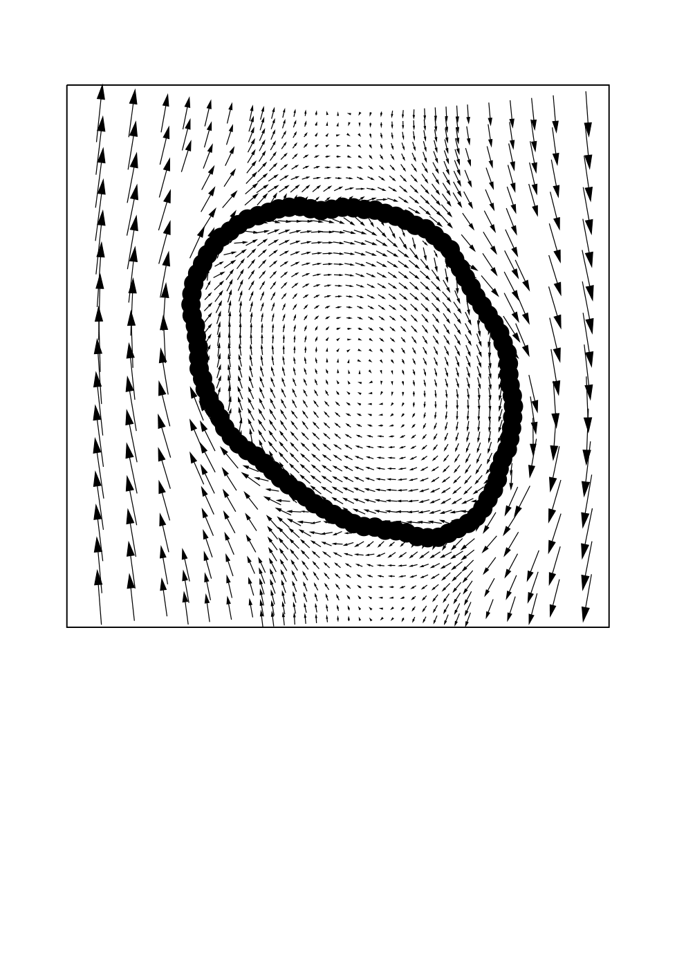


References
- Kraus et al. (1996) M. Kraus, W. Wintz, U. Seifert, and R. Lipowsky, Phys. Rev. Lett. 77, 3685 (1996).
- Biben and Misbah (2003) T. Biben and C. Misbah, Phys. Rev. E 67, 031908 (2003).
- Beaucourt et al. (2004a) J. Beaucourt, F. Rioual, T. Seon, T. Biben, and C. Misbah, Phys. Rev. E 69, 011906 (2004a).
- Rioual et al. (2004) F. Rioual, T. Biben, and C. Misbah, Phys. Rev. E 69, 061914 (2004).
- Noguchi and Gompper (2004) H. Noguchi and G. Gompper, Phys. Rev. Lett. 93, 258102 (2004).
- Noguchi and Gompper (2005a) H. Noguchi and G. Gompper, Phys. Rev. E 72, 011901 (2005a).
- Vlahovska and Gracia (2007) P. M. Vlahovska and R. S. Gracia, Phys. Rev. E 75, 016313 (2007).
- de Haas et al. (1997) K. de Haas, C. Blom, D. van den Ende, M. H. G. Duits, and J. Mellema, Phys. Rev. E 56, 7132 (1997).
- Kantsler and Steinberg (2005) V. Kantsler and V. Steinberg, Phys. Rev. Lett. 95, 258101 (2005).
- Lorz et al. (2000) B. Lorz, R. Simson, J. Nardi, and E. Sackmann, Europhys. Lett. 51, 468 (2000).
- Abkarian et al. (2002) M. Abkarian, C. Lartigue, and A. Viallat, Phys. Rev. Lett. 88, 068103 (2002).
- Seifert (1999a) U. Seifert, Phys. Rev. Lett. 83, 876 (1999a).
- Cantat and Misbah (1999) I. Cantat and C. Misbah, Phys. Rev. Lett. 83, 880 (1999).
- Sukumaran and Seifert (2001) S. Sukumaran and U. Seifert, Phy. Rev. E 64, 11916 (2001).
- Beaucourt et al. (2004b) J. Beaucourt, T. Biben, and C. Misbah, Europhys. Lett. 67, 676 (2004b).
- Kantsler and Steinberg (2006) V. Kantsler and V. Steinberg, Phys. Rev. Lett. 96, 36001 (2006).
- Misbah (2006) C. Misbah, Phys. Rev. Lett. 96, 28104 (2006).
- Noguchi and Gompper (2007) H. Noguchi and G. Gompper, Phys. Rev. Lett. 98, 128103 (2007).
- Lebedev et al. (2007) V. V. Lebedev, K. S. Turitsyn, and S. S. Vergeles, arXiv:cond-mat/0702650v1 (2007).
- Danker et al. (2007) G. Danker, T. Biben, T. Podgorski, C. Verdier, and C. Misbah, arXiv:cond-mat/0703698v2 (2007).
- Seifert (1999b) U. Seifert, Eur. Phys. J. B 8, 405 (1999b).
- Malevanets and Kapral (1999) A. Malevanets and R. Kapral, J. Chem. Phys. 110, 8605 (1999).
- Malevanets and Kapral (2000) A. Malevanets and R. Kapral, J. Chem. Phys. 112, 7260 (2000).
- Kikuchi et al. (2003) N. Kikuchi, C. M. Pooley, J. F. Ryder, and J. M. Yeomans, J. Chem. Phys. 119, 6388 (2003).
- Yeomans (2006) J. M. Yeomans, Physica A 369, 159 (2006).
- Lamura et al. (2001) A. Lamura, G. Gompper, T. Ihle, and D. M. Kroll, Europhys. Lett. 56, 319 (2001).
- Lamura and Gompper (2002) A. Lamura and G. Gompper, Eur. Phys. J. E 9, 477 (2002).
- Kikuchi et al. (2005) N. Kikuchi, J. F. Ryder, C. M. Pooley, and J. M. Yeomans, Phys. Rev. E 71, 061804 (2005).
- Ripoll et al. (2006) M. Ripoll, R. G. Winkler, and G. Gompper, Phys. Rev. Lett. 96, 188302 (2006).
- Noguchi and Gompper (2005b) H. Noguchi and G. Gompper, Proc. Natl. Acad. Sci. USA 102, 14159 (2005b).
- Keller and Skalak (1982) S. R. Keller and R. Skalak, J. Fluid. Mech. 120, 27 (1982).
- do Carmo (1976) M. do Carmo, Differential Geometry of Curves and Surfaces (Englewood Cliffs, NJ: Prentice Hall, 1976).
- Helfrich (1973) W. Helfrich, Z. Naturf. C 28, 693 (1973).
- Kratky and Porod (1949) O. Kratky and G. Porod, Rec. Trav. Chim. 68, 1106 (1949).
- Landau and Lifshitz (1959) L. D. Landau and E. M. Lifshitz, Fluid mechanics, vol. 6 (London, Pergamon Press, 1959).
- Happel and Brenner (1983) J. Happel and H. Brenner, Low Reynolds number hydrodynamics (The Hague, Martinus Nijhoff Publishers, 1983).
- Jeffery (1922) G. B. Jeffery, P. Roy. Soc. A 102, 161 (1922).
- Ripoll et al. (2004) M. Ripoll, K. Mussawisade, R. G. Winkler, and G. Gompper, Europhys. Lett. 68, 106 (2004).
- Ihle and Kroll (2001) T. Ihle and D. M. Kroll, Phys. Rev. E 63, 020201(R) (2001).
- Ihle et al. (2004) T. Ihle, E. Tüzel, and D. M. Kroll, Phys. Rev. E 70, 035701(R) (2004).