Entropy production by Q-ball decay for diluting long-lived charged particlesPreprint: DESY 07-146
Abstract
The cosmic abundance of a long-lived charged particle such as a stau is tightly constrained by the catalyzed big bang nucleosynthesis. One of the ways to evade the constraints is to dilute those particles by a huge entropy production. We evaluate the dilution factor in a case that non-relativistic matter dominates the energy density of the universe and decays with large entropy production. We find that large Q balls can do the job, which is naturally produced in the gauge-mediated supersymmetry breaking scenario.
I Introduction
Gauge-mediated supersymmetry (SUSY) breaking (GMSB) GMSB is appealing since the problems associated with the dangerous flavor-changing processes and CP violations are elegantly solved. In this scenario, the gravitino mass is lighter than the weak scale and therefore the gravitino is most probably the lightest supersymmetric particle (LSP). If the -parity is conserved, the gravitino LSP is absolutely stable and can be a good candidate for dark matter (DM) Moroi:1993mb; Bolz:1998ek; Bolz:2000fu; Ellis:2003dn; Steffen:2006hw; Takahashi:2007tz. In addition, such a scenario with a light gravitino may lead to spectacular collider signatures especially if the next-to-lightest superparticle (NLSP) is a electrically charged particle such as a stau. The stau NLSP has a quite long life time, since the decay rate is suppressed by the Planck scale GeV). Such longevity may enable us to measure the Planck scale at collider experiments and therefore to test supergravity BHRY, if the gravitino mass is GeV.
However, the existence of such long-lived charged particles can jeopardize the success of the big bang nucleosynthesis (BBN). Since the stau decays during or after BBN, the energetic decay products may alter the primordial abundance of the light elements Kawasaki:2004yh; Jedamzik:2004er. Furthermore, it was recently found that the negatively charged (long-lived) particle can form bound states with nuclei (e.g., 4He) , which catalyze the nuclear reactions and substantially change the abundance of the light elements such as 6Li Pospelov:2006sc. The detailed discussion based on the catalyzed BBN (CBBN) limits the life time of the stau as sec, assuming the thermal relic abundance for the stau. Taking the upper bound at face value, we are led to smaller and/or heavier , which are challenging from the experimental point of view or on the basis of naturalness.
To alleviate the BBN constraints, several solutions (e.g., -parity violation Buchmuller:2007ui) has been proposed. Among them, it is simplest to assume that there is late-time entropy production to dilute the stau abundance. According to Ref. HHKKY, the necessary dilution factor is for GeV, where denotes the stau mass. However, successful late-time entropy production is not so easily achieved as one might think of. The reason is as follows com-by-TY. To be concrete, we assume that the gravitino is LSP while the stau is NLSP, and that a scalar field with even -parity produces large entropy. Then the scalar mass must be lighter than , since the supersymmetric partners of the standard-model (SM) particles, if kinematically allowed, are generically produced from the decay of Endo:2006zj; Endo:2006ix. In addition, since is lighter than the stau mass, must be more strongly coupled to the SM particles than the gravitational interactions †† † This ameliorates a possible gravitino production from the scalar field Endo:2006ix., in order to decay before BBN. On the other hand, the fermionic partner of must be heavier than , because we have assumed that the stau is NLSP. Therefore the mass spectrum must satisfy , where is the mass of the fermionic partner of . To realize such spectrum, however, one needs a partial cancellation between the SUSY mass and the soft SUSY breaking mass. Thus, it is difficult, if not impossible, to naturally induce a late-time entropy production in the set-up with the gravitino LSP and the stau NLSP.
In this article, we show that the successful entropy production can be achieved by the decay of the Q ball in the minimal supersymmetric SM (MSSM). In our scenario, a large charge naturally makes the effective mass smaller than and it also explains the longevity of the Q ball. Since the fermionic partners are nothing but the SM particles, there is no constraint on the fermion mass. In addition, a right amount of the baryon asymmetry can be generated by the Affleck-Dine (AD) mechanism FD; DRT.
In the next section, we provide a brief review on the Q balls in GMSB. We estimate the dilution factor in both cases when the Q ball dominates the universe after and before the freeze-out of the stau in Sec. III. In Sec. IV, we show that the Q-ball decay can dilute the stau by the desired amount. In Sec. V we give our conclusion and discussions.
II Q ball in GMSB
A Q ball is a non-topological soliton of a complex scalar field given by the minimum energy configuration with a fixed charge Coleman:1985ki. One of the conditions for the Q balls to be formed is that the scalar potential with a symmetry is shallower than the quadratic potential at large field value. The Q balls are known to be formed associated with the scalar dynamics of the MSSM fields, especially in connection with the AD mechanism FD; DRT. In addition, since the Q balls generically have a very long life time, they can play important roles in cosmology.
In MSSM, there are many flat directions composed of some combination of squarks, sleptons and Higgs bosons. Along the flat directions, both -term and -term potentials vanish in the exact SUSY limit at renormalizable level DRT; Gherghetta:1995dv. They are lifted by the soft SUSY breaking effects, non-renormalizable operators, and finite temperature effects. In the AD mechanism, one of the flat directions (denoted by ) is assumed to have a large field value during inflation ‡‡ ‡ Actually, multiple flat directions can have large expectation values simultaneously, but we do not consider this possibility for simplicity. . After inflation, starts to oscillate when the Hubble parameter becomes comparable to the mass of . At the same time, acquires the baryon (and/or lepton) asymmetry, due to non-renormalizable baryon-(lepton-)number violating operators that are effective only at large field values. The scalar potential of has an approximate symmetry corresponding to the baryon and lepton symmetries that are conserved at low energy effective theory, i.e., MSSM. As we will see below, since the scalar potential is shallower than the quadratic potential above the messenger scale in GMSB, experiences spatial instabilities and deforms into Q balls, where the charge corresponds to the baryon and/or lepton numbers.
As mentioned above, the scalar potential is lifted by the SUSY breaking effects, non-renormalizable operators, and finite temperature effects. In GMSB, the scalar potential above the messenger scale is given by
| (1) |
where is the gravitino mass, GeV is the reduced Planck scale, and we omit the baryon-(lepton-)number violating operators here. The first term comes from the GMSB effect above the messenger scale deGouvea. and are related to the and components of a gauge-singlet chiral multiplet in the messenger sector as
| (2) |
respectively, where collectively stands for the SM gauge couplings, and denotes the Yukawa coupling constant between and the messenger fields. In general, could be in the range GeV GeV for GeV. The second term of Eq. (1) comes from the gravity-mediated SUSY breaking, and the coefficient is of the order unity. Here the one-loop correction is included, and is negative with for most of the flat directions. Since the gravitino mass is relatively small in the gauge mediation, this term is effective for a large field value of . The third term in the potential is due to a non-renormalizable interaction in the superpotential of the form with , where is a coupling constant. The fourth term is a two-loop thermal correction to the potential thermal. The coefficient can be both positive and negative depending on which flat direction we choose KKT1, and the absolute value is roughly given by , where we define . The last term is a Hubble-induced mass term, which stems from the quartic coupling in the Kähler potential between the flat direction and the inflaton DRT. This term is absent after the reheating of the inflaton. Because of this term, the potential has a minimum at a large field amplitude during inflation, and the field is trapped there and it serves as the initial condition for the later dynamics §§ § The same effect may be realized by large enough Hubble-induced A terms Aterm.. To be concrete, we assume throughout this paper that the minimum is given by the balance between the Hubble-induced mass term and the non-renormalizable operator:
| (3) |
where . The flat direction traces the minimum until it starts to oscillate.
After inflation, the flat direction starts rotating, experiences spatial instability, and deforms into Q balls Qball1; Qball2; KK1; KK2; KK3. The properties of the Q ball are well known. The charge is determined by the amplitude of the field at the onset of the oscillations, . If the potential at is dominated by the first or fourth term in Eq.(1), the charge of the Q ball, which is called the gauge-mediation type, is determined as KK3
| (4) |
where is defined as
| (5) |
The subscript “” denotes that the variable should be evaluated at the onset of the oscillation of . The numerical coefficient is given by KK1; KK3
| (6) |
where denotes the ratio of the baryon number density to the number density of . The size and mass of the Q ball, and the effective mass of the field inside the Q ball (i.e., the mass per unit charge) are written respectively as Qball1; KK3
| (7) |
On the other hand, if the potential at is dominated by the second term in Eq.(1), the gravity-mediation type of Q ball is formed, whose charge is given by Newtype; KK3
| (8) |
where
| (9) |
The size and mass of the Q ball, and the effective mass of the field inside the Q ball (i.e., the mass per unit charge) are written respectively as Qball2; Newtype; KK3
| (10) |
The Q ball can decay if the mass per unit charge is larger than the decay products that carry the same charge. For example, if is the baryon number, the lightest particle with baryonic charge is a nucleon whose mass is GeV. Therefore, such Q balls with GeV can decay into the nucleons (perhaps together with other lighter particles such as -mesons). Since the decay can proceed only from the surface of the Q ball, the decay rate is bounded from above. For the MSSM Q ball, the rate is saturated and given by Qdecay
| (11) |
Therefore, the decay temperature of the Q ball is calculated as
where counts the relativistic degrees of freedom at the Q-ball decay, and we define in the second equality.
III Estimate of Dilution factor
Let us now estimate how much the abundance of the stau is diluted in a situation that the Q ball releases entropy after it dominates the energy density of the universe. We define the dilution factor as
| (15) |
where the left-hand side represents the ratio of the stau number density to the entropy density in the presence of the entropy production due to the Q-ball decay, while the abundance of the stau on the right-hand side is estimated without the entropy production. Note that, although we consider the Q-ball decay, our arguments in this section can be applied to any scenario that non-relativisitc matter dominates the universe and decays with large entropy production.
The stau abundance can be diluted if the Q-ball decay takes place after the freeze-out of the stau. The dilution factor depends on the thermal history. We assume that the universe is radiation-dominated before the Q balls start to dominate the energy density of the universe. Let us define , , and as the temperatures when the Q-ball energy density becomes equal to the radiation density, the stau freezes out, and the Q ball decays, respectively. (We will use such notation that the subscripts , , and denote that the variables should be estimated at and , respectively.) In Fig. 1 we sketch the evolution of the energy densities of the radiation, the Q ball, and the radiation produced by the Q-ball decay.
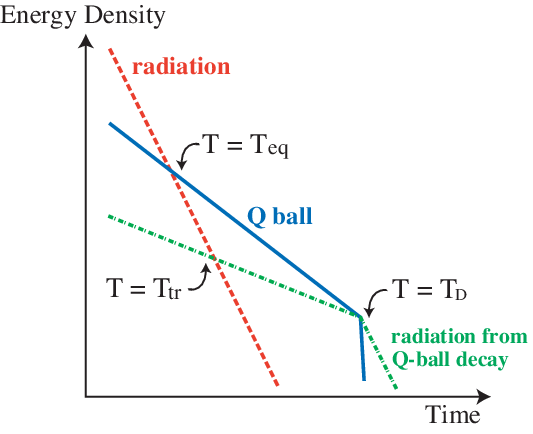
We now consider the following cases: (i) and (ii) . In the case (i), the situation is very simple, since the Q balls change the evolution of the universe after the freeze-out of the stau. We thus obtain
| (16) |
The dilution factor is calculated as
| (17) | |||||
where is the energy density of the Q balls.
In the latter case (ii), the stau decouples from thermal equilibrium when the Q ball is dominating the universe. Therefore one needs to know the dependence of the stau number density on the Hubble parameter at the freeze-out. Since the freeze-out takes place when the annihilation rate becomes comparable to the expansion rate, we obtain
| (18) |
where is the thermally averaged cross section for the stau annihilation processes. The freeze-out temperature becomes larger than that in the usual radiation-dominated universe, since the energy density at the freeze-out is higher in the presence of the Q balls. However the change in is not significant, because the stau decouples when it is non-relativistic, so the freeze-out temperature is rather insensitive to the change in the cosmic expansion rate. Thus, we simply assume in the following ¶¶ ¶ To include the change in , let us define , where denotes the freeze-out temperature for the modified cosmic expansion. It is estimated as for the case B, and for the case C (See Eq.(22) and Fig. 1). The freeze-out temperature does not change in the case A. As long as we stick to , the minimum values of are given by , and our approximation seems to be valid. To take account of this change in , one has to multiply in Eq.(22) by in the cases B and C with replaced with . Then, one can see that becomes larger by a factor of at most. Note that including the effect always increases the dilution factor. . Such an approximation is not essential to our arguments. Then we can estimate as
| (19) | |||||
where we use at the freeze-out, and denotes the Hubble parameter at the freeze-out in the absence of the Q-balls.
The relation betwen the Hubble parameter, , and the freeze-out temperature, , depends on whether the newly created radiation from the Q-ball decay dominates over the radiation that was present from the beginning, at the freeze-out of the stau. Let denote the transition temperature at which both radiation components become comparable to each other. (See Fig. 1.) In the case of , we have
| (20) |
where we use and . On the other hand, in the case of , we have . Substituting this into Eq. (19), we obtain
| (21) |
In summary, we find that the dilution factor is given as follows depending on when the freeze-out takes place:
| (22) |
Note that the decay temperature should lie in the range of MeV LowTRH and it must satisfy , in order to dilute the stau by the entropy production.
In the next section, we will determine the Q-ball-radiation equality temperature by considering the formation and the dynamics of Q balls, in order to evaluate the dilution factor .
IV Entropy production by the Q-ball decay
The Q-ball formation and the subsequent thermal history depend on the scalar potential at the onset of the oscillations. Since the large charge Q ball is necessary for a long lifetime, the field amplitude at the onset of the oscillation should be very large. In that case, the zero-temperature potential would be dominated by the gravity-mediation term (the second term in Eq.(1)). As we will see below, the thermal corrections are negligible for the parameters we adopt in the following analysis.
The flat direction starts to oscillate when . Here we simply assume that it takes place when the inflaton oscillation dominates the energy density of the universe. Then the ratio of the energy densities of the Q ball and the inflaton at the reheating is given by
| (23) |
After reheating the ratio evolves as , so the Q-ball-radiation equality temperature is obtained as
| (24) |
Meanwhile the decay temperature is calculated from Eq.(II) as
| (25) |
where and are used. Since the freeeze-out temperature is GeV for GeV, the dilution factor is estimated as in the case A:
| (26) |
In this case we have . Notice that shown in (25) can marginally satisfy the BBN constraints LowTRH. For slightly larger or smaller , one can have a large enough that safely satisfies the BBN bound, keeping the dilution factor large enough. Since the initial amplitude of the flat direction is determined as in Eq.(3), it will be realized for the direction ( or ) with , or the direction () with . The coefficient of the thermal logarithmic corrections will be negative for these directions. If the thermal correction to the potential dominates over the gravity-mediation term, it will spoil the above scenario because the field will be trapped by the negative thermal logarithmic potential, and so, it cannot be released for a long time. In order to avoid such a situation, we must impose a condition that the thermal logarithmic correction is negligible at the onset of the oscillations: ∥∥ ∥ The thermal logarithmic term may not appear in such situation that the dilute plasma before reheating is suppressed because of e.g., the small mass of the inflaton and/or the existence of appropriate multiple flat directions. . Using , it is rewritten as
| (27) |
which is satisfied in the above analysis.
Finally, we comment on the last moment of the Q-ball decay. As the charge becomes small, the gravity-mediation type Q ball gradually deforms into the gauge-mediation type one. Therefore, at a certain point, the mass per unit charge of the Q ball may exceed the stau mass, , which implies that the stau can be produced. In order to suppress the stau abundance as , we must impose GeV. This is because and the branching ratio is estimated as where . Such a small value of is realized in a model where the Yukawa coupling is suppressed as in the case of the composite field.
V Conclusion
We have shown that the Q-ball decay can produce large enough entropy to dilute the cosmic abundance of a long-lived charged particle such as a stau. Since the Q balls are composed of the MSSM particles, our scenario is minimal in some sense. Successful late-time entropy production is not so easily achieved as one might think of: the particle that produces entropy should have a smaller mass than the stau and a long lifetime, and no unwanted particle production should occur. In our scenario, a large charge naturally makes the effective mass smaller than the stau mass, and the decay products are just the SM particles. It also explains the longevity of the Q ball. The large Q ball can be naturally produced in the dynamics of the flat direction.
In addition, we have derived analytically the dilution factor for the cases that the stau freezes out both before and after the Q ball starts to dominate the universe.
Lastly let us briefly discuss the baryon asymmetry and the dark matter. Due to the late-time entropy production, the baryon asymmetry and the gravitino dark matter are also diluted. One way out is to over-produce both by the amount of the dilution beforehand. Another is to create them after the entropy production. As for the gravitino dark matter, the thermal production does not suffice since the reheating temperature cannot be too high due to the constraint (27). Therefore, one has to rely on the non-thermal production Takahashi:2007tz; Kawasaki:2006gs. On the other hand, one can obtain a right magnitude of the baryon asymmetry from the Q-ball decay itself, making use of the Affleck-Dine baryogensis. If the flat direction has the baryon number, it must start the oscillations with suppressed angular motion (i.e., ). On the other hand, for the leptonic direction, the lepton charges evaporated from the Q ball before the electroweak phase transition are partially converted into the baryon asymmetry through the sphaleron processes. In this case, is necessary to have a right abundance of the baryon asymmetry.
Acknowledgments
SK is grateful to M. Kawasaki for useful discussion. FT thanks M. Endo for discussion. The work of SK is supported by the Grant-in-Aid for Scientific Research from the Ministry of Education, Science, Sports, and Culture of Japan, No. 17740156.
References
- (1) M. Dine, A. E. Nelson and Y. Shirman, Phys. Rev. D 51 (1995) 1362; M. Dine, A. E. Nelson, Y. Nir and Y. Shirman, Phys. Rev. D 53 (1996) 2658; For a review, see, for example, G. F. Giudice and R. Rattazzi, Phys. Rep. 322 (1999) 419, and references therein.
- (2) T. Moroi, H. Murayama and M. Yamaguchi, Phys. Lett. B 303, 289 (1993).
- (3) M. Bolz, W. Buchmüller and M. Plümacher, Phys. Lett. B 443, 209 (1998).
- (4) M. Bolz, A. Brandenburg and W. Buchmüller, Nucl. Phys. B 606, 518 (2001).
- (5) J. R. Ellis, K. A. Olive, Y. Santoso and V. C. Spanos, Phys. Lett. B 588, 7 (2004); L. Roszkowski, R. Ruiz de Austri and K. Y. Choi, JHEP 0508, 080 (2005); D. G. Cerdeño, K. Y. Choi, K. Jedamzik, L. Roszkowski and R. Ruiz de Austri, JCAP 0606, 005 (2006).
- (6) F. D. Steffen, JCAP 0609, 001 (2006).
- (7) F. Takahashi, arXiv:0705.0579 [hep-ph].
- (8) W. Buchmüller, K. Hamaguchi, M. Ratz and T. Yanagida, Phys. Lett. B 588, 90 (2004).
- (9) M. Kawasaki, K. Kohri and T. Moroi, Phys. Lett. B 625, 7 (2005); M. Kawasaki, K. Kohri and T. Moroi, Phys. Rev. D 71, 083502 (2005).
- (10) K. Jedamzik, Phys. Rev. D 70, 063524 (2004).
- (11) M. Pospelov, Phys. Rev. Lett. 98, 231301 (2007); K. Kohri and F. Takayama, arXiv:hep-ph/0605243; M. Kaplinghat and A. Rajaraman, Phys. Rev. D 74, 103004 (2006); R. H. Cyburt, J. Ellis, B. D. Fields, K. A. Olive and V. C. Spanos, JCAP 0611, 014 (2006); K. Hamaguchi, T. Hatsuda, M. Kamimura, Y. Kino and T. T. Yanagida, Phys. Lett. B 650, 268 (2007); C. Bird, K. Koopmans and M. Pospelov, arXiv:hep-ph/0703096; M. Kawasaki, K. Kohri and T. Moroi, Phys. Lett. B 649, 436 (2007); T. Jittoh, K. Kohri, M. Koike, J. Sato, T. Shimomura and M. Yamanaka, arXiv:0704.2914 [hep-ph].
- (12) W. Buchmüller, L. Covi, K. Hamaguchi, A. Ibarra and T. Yanagida, JHEP 0703, 037 (2007).
- (13) K. Hamaguchi, T. Hatsuda, M. Kamimura, Y. Kino and T. T. Yanagida, in Refs. Pospelov:2006sc
- (14) This argument is partly based on the comment by T. Yanagida at “Miniworkshop on Superweakly Interacting Dark Matter” which was held at DESY in Dec. 2006.
- (15) M. Endo, K. Hamaguchi and F. Takahashi, Phys. Rev. Lett. 96, 211301 (2006); S. Nakamura and M. Yamaguchi, Phys. Lett. B 638, 389 (2006).
- (16) M. Endo and F. Takahashi, Phys. Rev. D 74, 063502 (2006).
- (17) I. Affleck and M. Dine, Nucl. Phys. B 249, 361 (1985).
- (18) M. Dine, L. Randall and S. Thomas, Nucl. Phys. B 458, 291 (1996).
- (19) S. R. Coleman, Nucl. Phys. B 262, 263 (1985) [Erratum-ibid. B 269, 744 (1986)].
- (20) T. Gherghetta, C. F. Kolda and S. P. Martin, Nucl. Phys. B 468, 37 (1996).
- (21) A. de Gouvêa, T. Moroi and H. Murayama, Phys. Rev. D 56, 1281 (1997).
- (22) A. Anisimov and M. Dine, Nucl. Phys. B 619, 729 (2001); M. Fujii, K. Hamaguchi and T. Yanagida, Phys. Rev. D 63, 123513 (2001).
- (23) S. Kasuya, M. Kawasaki and F. Takahashi, Phys. Lett. B 578, 259 (2004).
- (24) S. Kasuya and M. Kawasaki, Phys. Rev. D 74, 063507 (2006). S. Kasuya, J. Phys. A 40, 6999 (2007) [arXiv:hep-ph/0610428].
- (25) A. Kusenko and M. E. Shaposhnikov, Phys. Lett. B 418, 46 (1998).
- (26) K. Enqvist and J. McDonald, Phys. Lett. B 425, 309 (1998); K. Enqvist and J. McDonald, Nucl. Phys. B 538, 321 (1999).
- (27) S. Kasuya and M. Kawasaki, Phys. Rev. D 61, 041301(R) (2000).
- (28) S. Kasuya and M. Kawasaki, Phys. Rev. D 62, 023512 (2000).
- (29) S. Kasuya and M. Kawasaki, Phys. Rev. D 64, 123515 (2001).
- (30) S. Kasuya and M. Kawasaki, Phys. Rev. Lett. 85, 2677 (2000).
- (31) A. G. Cohen, S. R. Coleman, H. Georgi and A. Manohar, Nucl. Phys. B 272, 301 (1986).
- (32) M. Kawasaki, K. Kohri and N. Sugiyama, Phys. Rev. Lett. 82, 4168 (1999); M. Kawasaki, K. Kohri and N. Sugiyama, Phys. Rev. D 62, 023506 (2000); S. Hannestad, Phys. Rev. D 70, 043506 (2004); K. Ichikawa, M. Kawasaki and F. Takahashi, Phys. Rev. D 72, 043522 (2005).
- (33) M. Kawasaki, F. Takahashi and T. T. Yanagida, Phys. Lett. B 638, 8 (2006); M. Kawasaki, F. Takahashi and T. T. Yanagida, Phys. Rev. D 74, 043519 (2006); M. Endo, M. Kawasaki, F. Takahashi and T. T. Yanagida, Phys. Lett. B 642, 518 (2006); M. Endo, F. Takahashi and T. T. Yanagida, arXiv:hep-ph/0701042; M. Endo, F. Takahashi and T. T. Yanagida, arXiv:0706.0986 [hep-ph].