Charged lepton distributions as a probe of
contact
interactions
at a linear collider with polarized beams
Kumar Rao and Saurabh D. Rindani
Theoretical Physics Division, Physical Research Laboratory
Navrangpura, Ahmedabad 380009, India
Abstract
We examine very general four-point interactions arising from new physics and contributing to the Higgs production process . We write all possible forms for these interactions consistent with Lorentz invariance. We allow the possibility of CP violation. Contributions to the process from anomalous and interactions studied earlier arise as a special case of our four-point amplitude. We consider the decay of into a charged lepton pair and obtain expressions for angular distributions of charged leptons arising from the interference of the four-point contribution with the standard-model contribution. We take into account possible longitudinal or transverse beam polarization likely to be available at a linear collider. We examine several correlations which can be used to study the various form factors present in the contact interactions. We also obtain the sensitivity of these correlations in constraining the new-physics interactions at a linear collider operating at a centre-of-mass energy of 500 GeV with longitudinal or transverse polarization.
1 Introduction
Despite the dramatic success of the standard model (SM), an essential component of SM responsible for generating masses in the theory, viz., the Higgs mechanism, as yet remains untested. The SM Higgs boson, signalling symmetry breaking in SM by means of one scalar doublet of , is yet to be discovered. A scalar boson with the properties of the SM Higgs boson is likely to be discovered at the Large Hadron Collider (LHC). However, there are a number of scenarios beyond the standard model for spontaneous symmetry breaking, and ascertaining the mass and other properties of the scalar boson or bosons is an important task. This task would prove extremely difficult for LHC. However, scenarios beyond SM, with more than just one Higgs doublet, as in the case of minimal supersymmetric standard model (MSSM), would be more amenable to discovery at a linear collider operating at a centre-of-mass (cm) energy of 500 GeV. We are at a stage when the International Linear Collider (ILC), seems poised to become a reality [1].
Scenarios going beyond the SM mechanism of symmetry breaking, and incorporating new mechanisms of CP violation, have also become a necessity in order to understand baryogenesis which resulted in the present-day baryon-antibaryon asymmetry in the universe. In a theory with an extended Higgs sector and new mechanisms of CP violation, the physical Higgs bosons are not necessarily eigenstates of CP. In such a case, the production of a physical Higgs can proceed through more than one channel, and the interference between two channels can give rise to a CP-violating signal in the production.
Here we consider in a general model-independent way the production of a Higgs mass eigenstate through the process . This is an important mechanism for the production of the Higgs, the other important mechanisms being and proceeding via vector-boson fusion. is generally assumed to get a contribution from a diagram with an -channel exchange of . At the lowest order, the vertex in this diagram would be simply a point-like coupling (Fig. 1). Interactions beyond SM can modify this point-like vertex by means of a momentum-dependent form factor, as well as by adding more complicated momentum-dependent forms of anomalous interactions considered in [2, 3, 4, 5, 6, 7, 8, 9]. The corresponding diagram is shown in Fig. 2, where the anomalous vertex is denoted by a blob. There could also be a diagram with a photon propagator and an anomalous vertex, which does not occur in SM at tree level, and which we do not show separately. We consider here a beyond-SM contribution represented by a four-point coupling shown in Fig. 3. This is general enough to include the effects of the diagram in Fig. 2. Such a discussion would be relevant in studying effects of box diagrams with new particles, or diagrams with -channel exchange of new particles, in addition to -channel diagrams.
We write down the most general form for the four-point coupling consistent with Lorentz invariance. We do not assume CP conservation. We then obtain angular distributions for a lepton pair from the decay of the calculated from the square of amplitude for the diagram in Fig. 1 with a point-like coupling, together with the cross term between and the amplitude for the diagram in Fig. 3. We neglect the square of , assuming that this new physics contribution is small compared to the dominant contribution . We include the possibility that the beams have polarization, either longitudinal or transverse. While we have restricted the actual calculation to SM couplings in calculating , it should be borne in mind that in models with more than one Higgs doublet this amplitude would differ by an overall factor depending on the mixing among the Higgs doublets. Thus our results are trivially applicable to such extensions of SM, by an appropriate rescaling of the coupling.
In our analysis, we do not assume that the is produced on shell. Moreover, since we obtain fully analytical expressions for the distribution of the final-state leptons arising from the virtual using the full propagator, we automatically take into account coherently spin correlations of the .


We are thus addressing the question of how well the form factors for the four-point coupling can be determined from the observation of decay-lepton angular distributions in the presence of unpolarized beams or beams with either longitudinal or transverse polarizations. A similar question taking into account a new-physics contribution which merely modifies the form of the vertex has been addressed before in several works [2, 3, 4, 5, 6, 7, 8, 9, 10]. Those works which do take into account four-point couplings, do not do so in all generality, but stop at the lowest-dimension operators [5]. See, however, [11], where the contribution of dimension-six operators to the processes and are considered. The approach we adopt here has been used for the process in [12, 13] and for the process in [14].
The four-point couplings, in the limit of vanishing electron mass, can be neatly divided into two types – chirality-conserving (CC) ones and chirality-violating (CV) ones. The CC couplings involve an odd number of Dirac matrices sandwiched between the electron and positron spinors, whereas the CV ones come from an even number of Dirac matrices. Since in practice, CV couplings are usually proportional to the fermionic mass (in this case the electron mass), we concentrate on the CC ones (see, however, [15]).
In an earlier work [16], we considered angular distributions of an on-shell in the process in the same context of contact interactions. In that paper we concentrated on CP-odd asymmetries constructed with the polar and azimuthal angles, for both chirality-conserving and chirality-violating cases. The present work is an extension to the more realistic case of a virtual decaying into a pair of charged leptons, which are observed. We also do not restrict ourselves to CP-odd asymmetries, but aim at the determination of all form factors in the chirality-conserving case using expectation values of CP-even and CP-odd observables. Charged-lepton angular distributions have been discussed earlier in [17] for the SM Higgs, in the context of distinguishing between a scalar and pseudoscalar Higgs in [2, 7, 8, 10, 18], and in the context of CP-violating Higgs in [3, 4, 5, 6, 7, 9, 10]. However, these papers, with the exception of [5], do not discuss contact interactions which is the topic of our work.
Polarized beams are likely to be available at a linear collider, and several studies have shown the importance of linear polarization in reducing backgrounds and improving the sensitivity to new effects [19]. The question of whether transverse beam polarization, which could be obtained with the use of spin rotators, would be useful in probing new physics, has been addressed in recent times in the context of the ILC [12, 15, 19, 20, 21, 22, 23, 24]. In earlier work, it has been observed that polarization does not give any new information about the anomalous couplings when they are assumed real [7]. However, in case of four-point contact interactions, we find that there are terms in the differential cross section which are absent unless both electron and positron beams are transversely polarized. Thus, transverse polarization, if available at ILC, would be most useful in isolating such terms. This is particularly significant because these terms are CP violating. Moreover, some of them are even under naive CPT, and thus would survive even when no imaginary part is present in the amplitude.
In the next section we write down the possible model-independent four-point couplings. In Section 3, we obtain the angular distributions arising from the CC couplings in the presence of beam polarization. Section 4 deals with correlations which can be used for separating various form factors and Section 5 describes the numerical results. Section 6 contains our conclusions and a discussion.
2 Form factors for the process
The most general four-point vertex for the process
| (1) |
consistent with Lorentz invariance can be written as
| (2) |
where the chirality-conserving part containing an odd number of Dirac matrices is
| (3) |
and the chirality violating part containing an even number of Dirac matrices is
| (4) | |||||
In the above expressions, , , and are form factors, and are Lorentz-scalar functions of the Mandelstam variables and for the process eq. (1). For simplicity, we will only consider the case here when the form factors are constants. is a parameter with dimensions of mass, put in to render the form factors dimensionless.
The expressions for the four-point vertices may be thought to arise from effective Lagrangians
| (5) | |||||
and
| (6) | |||||
where represents the Higgs field. The the coupling constants , , and in the Lagrangians have been promoted to form factors in momentum space when writing the vertex functions .
It may be appropriate to contrast our approach with the usual effective Lagrangian approach. In the latter approach, it is assumed that SM is an effective theory which is valid up to a cut-off scale . The new physics occurring above the scale of the cut-off may be parametrized by higher-dimensional operators, appearing with powers of in the denominator. These when added to the SM Lagrangian give an effective low-energy Lagrangian where, depending on the scale of the momenta involved, one includes a range of higher-dimensional operators up to a certain maximum dimension. Our effective theory is not a low-energy limit, so that the form factors we use are functions of momentum not restricted to low powers. Thus, the we introduce is not a cut-off scale, but an arbitrary parameter, introduced just to make the form factors dimensionless.
We thus find that there are 6 independent form factors in the chirality conserving case, and 6 in the chirality violating case. An alternative form for the above would be using Levi-Civita tensors whenever a occurs. The independent form factors then are then some linear combinations of the form factors given above. However, the total number of independent form factors remains the same.
Note that we have not imposed CP conservation in the above. The CP properties of the various terms appearing in the four-point vertices may be deduced from the CP properties of the corresponding terms in the effective Lagrangian. Thus, one can check that the terms corresponding to the couplings , , , and in the effective Lagrangian are CP violating. As a consequence, the terms corresponding to , , , and are CP violating, whereas the remaining are CP conserving. This conclusion assumes that the form factors are constants, since the couplings in the effective Lagrangian are constants. The conclusion can also be carried over when the form factors are arbitrary functions of and even functions of , where is the angle between and (or constants). This is because in momentum space, is even under CP, whereas is odd under C and even under P, and thus odd under CP.
3 Differential cross sections
We now obtain the differential cross section for the process (1) for a virtual followed by its decay into , viz.,
| (7) |
from the SM amplitude alone and from the interference between the SM amplitude and the amplitude arising from the four-point couplings of (3). We do not consider the CV case here. We ignore terms bilinear in the four-point couplings, assuming that the new-physics contribution is small. We treat the two cases of longitudinal and transverse polarizations for the electron and positron beams separately. We neglect the mass of the charged leptons . Also, we assume that the charged lepton is different from the electron. Thus, our considerations are mostly for , and they would be applicable for to the extent that the mass can be neglected.
The expression for the amplitude for (1), arising from the SM diagram of Fig. 1 with a point-like vertex, is
| (8) |
where the vector and axial-vector couplings of the to electrons are given by
| (9) |
and is the weak mixing angle.
Note that though we have used SM couplings for the leading contribution, it is trivial to modify these by overall factors for cases of other models (like two-Higgs-doublet models). Our expressions are not, however, applicable for the case when the Higgs is a pure pseudoscalar in models conserving CP, since in that case, the SM-like lowest-order couplings are absent.
We have obtained full analytical expressions for the differential cross sections to linear order in the contact interactions. The Dirac trace calculations have been checked using the analytical manipulation program FORM [25]. Since these expressions are obtained in a model-independent context, they can prove useful for future work comparing different models.
Note that though in eq. (3) we wrote the vertex for the production of a real , when we introduce the decay of the , we consider full virtuality of the , and also take into account spin correlations of the .
We choose the axis to be the direction of the momentum, and the plane to coincide with the production plane in the case when the initial beams are unpolarized or longitudinally polarized. The positive axis is chosen, in the case of transverse polarization, to be along the direction of the polarization.
3.1 Distributions for longitudinally polarized beams
The cross section for the process for longitudinal beam polarization is given by
| (10) | |||||
Here, respectively and () represent contributions of the pure SM amplitude and interference between the SM amplitude and the amplitudes coming from the couplings , (). The expressions for and are as follows. We use the notation , as already specified, and .
| (11) | |||||
| (12) | |||||
| (13) | |||||
| (14) | |||||
In the above, we have used
| (15) |
the longitudinal polarizations and of the electron and positron, respectively, and the effective polarization
| (16) |
3.2 Distributions for transversely polarized beams
For the transverse case, we take the polarization to be along the axis and that of the to be antiparallel to that of the . We define a four-vector and write the spin four-vector of the and as and respectively. As before, the cross section consists of four pieces coming from the square of the SM amplitude, proportional to , and the interference of the SM amplitude with the three contributions from , (), respectively proportional to . The expression for the cross section with transverse polarization for the beam and for the beam is
| (17) | |||||
The expressions for the various are:
| (18) | |||||
| (19) | |||||
| (20) | |||||
and
| (21) | |||||
4 Observables
| Symbol | Observable | CP | T |
|---|---|---|---|
After having obtained analytical expressions for the differential cross section, we choose observables whose expectation values can be used to constrain the form factors. We have chosen observables which have well defined CP properties. Thus, the expectation values of observables which are even under CP get contributions from , , and , with our assumption that the form factors have only dependence, and no dependence on (or that they are even functions of ). On the other hand, expectation values of observables which are odd under CP get contribution only from and . Moreover, it is important to note the behaviour of the observables under naïve time reversal T. The CPT theorem implies that observables which are CP even and T even would get contributions from only real parts of the form factors, as also those which are CP odd and T odd [26]. On the other hand, observables which are CP even and T odd, or CP odd and T even, are CPT odd. They therefore require the presence of an absorptive part in the amplitude, and hence are proportional to the imaginary parts of form factors [26].
The observables we choose are listed in Table 1, together with their CP and T properties.
We have evaluated the expectation values of the observables () for unpolarized as well as polarized beams, choosing the polarization to be 0.8 and polarization to be . The relevant phase-space integrals have been done numerically. In calculating the expectation values, we use the expressions for the differential cross sections given above to leading order in the new-physics contact interactions in the formula
| (22) |
Since the expectation values we concentrate are vanishing in SM, for consistency, we need use only the SM cross section in the denominator in eq. (22). We assume a cut-off of in the forward and backward directions on the azimuthal angles of both leptons. Such a cut-off is an experimental requirement, so as to avoid the beam pipe. However, we also explore the possibility that a suitable choice of can optimize the sensitivity. We treat both cases of longitudinal as well as transverse polarization. We take one form factor to be nonzero at a time. The expectation value of each observable for a given nonzero form factor is compared with the standard deviation of the observable in SM. This allows us to determine a limit that nonobservance of the expectation value can place on the corresponding form factor. Thus, the 90% CL (confidence level) limit on a form factor is determined by the expression
| (23) |
where is the SM cross section, the expectation value of the observable for unit value of the form factor, and is the integrated luminosity.
5 Numerical results
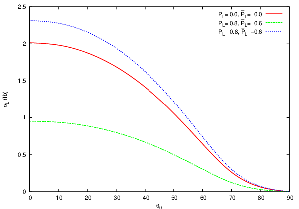
We now present out numerical results for the correlations and the limits that can be obtained from the form factors. We assume a c.m. energy of 500 GeV for the linear collider, and polarizations and respectively for the electron and positron beams. We have chosen the value of the arbitrary mass scale to be 100 GeV. We vary the cut-off .
First of all, we present the SM cross sections in the cases of unpolarized beams or longitudinal polarized beams in Fig. 4 as a function of the cut-off angle . In case of transverse beam polarization, the cross section when integrated over the azimuthal angle reduces to the unpolarized cross section [27], and hence is not shown separately.
Next, we present expectation values of some of the observables as functions of the cut-off for the purpose of illustration. The limits obtainable on the form factors, however, are presented for all observables in tables.


Fig. 5 shows the correlation for with unpolarized and longitudinally polarized beams, when Im , and the rest of the form factors are zero. Fig. 6 is the corresponding figure for Im , and the remaining form factors zero.
Similarly, Figs. 7, 8 give the correlations for for the two cases when single form factors Re and Re are respectively nonzero.


Figs. 11–16 show the expectation values of different observables for the case of transverse polarization, again, choosing one form factor nonzero at a time. The particulars of the nonzero form factors used are given in the respective figure captions.
The correlations are by and large weakly dependent on the cut-off. They vary by 10 to 20% over the whole range of .
We do not show the plot of expectation values of because they turn out to be independent of transverse polarization. Hence the expectation values can be read off from Figs. 7 and 8. This does not, however, mean that it is not useful to use transverse polarization in this case. The expectation value of the square of , which has a bearing on the sensitivity according to eq. (23), turns out to be dependent on the polarization. Thus, as will be seen below, the limit that can be obtained on Re from a measurement of can improve with transverse polarization.
Similarly, the expectation values of are very weakly dependent on transverse polarization. In Fig. 15, all the three curves corresponding to the three polarization choices lie almost on top of one another. So only the curve corresponding to is shown.
| Form | Limits for beam polarizations | ||||
| Symbol | Observable | Factor | |||
| Im | |||||
| Im | |||||
| Re | |||||
| Re | |||||
| Im | |||||
| Im | |||||
| Re | |||||
| Re | |||||
| Im | |||||
| Im | |||||
| Form | Limits for beam polarizations | ||||
| Symbol | Observable | Factor | |||
| Im | |||||
| Im | |||||
| Re | |||||
| Re | |||||
| Im | |||||
| Im | |||||
| Re | |||||
| Re | |||||
| Re | |||||
| Re | |||||
| Im | |||||
| Im | |||||
| Re | |||||
| Re | |||||
| Im | |||||
| Im | |||||
| Im | |||||
| Im | |||||
The 90% CL limits that may be obtained at the ILC running at GeV with an integrated luminosity of 500 fb-1 have been calculated for various cases using eq. (23). The results are presented in Table 2 for longitudinal polarization and in Table 3 for transverse polarization.
Table 2 shows that the best limits on all form factors using unpolarized or longitudinally polarized beams are of the order of about . Moreover, the best limits for any form factor are obtained for a suitable choice of observable when the electron and positron polarizations are opposite in sign.
Transverse polarization allows more observables to be constructed because of an additional azimuthal angle becomes available. Thus, Table 3 has more entries than Table 2. The entries which are blank in Table 3 for limits in the unpolarized case are meant to imply that the corresponding correlation is zero. These correlations which are zero in the unpolarized and longitudinal polarization cases are nonzero with transversely polarized beams. They thus give an independent measurement of certain form factors. Again, the orders of magnitude of the best limits are still around 10-4, with some cases when it is possible to go down to about .
We now make some detailed observations on our results.
gives zero expectation value in the absence of polarization if only Im and Im are nonzero. This also means that this correlation is zero for SM. This continues to be true for longitudinal polarization because, as can been seen explicitly from the expression for the cross section, the cross section does not depend on Im and Im . Hence it can be used to determine Im and Im with unpolarized beams.
With transverse polarization, the cross section does depend on imaginary parts of , and . However, the correlation vanishes when only Im and Im are nonzero.
, on the other hand, has nonzero expectation value for Re and Re , and hence for SM. It is thus more difficult to use this correlation to study new physics, though not impossible. We do not consider this correlation here.
, , and have zero expectation values with unpolarized beams. However, good sensitivity is obtained with transversely polarized beams. Of these, and have zero expectation values even with transverse polarization, when the combination of couplings corresponds to a CP-violating vertex. Thus observation of nonzero expectation value for would signal unambiguously the presence of four-point couplings we consider here.
The correlation , which is proportional to , shows strong dependence on the cut-off angle , changing sign around 25∘. Consequently, the sensitivity is low for . We have therefore chosen to evaluate the limits at for this case.
We have also varied the Higgs mass up to 350 GeV and calculated all the above correlations. However, the dependence on Higgs mass is rather weak. Thus our results hold reasonably well even for larger Higgs masses.
6 Conclusions and discussion
We have parametrized the amplitude for the process by means of form factors, using only Lorentz invariance, treating separately the chirality-conserving and chirality-violating cases. We then calculated the differential cross section for the process in terms of these form factors for polarized beams for the chirality-conserving case. The motivation was to determine the extent to which longitudinal and transverse polarizations can help in an independent determination of the various form factors.
In our earlier work [16], where we considered only angular distributions, we found that in the presence of transverse polarization, there is a CP-odd and T-odd contribution to the angular distribution. The coupling combinations this term depends on cannot be determined using longitudinally polarized beams. However, by looking at the distributions of charged leptons arising from the decay of the , we can construct CP- and T-odd correlations even in the absence of transverse polarization.
There do exist transverse-polarization dependent correlations which do not arise when only type of couplings are considered, as for example and . These correlations, if observed, would be a unique signal of CP-violating four-point interaction.
It should be emphasized that our results and conclusions are dependent on the assumption that the form factors are independent of and . In particular, the CP property of a given term in the distribution would change if the corresponding form factor is an odd function of . The reason is that is odd under CP.
We have discussed limits on the couplings that would be expected from a definite configuration of the linear collider. As for the CP-conserving couplings, limits may be obtained even from the existing LEP data, which has excluded SM Higgs up to mass of about 114 GeV. It should be borne in mind that the limits on these depend on the choice of , the arbitrary parameter of dimension of mass that we introduced.
We have looked at expectation values of observables taking only one form factor nonvanishing at a time. It must be emphasized that it feasible to extract information on form factors even when they are allowed to be nonzero independently of one another by one of two methods: Either one determines experimentally more than one correlation and solves the linear simultaneous equations for the form factors or one combines experimental information obtained with unpolarized and polarized beams to solve for the form factors. For details of this straightforward procedure, see [28, 29].
As compared to the earlier study [16] in which only the polar and azimuthal angles were considered as measurable, the use of angular variables of both leptons already presents certain new observables which give new information with even unpolarized beams, though longitudinal polarization can improve the sensitivity. The use of transverse polarization in such a situation does not present as many advantages as it did when only variables were used in asymmetries. However, if use is made of observables which involve the momentum of only one lepton at a time, transverse polarizations would again prove advantageous.
We can compare the sensitivities obtained on including decay with the sensitivities obtained using angular distributions of the itself, which were studied in [16]. There, we had used GeV, whereas here we use GeV. Keeping in mind this difference, we find that it is possible to reach similar limits using suitable correlations even in the present case. Note that in [16] what was used was asymmetries, rather than the expectation values used here.
We have also studied how our results are affected by more realistic cuts, viz., cuts on the energy of the leptons and on their transverse momentum. Since we already assume a cut on the lepton polar angles, it is not necessary to study the effect of the cut on transverse momentum separately from a cut on the energy. We find that for cuts on the energies of both leptons of 20 (30) GeV all relevant quantities (cross section, correlation and the limits on the form factors change by about 5% (10%). Thus our conclusions would remain valid fairly accurately even with experimental cuts.
We assumed that the Higgs can be detected with full efficiency. In practice, of course, the detection of the Higgs would require putting cuts on the Higgs decay products, leading to an efficiency factor less than 1. This would make our limits worse. On the other hand, some of our correlations which involve only the sum of the momenta of the leptons can also be extended to the case of hadronic decays of the . In that case, the event sample would be larger, improving the limits.
One should keep in mind the possibility that electroweak radiative corrections, which can be particularly large for transverse polarization [30], can lead to quantitative changes in the above results.
Nevertheless, we would like to emphasize that our work contains full analytical expressions for charged-lepton distributions, and can prove a useful input to a more exhaustive work taking into account, on the one hand, a variety of specific models, and on the other hand more precise experimental constraints and other practical considerations.
Though we have used SM couplings for the leading contribution of Fig. 1, as mentioned earlier, the analysis needs only trivial modification when applied to a model like MSSM or a multi-Higgs-doublet model, and will be useful in such extensions of SM. It is likely that such models will give rise to four-point contributions through box diagrams or loop diagrams with a -channel exchange of particles. However, to our knowledge, such calculations are not available for CP-violating models. The interesting effects we have discussed would make it useful to carry out such calculations.
Acknowledgment: This work was partly supported by the IFCPAR project no. 3004-2.
References
- [1] A. Djouadi, J. Lykken, K. Monig, Y. Okada, M. J. Oreglia, S. Yamashita et al., arXiv:0709.1893 [hep-ph].
- [2] Q. H. Cao, F. Larios, G. Tavares-Velasco and C. P. Yuan, Phys. Rev. D 74, 056001 (2006) [arXiv:hep-ph/0605197].
- [3] S. S. Biswal, R. M. Godbole, R. K. Singh and D. Choudhury, Phys. Rev. D 73, 035001 (2006) [arXiv:hep-ph/0509070].
- [4] T. Han and J. Jiang, Phys. Rev. D 63, 096007 (2001) [arXiv:hep-ph/0011271].
- [5] V. Barger, T. Han, P. Langacker, B. McElrath and P. Zerwas, Phys. Rev. D 67, 115001 (2003). [arXiv:hep-ph/0301097]; W. Kilian, M. Kramer and P. M. Zerwas, arXiv:hep-ph/9605437; Phys. Lett. B 381, 243 (1996) [arXiv:hep-ph/9603409].
- [6] G. J. Gounaris, F. M. Renard and N. D. Vlachos, Nucl. Phys. B 459, 51 (1996) [arXiv:hep-ph/9509316].
- [7] K. Hagiwara and M. L. Stong, Z. Phys. C 62, 99 (1994) [arXiv:hep-ph/9309248].
- [8] V. D. Barger, K. m. Cheung, A. Djouadi, B. A. Kniehl and P. M. Zerwas, Phys. Rev. D 49, 79 (1994) [arXiv:hep-ph/9306270].
- [9] K. Hagiwara, S. Ishihara, J. Kamoshita and B. A. Kniehl, Eur. Phys. J. C 14, 457 (2000) [arXiv:hep-ph/0002043].
- [10] A. Skjold and P. Osland, Nucl. Phys. B 453, 3 (1995) [arXiv:hep-ph/9502283].
- [11] J. Kile and M. J. Ramsey-Musolf, arXiv:0705.0554 [hep-ph].
- [12] B. Ananthanarayan and S. D. Rindani, Phys. Lett. B 606, 107 (2005) [arXiv:hep-ph/0410084]; JHEP 0510, 077 (2005) [arXiv:hep-ph/0507037].
- [13] K. J. Abraham and B. Lampe, Phys. Lett. B 446, 163 (1999). [arXiv:hep-ph/9810205].
- [14] K. J. Abraham and B. Lampe, Phys. Lett. B 326, 175 (1994).
- [15] S. D. Rindani, Phys. Lett. B 602, 97 (2004) [arXiv:hep-ph/0408083].
- [16] K. Rao and S. D. Rindani, Phys. Lett. B 642, 85 (2006) [arXiv:hep-ph/0605298].
- [17] C. M. J. Chen, J. W. J. Chen and W. Y. P. Hwang, Phys. Rev. D 50, 4485 (1994).
- [18] G. Mahlon and S. J. Parke, Phys. Rev. D 74, 073001 (2006) [arXiv:hep-ph/0606052].
- [19] G. Moortgat-Pick et al., arXiv:hep-ph/0507011.
- [20] T. G. Rizzo, JHEP 0302, 008 (2003) [arXiv:hep-ph/0211374]; J. Fleischer, K. Kolodziej and F. Jegerlehner, Phys. Rev. D 49, 2174 (1994); M. Diehl, O. Nachtmann and F. Nagel, Eur. Phys. J. C 32, 17 (2003) [arXiv:hep-ph/0306247]; S. Y. Choi, J. Kalinowski, G. Moortgat-Pick and P. M. Zerwas, Eur. Phys. J. C 22, 563 (2001) [Addendum-ibid. C 23, 769 (2002)] [arXiv:hep-ph/0108117].
- [21] B. Ananthanarayan and S. D. Rindani, Phys. Rev. D 70, 036005 (2004) [arXiv:hep-ph/0309260];
- [22] B. Ananthanarayan, S. D. Rindani, R. K. Singh and A. Bartl, Phys. Lett. B 593, 95 (2004) [Erratum-ibid. B 608, 274 (2005)] [arXiv:hep-ph/0404106]; J. Kalinowski, arXiv:hep-ph/0410137; P. Osland and N. Paver, arXiv:hep-ph/0507185.
- [23] A. Bartl, K. Hohenwarter-Sodek, T. Kernreiter and H. Rud, Eur. Phys. J. C 36, 515 (2004) [arXiv:hep-ph/0403265]; A. Bartl, H. Fraas, S. Hesselbach, K. Hohenwarter-Sodek, T. Kernreiter and G. Moortgat-Pick, JHEP 0601, 170 (2006) [arXiv:hep-ph/0510029]; S. Y. Choi, M. Drees and J. Song, arXiv:hep-ph/0602131; A. Bartl, K. Hohenwarter-Sodek, T. Kernreiter and O. Kittel, arXiv:0706.3822 [hep-ph]; A. Bartl, H. Fraas, K. Hohenwarter-Sodek, T. Kernreiter, G. Moortgat-Pick and A. Wagner, Phys. Lett. B 644, 165 (2007) [arXiv:hep-ph/0610431].
- [24] S. D. Rindani, arXiv:hep-ph/0409014.
- [25] J. A. M. Vermaseren, arXiv:math-ph/0010025.
- [26] See, for example, S.D. Rindani, Pramana 49, 81 (1997); Pramana 45, S263 (1995) [arXiv:hep-ph/9411398]; G. C. Branco, L. Lavoura and J. P. Silva, “CP violation,” Oxford, UK: Clarendon (1999) 511 p
- [27] K.-i. Hikasa, Phys. Rev. D 33, 3203 (1986).
- [28] P. Poulose and S. D. Rindani, Phys. Lett. B 383, 212 (1996) [arXiv:hep-ph/9606356]; Phys. Rev. D 54, 4326 (1996) [Erratum-ibid. D 61, 119901 (2000)] [arXiv:hep-ph/9509299]; Phys. Lett. B 349, 379 (1995) [arXiv:hep-ph/9410357]; F. Cuypers and S. D. Rindani, Phys. Lett. B 343, 333 (1995) [arXiv:hep-ph/9409243].
- [29] S. D. Rindani, Pramana 61, 33 (2003) [arXiv:hep-ph/0304046].
- [30] P. Ciafaloni, D. Comelli and A. Vergine, JHEP 0407 (2004) 039 [arXiv:hep-ph/0311260].