Detection of acceleration radiation in a Bose-Einstein condensate

August 11, 2026

One of the surprising fundamental consequences of relativistic quantum field theory is the dependence of the concept of particle number on the observer’s state of motion. While inertial observers see the vacuum as empty, non-inertial observers generally perceive this vacuum as populated with particles. Unruh [1] showed that a uniformly accelerated particle detector perceive the field in vacuum as a thermal state with temperature $k_{B}T_{U}=\hbar a/2\pi c$, where $a$ is the proper acceleration. The Unruh effect is related to other particle creation effects in curved space-time, such as Hawking radiation, and the Gibbons-Hawking thermalization in a cosmological expansion [2].

Numerous experimental ideas for detecting the effect have been suggested. They include, accelerated electrons in circular high energy accelerators[3], circular motion of electrons in a Paul trap[4], intense laser induced electron acceleration[5] and passage of atoms through a cavity[6]. Other setups simulate the Gibbon-Hawking cosmological expansion thermalization effect in an expanding Bose-Einstein condensate (BEC)[7], and in an expanding linear ion trap[9]. (See also [10]).

In this letter we propose to simulate and detect the Unruh effect using accelerated atom dots (AD) [11] or using optical lattices in a BEC. Since the relevant velocity is the speed of sound, $c_{s}\approx 1[mm/sec]$, $T_{U}\approx 10[nK\,sec^{2}/m]\times a[m/sec^{2}]$ and the currently feasible acceleration of optical lattices may reach $a\approx 5\times 10^{5}[m/sec^{2}]$, the Unruh temperature can be significantly higher than the relevant energy scales, the AD minimal energy gap ($\approx 100Hz\approx nK$), and the BEC temperature.

Let us begin by recalling some features of the Unruh effect. A detector is modeled as a localized system with internal levels $|g\rangle$ and $|e\rangle=\sigma^{+}|g\rangle$ and energy gap $\omega_{d}$, which moves along a trajectory $x_{D}(\tau)$ and $t(\tau)$, where $\tau$ is the detector’s proper time. In the simplest case, a free scalar field $\phi$, initially in its vacuum state, couples with the detector through

By evaluating the transition amplitudes between the levels, it is then found that for inertial trajectories the detector remains unexcited, while for uniformly accelerated trajectories the detector becomes thermalized. This can be seen by evaluating to the lowest order in $g$ the transition amplitudes. Inserting $x_{D}(\tau)={c^{2}\over a}\cosh{a\tau\over c}$, and $t(\tau)={c\over a}\sinh{a\tau\over c}$, and the expression for a free field $\phi(x,t)$ in Eq. (1), one finds that a field mode $\omega$ has a time dependent coupling of the form: $g_{e}(\tau,\omega)=\exp({i{\omega c\over a}e^{-{a\tau\over c}}})$. This readily yields transition probabilities which satisfy $P_{\rm excitation}/P_{de-excitation}=e^{-E/k_{B}T_{U}}$, where $T_{U}$ is the Unruh temperature.

It is important to note that: i. The appearance of the effective coupling $g_{e}(\tau,\omega)$ is sufficient in order to thermalize the detector. A similar coupling is also a landmark of the Hawking and cosmological thermalization effects. ii. In the Unruh effect property i. is a direct consequence of the detector’s accelerated motion. This can be easily seen [13] by noticing that the field mode $\omega$ is Doppler shifted in the detector’s rest frame to $\omega^{\prime}(\tau)=\omega_{0}{1-v/c\over\sqrt{1-(v/c)^{2}}}=\omega_{0}e^{-a\tau/c}$. Therefore, the relevant collected phase factor becomes $\exp(i\int\omega(\tau)d\tau))=g_{e}(\omega,\tau)$. iii. The Unruh effect is manifestly relativistic. Hence the interaction (1) is defined in the detector’s rest frame, and the trajectory, $x_{DR}(t)=c\sqrt{t^{2}+{c^{2}/a^{2}}}$ coincides with non-relativistic acceleration only for sufficiently short times.

The above points quantify, with increasing refinement, important aspects of the Unruh effect, which one wishes to simulate in a specific model. For example, i. can be obtained by modifying the vacuum normal mode frequencies $\omega$ to $\omega(t)=\omega e^{-{at\over c}}$, and realized in an ion traps by changing the trap frequency [9], or by an an expanding BEC [7]. In what follows we suggest a model that incorporates properties i. and ii., and finally shortly discuss possible realizations of iii..

It is well known that small perturbations of the BEC Schrödinger field satisfy a relativistic-like Klein-Gordon equation with the speed of sound $c_{s}$ playing the role of $c$[8]. Nevertheless, the transformation laws for a moving detector will remain non-relativistic. We can therefore obtain the effective coupling constant (i.) as a consequence of non-relativistic Doppler shift by choosing a modified trajectory: $x_{Deff}(t)=\left(c_{s}t+{c_{s}^{2}\over a}e^{-at/c_{s}}\right)$ which differs from the relativistic trajectory $x_{DR}(t)$ above (when $c=c_{s}$), by $O[a^{2}t^{3}/c_{s}]$ for short times, and $O[c_{s}^{2}/a^{2}t]$ for long times. The Doppler shift $\omega^{\prime}=\omega_{0}(1-v/c_{s})=\omega_{0}e^{-at/c_{s}}$, has the same time dependence as in the relativistic case, with $\tau\to t$. We hence expect that a suitable detector that moves along $x_{Deff}$ will be similarly thermalized.

Consider then a setup with hyperfine levels, $a$ and $d$, where $a$ forms a condensate described by the field $\Psi$. Level $d$ will be used for an AD produced by a localized potential $V_{d}$[14, 11] or by an optical lattice. It will be sufficient to consider only one level with a wavefuction $\psi_{d}(x)$ and creation and destruction operators $d$, $d^{\dagger}$. Since $V_{d}$ affects only atoms in the state $d$, in the absence of further coupling with the condensate, moving about $V_{d}$ will not disturb the condensate state. We need however to make sure that nonadiabatic excitations are negligible. The adiabatic condition in this case can be derived by transforming to the AD rest frame and for the trajectory $x_{Deff}(t)$ is given by: $vT=a^{2}/(\omega^{2}c_{s})\ll x_{0}$ where $x_{0}$ is the width of the wave function. For trap frequency $\omega\approx 100kHz$, $a/c_{s}\approx\omega_{d}\approx 100Hz\approx 10^{-3}\omega$, and since the l.h.s of the inequality is less than $1\AA$, the condition is satisfied. Atomic levels then couple through elastic collisions, which to the lowest order redefin the detuning $\delta$, and produce self interaction terms $g_{dd}d^{\dagger}d^{\dagger}dd$. A large $g_{dd}$ is used [11] to simulate a two-level detector (Eq. 1). In the following we found more convenient to assume small $g_{dd}$, hence the detector is a harmonic oscillator.

We couple between the AD and the BEC by laser induced Raman transitions described by interaction Hamiltonian

where $\Omega_{a}$ is the Rabi frequency. At first sight Eq. (2) lacks the number non-conserving terms of Eq. (1), which are essential to the effect. However our interest is in the resulting coupling with phonons. Using Bogoliubov’s theory we expand the field operator

where $\phi(x)$ is a c-number, and $u_{k}(x),v_{k}(x)$ and $c_{k}$ are the phonon mode functions and annihilation operators. This brings the BEC Hamiltonian to a free field form $H_{BEC}=\sum_{k}\omega_{k}c_{k}^{\dagger}c_{k}$, and spectrum $\omega_{k}=\sqrt{(c_{s}k)^{2}+\big({k^{2}\over 2m})^{2}}$ that is “relativistic”, $\omega\approx k$, for $k<k_{c}=mc_{s}/\hbar$.

Inserting Eq. (3) into Eq. (2), and assuming that $\psi_{d}(x)$ extends over scales smaller then the phonon wavelength, (the dominant coupling arises from long wavelengths), we obtain

where $n_{a}$ is the effective number of condensate atoms at the AD. For $k\ll k_{c}$, $u_{k}\approx v_{k}$, this model coincides with Unruh’s detector model Eq. (1), apart from the term $\sqrt{n_{a}}\Omega_{a}(d+d^{\dagger})$ which describes the interaction with the mean-field. This term can be eliminated using a two mode condensate with levels $a$ and $b$ that couple as in (Eq. 2) via Raman transitions and with Rabi frequencies satisfying $\Omega_{a}=-\Omega_{b}$. Cancelation of this term is then obtained from the symmetry of the Hamiltonian. Alternatively, one can use a single mode condensate and remove the displacement in the AD final state by applying the unitary $\exp({\sqrt{n_{a}}\Omega\over 2\delta^{2}}(d-d^{\dagger}))$. This approach requires a precise control of $\sqrt{n_{a}}$[12].

Consider the effect of $H_{int}$ on the AD when the condensate is in its ground state: $c_{k,\alpha}|BEC\rangle=0.$ For a uniform motion $x=vt$, the excitation amplitude is to first order $i\int_{-T}^{T}dt\sum_{k}v_{k}(x_{D}(t))e^{i(\omega_{d}+(1-v)\omega_{k}))t}\overrightarrow{\scriptstyle{T\rightarrow\infty}}\sum_{k}\delta(\omega_{d}+(1-v/c_{s})\omega_{k})$. Therefore as long as $v<c_{s}$, the detector remains unexcited. For the suggested non-inertial trajectory $x_{Deff}$, as long as $k<k_{c}$, $v_{k}(x)\sim u_{k}(x)\sim\exp(ikx)$, the transition amplitudes reduce to $A_{\pm}(\omega)\propto\int^{T}_{-T}exp(\pm i\omega_{d}bt-i\omega_{k}e^{-at})dt$, which coincides with Unruh’s expressions, with $t$ replacing $\tau$. The total transition probability, is then $P_{\pm}=\sum_{k}|A_{\pm}(k)|^{2}$. For a given mode $k$ the contribution to $A_{\pm}(k)$ comes from the saddle point at $t\sim t_{s}(\omega)\equiv{c_{s}\over a}\log{\omega/\omega_{d}}\pm{1\over\sqrt{\omega_{d}a}}$; for longer interaction times, in order to recover the Unruh effect larger momenta are required, with $k$ that grows exponentially with the duration of the interaction. Consequently, in a realistic situation the finiteness of $k_{c}$ will cause deviations for acceleration time $T>t_{s}$. To resolve this difficulty we have to restrict the interaction time and study in more detail the deviations due to the $k$ dependence of ${v_{k}\over u_{k}}$, and the dispersion relation.

In a experiment of finite time $T$, it is important to consider with care the modification due to the temporal change of the coupling strength. In the simplest case of abrupt change in the coupling, the transition probabilities can be approximated as $P_{\pm}(\omega)\approx\left|A_{\pm}(\omega)+\frac{1}{i\omega_{d}}e^{\mp i\omega_{d}t_{s}(\omega)}\right|^{2}.$ Since different modes contribute at different times, the total contribution is effectively averaged and $P_{\pm}\propto|A_{\pm}|^{2}+\frac{1}{\omega_{d}^{2}}.$ The correction does not decrease with the energy gaps since $|A_{\pm}|^{2}$ scale as $\frac{1}{\omega_{d}a}$. More generally we shall assume that the coupling starts and ends smoothly over a time scale $\gamma$ by adding a regulator $e^{-t/\gamma}$, i.e., a slow decoupling function.

In the following we have assumed that the detector is accelerated for time $T$ and that the experiment is repeated $n$ times by moving the AD back and forth in the BEC. We have studied numerically a BEC with a finite number of $N$ phonon modes and described the detector by a harmonic oscillator. The total state is then described by a covariance matrix, and detector’s population and temperature are derived from the AD reduced covariance matrix.

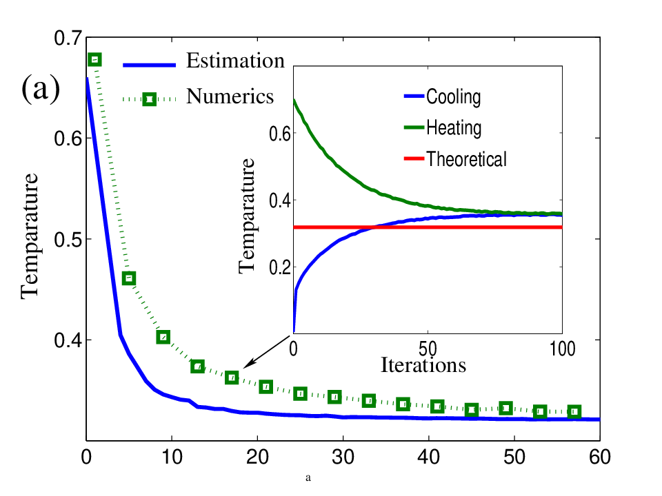
We first considered the ideal case with $k_{c}\to\infty$. As is shown in Fig. 1(a) the effective temperature of the detector changes gradually until it reaches a final steady state after $n\sim 100$ repetitions. The temperature is slightly higher then the value of $T_{U}$ since the finite decoupling time and the final coupling strength increas the average final energy of the steady state. By increasing $\gamma$ we can get closer to the theoretical value of $T_{U}$. In Fig. 1(b) the final temperature is plotted for various values of the detector energy gaps. As can be seen the temperature remains unchanged in agreement with a thermal distribution, up to fluctuations of $\Delta T/T\sim 1\%$. The corrections observed here is due to the finiteness of the number of modes and the interaction time.

Next we extended the analysis to the full problem with a finite cutoff scale $\omega_{c}=c_{s}k_{c}$ which corresponds in a realistic BEC to more than $10kHz$, and is two orders of magnitude larger than the atomdot’s minimal energy gap, which is limited by the fluctuations of the laser. There are two types of corrections. The first type is due to the changing dispersion relation; since the phase in the transition amplitude is now given by, $e^{\pm i\omega_{d}t}e^{i(kx-\omega t)}=e^{\pm i\omega_{d}t}e^{i(ckt-cke^{-at}/a-\omega(k)t)}=e^{\pm i\omega_{d}t}e^{i(\left(ck-\omega(k)\right)t-cke^{-at}/a)}$, the detector’s energy gap is corrected by $ck-\omega(k)$, which is always a negative quantity. For certain modes the effective detector gap can vanish, which implies a divergence in the resulting partial excitation probability. For higher modes the temperature can then becomes negative, which causes a gradual population inversion since $P_{\pm}=\frac{2\pi c_{s}}{\pm\omega_{d}a}\frac{1}{e^{\pm 2\pi\omega_{d}c/a}-1},$ the ratio for large frequency tends to unity. This cutoff effect would be felt once $\omega_{d}=ck-\omega(k)$, which is smaller than the field cutoff. The second type of correction comes from the modified momentum dependence of mode functions $u_{k}$ and $v_{k}$. As $k$ increases $v_{k}$ decreases to zero, hence for $T>t_{c}(k_{c})$ the temperature starts decreasing.

In order to observe the Unruh effect, we can reduce the effects of the above ‘ultra-high’ frequency corrections by selecting a sufficiently short time scale. Fig. 2 displays the resulting final temperature for a numerical computation which includes all Boguliubov’s theory corrections. The expected thermalization effect can be observed but due to the shorter interaction time requires a slightly higher number of repetitions, $n\sim 300$. In order to decrease the number of repetitions the initial state can be chosen at the vicinity of the final temperature. To avoid finite temperature corrections, we need to have the phonon number in the relevant interacting modes to be smaller then 1. For a BEC temperature of $50nk$ this requires a gap energy on the order of $1kHz$.

Another interesting experimental possibility is to simulate the effect of circular acceleration [3, 15]. Unlike the ideal Unruh effect, here the accelerating detector sees the vacuum as excited but usually is not thermalized, i.e., it’s final temperature depends on the energy gap. The advantage of this setup is that the detector does not have to satisfy relativistic equations and thus no special path is needed. Moreover, in the limit where the frequency of rotation is much smaller than the energy gap, the interaction is effectively non-zero only with a finite band of frequencies. Consequently the effect can be insensitive to the cutoff. The limit of $v\approx c$ is especially interesting since the temperature divergence and the detector becomes thermalized, making this regime ideal for experiment. The rotation of the detector could be realized either using dipole traps[16] or optical lattices[17], in both setups the speed of rotation could reach the speed of sound. This makes the circular variant simpler to manifest than the linear one. Fig.3 displays the numeric results for a thermalization effect of a circulating atomic quantum dot.

We remark that a fuller relativistic-like realization, can be done as follows: we consider the condensate coupled to the AD as in Eq. (2), but choose the detuning $\delta=0$. Using Boguliubov’s expansion we then obtain the Hamiltonian $H_{r}\approx\Omega(t)[\phi(d+d^{\dagger})+(d-d^{\dagger})\sum_{k}u_{k}(b_{k}-b_{k}^{\dagger})]\equiv\Omega H^{\prime}$, where $k<k_{c}$ was assumed. The first term represents the free detector Hamiltonian (energy levels have become superpositions of number states) and the second term the interaction with the field. The idea is then to use the common factor $\Omega(t)$ and modify the laser intensity so that $\Omega(t)\propto{d\tau\over dt}={1\over\sqrt{t^{2}+c_{s}^{2}/a^{2}}}$. Upon integration $\int H_{r}dt=\int H^{\prime}d\tau$, hence this recovers the Unruh effect for a uniform-like accelerating trajectory.

In conclusion, we found that a moving AD or an atomic lattice in a condensate can be used to detect acceleration radiation effects that are analogous to the Unruh effect. Our results indicate that the measurability of such effects is within reach of current methods. We hope that the analogy that we are making may be also useful the other way around; that is to interpret what happens when one moves a particle in a condensate with some acceleration.

A. R. and M.B. P. acknowledge support of the European Commission under the Integrated Project (QAP), the Royal Society and EPSRC QIP-IRC. A. R. thanks M. khudaverdyan for many useful discussions. B. R. and J.I. C. acknowledge support by GIF Grant no. I-857.

References

- [1] W.G. Unruh. Phys. Rev. D, 14,870 (1976).
- [2] N.D. Birrell and P.C.W. Davies. Quantum fields in curved space. Cambridge University Press, Cambridge, United Kingdom, 1986.
- [3] J.S. Bell and J.M Leinaas. Nuc. Phys, B 212, 131 (1983).
- [4] J. Rogers, Phys. Rev. Lett. 61, 2113 (1988).
- [5] P. Chen and T. Tajima . Phys. Rev. Letters. 83, 256 (1999).
- [6] M.O. Scully et al.. Phys. Rev. Letters. 91, 243004 (2006).
- [7] P. O. Fedichev and Uwe R. Fischer. Phys. Rev. Letters. 91, 240407 (2003).
- [8] L. J. Garay, J. R. Anglin, J. I. Cirac and and P. Zoller. Phys. Rev. Letters. 85, 4643 (2000).
- [9] P. M. Alsing, J. P. Dowling, and G. J. Milburn. Phys. Rev. Letters. 94, 220401 (2005).
- [10] H.C. Rosu. Grav.Cosmol. 7, 1 (2001).
- [11] A. Recati et al.. Phys. Rev. Lett. 94, 040404 (2005).
- [12] The initial vacuum state is also effectively displaced, however within the relevant parameters this effect can be ignored.
- [13] P. M. Alsing and P. W. Milonni. Am. J. Phys. 72, 1524 (2004).
- [14] R. B. Diener, B. Wu, M. G. Raizen and Q. Niu Phys. Rev. Letters. 89, 070401 (2002).
- [15] O. Levin, Y. Peleg, and A Peres. J. Phys. A: Math. Gen. 26, 3001 (1993).
- [16] J. Beugnon et al.. arXiv:0705.0312.
- [17] S. Tung, V. Schweikhard and E. A. Cornell. cond-mat/0607697.