On the Magnitude of Dark Energy Voids and Overdensities
Abstract
We investigate the clustering of dark energy within matter overdensities and voids. In particular, we derive an analytical expression for the dark energy density perturbations, which is valid both in the linear, quasi-linear and fully non-linear regime of structure formation. We also investigate the possibility of detecting such dark energy clustering through the ISW effect. In the case of uncoupled quintessence models, if the mass of the field is of order the Hubble scale today or smaller, dark energy fluctuations are always small compared to the matter density contrast. Even when the matter perturbations enter the non-linear regime, the dark energy perturbations remain linear. We find that virialised clusters and voids correspond to local overdensities in dark energy, with for voids, for super-voids and for a typical virialised cluster. If voids with radii of exist within the visible Universe then may be as large as . Linear overdensities of matter and super-clusters generally correspond to local voids in dark energy; for a typical super-cluster: . The approach taken in this work could be straightforwardly extended to study the clustering of more general dark energy models.
Subject headings
Cosmology: Theory, miscellaneous. Relativity. Galaxies: general, Large scale structure of the universe.I. Introduction
It has been almost a decade since observations of Type Ia supernovae (SNe Ia) were first found to support the notion that our universe is currently undergoing a phase of accelerated expansion (Riess et al. 1998; Perlmutter et al. 1999). Since that time, evidence in favour of this accelerated expansion has strengthened significantly as the result of further SNe Ia observations (Riess et al. 2004; Riess et al. 2006a; Riess et al. 2006b; Wood-Vasey et al. 2007), improved measurements of the cosmic microwave background (CMB) (Spergel et al. 2003; Spergel et al. 2007) and surveys of large scale structure (LSS) (Adelman-McCarthy et al. 2006; Tegmark et al. 2006). The precise cause of this late-time acceleration, however, remains unknown.
If general relativity is accurate on astrophysical scales, then the assumptions of large-scale homogeneity and isotropy require that the agent responsible for the universe’s acceleration, dubbed ‘dark energy’, behave cosmologically as a fluid with negative pressure. The standard model of particle physics predicts only one such fluid: the vacuum energy, or cosmological constant, for which the pressure, , is always equal to minus the energy density, . However, if the vacuum energy density is indeed non-zero then it is generally expected to be of the order of , where is the Planck-mass. This is some orders of magnitude larger than the observed dark energy density. A number of proposals have therefore been made in the literature for models in which dark energy is dynamical and associated with some new form of energy (Wetterich 1988; Peebles & Ratra 1988). In these models, the present small size of the effective cosmological constant is by-product of the age of Universe. The acceleration of the Universe might alternatively be explained by modifying General Relativity rather than postulating a new form of energy (Dvali, Gabadadze & Porrati 2000; Amarzguioui et al. 2006; Nojiri & Odintsov 2003; Capozziello, Cardone & Troisi 2005; Koivisto & Mota 2007a; Koivisto & Mota 2007b, see). It also been suggested that the Universe is not accelerating at all, but that a large local inhomogeneity prevents the SNe Ia data from being correctly interpreted in terms of a homogeneous and isotropic cosmological model (Kolb Matarrese & Riotto 2006; Moffat 2006). This said, dynamical dark energy (hereafter DDE) is by far the most popular candidate to explain the current astronomical data. In the simplest DDE models, known as quintessence, dark energy is associated with the energy density of a scalar field with a canonical kinetic structure.
If dark energy does indeed exist then astronomical observations presently provide us with only hints as to its nature. We know that today it represents about of the total energy density of the Universe, and that its equation of state (EoS) parameter, , is fairly close to : for , (Riess et al. 2006a). Furthermore, if matter dominates the expansion of the Universe for then (Riess et al. 2006a). Hence, dark energy has negative pressure at higher redshifts with a confidence. These bounds on are entirely consistent with a pure cosmological constant. Whilst detecting either or would rule out a cosmological constant, in many DDE models significant deviations from only occur at early times and as such would be difficult to detect. The late time, background cosmology predicted by many DDE models is therefore very similar to that of a universe with a true cosmological constant.
DDE models generally cease to mimic a cosmological constant in inhomogeneous backgrounds or when one considers cosmological perturbation theory. In particular, a number of authors have studied the effect of DDE on the formation of large scale structure (Corasaniti, Giannantonio & Melchiorri 2005; Hannestad & Mortsell 2002; Brookfield et al. 2006b; Doran, Robbers & Wetterich 2007). In the vast majority of these works the energy density of dark energy is taken to be homogeneous i.e. it is assumed that DDE does not cluster. The extent to which this assumption of homogeneity is valid has been the subject of some interest and much debate in the literature. In an inhomogeneous background, the DDE energy density and EoS parameter should exhibit some spatial variations. The key issue of how large these variations should be is however far from settled, particularly when the matter perturbation goes non-linear (Maor & Lahav 2005; Mota & van de Bruck 2004; Linder & White 2005; Bartelmann, Doran & Wetterich 2005; Nunes & Mota 2006; Abramo et al. 2007). In this paper we attempt to settle this issue for uncoupled quintessence models by deriving an analytical expression for the dark energy contrast, , in by presence of a matter perturbation. Importantly, we do not constrain the matter perturbation to be small (i.e. linear).
Clustering of DDE over scales smaller than about has been the subject of a number of recent articles (Caimmi 2007; Balaguera-Antolínez, Mota & Nowakowski 2006; Mainini 2005; Percival 2005; Wang 2006; Nunes, da Silva & Aghanim 2005; Balaguera-Antolínez, Mota & Nowakowski 2007). Most attention has been focussed on models in which the DDE couples to baryonic and/or dark matter since DDE clustering is expected to be strongest in such theories (Amendola 2000; Brookfield et al. 2006a; Manera & Mota 2006; Pettorino, Baccigalupi & Mangano 2005). In other works, a more phenomenological approach has been taken and the observables associated with DDE clustering have been parametrized. In particular, it has been shown that inhomogeneities in dark energy could produce detectable signatures on the CMB (Weller & Lewis 2003; Koivisto & Mota 2006).
Recently, Dutta & Maor 2007 considered the growth of spatial DDE perturbations in the absence of any matter coupling. They considered only those circumstances where both the density contrast of matter, , and that of the DDE, , were small enough to be treated as a linearized perturbations about a homogeneous and isotropic cosmological background. They studied the simplest class of quintessence models where dark energy is associated with the slow-roll of a scalar field down a potential ; is minimally coupled to gravity. The authors linearized the full field equations for , the matter and the metric and solved the resulting system numerically. Intriguingly they found that, at late times, a local overdensity of matter corresponded to a local under-density, or void, of dark energy. Conversely, a void in the matter was seen to produce a local DDE overdensity. Although the DDE density contrast, , is initially very small compared to the matter density contrast, , they found that, when , . was also observed to be growing more quickly than at late times. Their results suggest that DDE clustering may induce a positive correction to the value of of more than at the centre of an inhomogeneity with properties similar to that of the local supercluster (hereafter LSC). If accurate, the results of Dutta & Maor 2007 imply that any deviations from would be significantly amplified by the presence of a local overdensity of matter. Furthermore, they suggest that DDE clustering might be relatively strong when the matter perturbation goes non-linear.
Dutta & Maor 2007 studied DDE clustering when the matter perturbation is growing in the linear regime, which is only accurate when . They considered the evolution for a cluster of matter with initial density profile (at ) of where and with being the initial value of the Hubble parameter. However, in the absence of any DDE, the linear approximation would generally cease to be accurate when ; additionally the perturbation would be expected to turnaround when and virialise when . It is therefore far from clear whether or not the sharp late-time growth in found by Dutta & Maor 2007 is indeed a physical effect, or just a result of using linearized field equations outside of realm in which they are valid. Although one might well expect there exist some mapping between the linear and non-linear regimes as it happens in an Einstein-de Sitter Universe.
In this paper we investigate a similar problem to that considered by Dutta & Maor 2007, i.e. the clustering of uncoupled quintessence on sub-horizon scales. There are, however, two important differences between our approach to this problem and the one taken by Dutta & Maor 2007:
- 1.
Firstly, we do not use numerical simulations but instead use the method of matched asymptotic expansions (MAEs) to develop a analytical approximation to .
- 2.
Secondly, we do not require the density contrast of the matter perturbation, , to be small. Indeed, our analysis and results remain valid even after the virialisation of the matter overdensity.
Our approximation for is accurate provided that is only non-linear () on sub-horizon scales. This provision is consistent with observations. For simplicity we take the matter perturbation to be spherical symmetric. We also require that gravity is suitably weak whenever the inhomogeneity is non-linear i.e. . We restate these requirements in a rigorous fashion later, however they are essentially equivalent to the statement that gravity is approximately Newtonian over scales smaller than . Since DDE clustering in the linear regime has been dealt with in great detail by Dutta & Maor 2007, our main focus in this paper is on what occurs when the matter perturbation goes non-linear.
This paper is organized as follows: in Section II we describe our model for an inhomogeneous spacetime and the DDE. We state the equations that must be satisfied by the metric quantities and the dark energy scalar field . In Section III we introduce the method of matched asymptotic expansions (MAEs). This method relies the existence of locally small parameters, and we state what these are for our model and interpret them physically. We also note what constraints the smallness of these parameters places upon our analysis. In Section IV we apply the method of MAEs to the evolution of dynamical dark energy perturbations. We derive a simple equation for the DDE density contrast, , in terms of the peculiar velocity of matter particles, , and the matter density contrast, . Importantly this equation is equally as valid for (‘the non-linear regime’) as it is when (‘the linear regime’). In Section V we use our results to study the evolution of in the linear (), quasi-linear () and fully non-linear () regimes. We compare our analytical results with those found numerically in the linear regime by Dutta & Maor 2007. In Section VI we consider the spatial profile of the DDE density contrast for realistic astrophysical inhomogeneities such as voids, supervoids, clusters and superclusters. We conclude in Section VII with a discussion of our results and their observational implications. We also note how our analysis might be extended to include even more general DDE models.
Throughout the paper we use units where .
II. The Model
II.1. Geometrical Set-Up
Our aim in this paper is to derive an expression for the DDE density contrast, , inside an over-density, or under-density, of matter. Henceforth we use to represent the energy density of a component . We are particularly interested in those cases where the matter perturbation is non-linear i.e. . Although we aim to remain suitably general in our treatment of the density perturbation, we do make the following simplifying assumptions:
- •
We assume spherical symmetry. We briefly discuss the extent to which the relaxation of this assumption would affect our results in Section VII below, and conclude that the qualitative nature of our findings would be unaffected.
- •
We define a ‘physical radial coordinate’, , by the requirement that a spherical surface with physical radius has surface area . We assume that all curvature invariants are regular at i.e. we do not consider those cases in which there is a central black hole. We argue below, however, that our results are still accurate even when there is a central black-hole, provided they are only applied at radii that are large compared to the Schwarzschild radius of the black hole.
- •
Finally we assume that for radii smaller than some gravity is suitably weak in the inhomogeneous region; is the Hubble parameter of the background spacetime. We define what we mean by weak rigorously in Section III. For radii , we require that the matter density contrast is . This assumption holds for most realistic models of collapsing overdensities provided that the radius the overdense region is less than about .
II.2. Einstein’s Equations
We take the matter content of the Universe to be a mix of irrotational dust and dynamical dark energy, which is described by a scalar field . For simplicity we restrict ourselves to considering only spherically symmetric spacetimes for which the most general line element in comoving coordinates is:
We make the definitions and . This coordinate choice is unique up to , and . With these definitions the 2-spheres have surface area , and in this sense represents the ‘physical radial coordinate’. The energy-momentum tensor of pressureless dust is given by
and the energy-momentum tensor of the scalar field, , is
The Einstein equations for this metric read:
| (1) |
where . The -component of Eq. (1) gives:
| (2) | |||||
and the -component of the Einstein equations is:
| (3) |
The -component of Eq. (1) reads:
| (4) | |||||
¿From , it follows that:
| (5) |
where is an arbitrary constant of integration. If we define so that for some , then where is the mass inside a shell of radius at .
¿From one obtains:
| (6) |
Eq. (6) is subject to the boundary conditions: at , and , where is the solution of Eq. (6) in the cosmological background. We make the following definitions:
where is defined by . We also define:
Integrating Eqs. (2) and (4) and using Eqs. (3) and (6) we find that
| (7) | |||||
and
| (8) | |||
As we must recover the FRW background cosmology which implies:
where is an arbitrary time, is the scale factor of the FRW background, and is the curvature of the background. In line with current observations, and because it greatly simplifies the calculations, we take the cosmological background to be flat and set . We do not attempt to solve the Einstein or DDE equations exactly, but instead we develop asymptotic approximations to the true solutions which are accurate so long as a number of parameters, which we define and interpret below, remain small.
III. Small Parameters and the Matched Asymptotic Expansions.
One can think of the small parameters approach and the matched asymptotic expansions as an expansion in the Newtonian potential. Although it is perhaps fairer to say that is closest to the context of General Relativity. The differences are not obvious at leading order but at next to leading order one will see that what appears in the equation for the acceleration is not necessarily what one would expect to appear in the Non-relativistic regime.
As stated above in Section II.1, we require that gravity is ‘suitably weak’ inside the density perturbation. By suitably weak we mean that
where
Physically is the velocity of a particle of dust in coordinates, where is the physical radial coordinate, and is the velocity that such a particle would have in the cosmological background. The small parameter is therefore the peculiar velocity of a matter particle with respect to the cosmological background. Recall that we use units where , hence the first expression above is in fact the dimensionless quantity . Our assumption requires that whenever , we have . This condition is equivalent to requiring that the mean matter density contrast, , inside the sphere with radius or greater, is small enough that it may be treated as a linear perturbation about the cosmological background. The mean matter perturbation is however allowed to be non-linear, , when provided . We also define
We require . This again require that only when i.e. the matter perturbation is only non-linear on sub-horizon scales. We note that , and so generally provided .
In what follows we assume that and are small everywhere. These assumptions can be checked once one specifies initial conditions for the matter overdensity, but they generally hold very well whenever the scale of the inhomogeneous region is .
We now define two over-lapping regions which we shall refer to as the interior and the exterior.

III.1. The Interior Region
The interior region is defined by
We define the inner limit of a quantity to be . The inner limit can be imagined as the limit in which the cosmological background density of matter is taken to zero, and the cosmological horizon is taken to infinity. In the interior we construct asymptotic approximations to quantities in the limit . We also expand in and . We refer to this as the inner approximation.
III.2. The Exterior Region
In the exterior region, spacetime is required to be homogeneous and isotropic at leading order. In other words, the matter perturbation must be linear in the exterior:
From the form of , it is clear that implies . We define the exterior limit of a quantity to be . As in the interior limit we also expand in and . We construct asymptotic approximations to quantities in the exterior region in this exterior limit and refer to them as the outer approximations.
III.3. Matching and the Intermediate Region
We are primarily concerned with the behaviour of the DDE in the interior region. In Section IV, we find the inner approximation to by solving Eq. (6) order by order in the interior limit. We cannot, however, apply both of the boundary conditions on directly to the inner approximation. This is because the condition must be applied at , a point that is very clearly in the exterior and not in the interior region. As a result, the inner approximation will contain ambiguous constants of integration. Fortunately, this ambiguity can be lifted by matching the inner and outer approximations to if there exists some intermediate region where both approximations are simultaneously valid. This matching of the inner approximation to the outer one is referred to as the method of matched asymptotic expansions (MAEs). It relies on the fact that, in any given region, the asymptotic expansion of a quantity is unique (Hinch 1991, for a proof see). Thus if the inner and outer approximations of are both valid in the intermediate region, they must be equal in that region. For the method of MAE to be applicable we must, of course, require that an intermediate region exists. A necessary condition for an intermediate region to exist is that for some range of :
This becomes a necessary and sufficient condition if the only boundary of the interior region is in the exterior one, and vice versa (see Figure 1 for an illustration). If the scale of the inhomogeneity, , is taken to be the largest value of for which , and then then an intermediate region generally exists provided that .
In resume, in this section we have considered spherically symmetric backgrounds and far from black hole horizons. We have basically performed an expansion in the Newtonian potential at leading order, at least as far as the evolution of scalar field perturbations are concerned. Notice, however, that this method can be straightforwardly extended to allow for deviations from spherical symmetry (Shaw & Barrow 2006a; Shaw & Barrow 2006b; Shaw & Barrow 2006c).
To be clear, we should point out that the expansion in and , which is a lot like expanding in the Newtonian potential, is not really the key to our method. That is just a simplification. The key is that we take: in the interior region and in the exterior region. That is, everything is linear in those two regions. We then assume that there is an intermediate region where both of these conditions hold. Which implies that in the intermediate region: and . So the assumption that everywhere ensures that we have an intermediate region. We could in fact relax this but the calculations would become more difficult: often still doable, but in almost all physically interesting cases totally unnecessary. For instance the relaxation to and , is very straightforward and allows one to go all the way up to a black hole horizon (Shaw & Barrow 2006a; Shaw & Barrow 2006b; Shaw & Barrow 2006c).
IV. Evolution of Dynamical Dark Energy Perturbations
In this section we find an asymptotic approximation to the DDE density contrast, . The discussion is fairly technical, and readers more interested in the results than the machinery used to derive them may prefer to focus on the statement, discussion and application of our results in Section IV.3 and following.
The DDE is described by the field which satisfies:
We solve this equation by constructing an asymptotic approximation to in the small parameter . We write:
where . Before solving for , we make the dependence of the metric on explicit by transforming to a new radial coordinate, , where is the scale factor of the Friedmann-Robertson-Walker (FRW) cosmological background. In coordinates the metric is:
| (9) | |||||
Consider in this metric:
where is evaluated at constant as opposed to constant or and is thus given by Eq. (3). It follows that satisfies:
| (10) | |||||
We now solve for in both the interior and exterior regions.
IV.1. Inner Approximation
We note that , and that , so that
In many cases is small enough so that
and so that evolves over cosmological time-scales. In these cases it is clear that:
and so this term can be dropped at leading order. Although it will often be the case that we do not have to require such a strong assumption in order to justify ignoring the effect of the potential to leading order in the interior approximation. Instead, we make the far weaker assumption that:
| (11) |
A physically-viable DDE theory for which this requirement does not hold would be difficult to construct. For instance, if this condition did not hold then even if, at one instant, or smaller, as must be required for to evolve over cosmological time scales, shortly afterwards small changes in would cause to grow to be many orders of magnitude greater than . This would result in evolving over time-scales that are much shorter than the Hubble time. The only DDE theories that we can imagine that could accommodate this and still be compatible with observations would involve being held almost completely fixed at a minimum of , in which case the DDE would be almost entirely indistinguishable from a cosmological constant.
To leading order in the interior, we would actually be justified in setting as . However, since it might not be completely clear that these terms may be ignored, and because we can solve the equation without having to ignore them, we continue to include them.
We define and , and note that , so that:
| (12) |
which has as a solution
| (13) | |||||
where and ; and represent waves in the scalar field and we discuss them further momentarily. To go further, we make the following reasonable assumptions about the behaviour of . We assume that there exists some , in the interior region, such that for in the interior region, decreases faster than as ; then decreases faster than for . This assumption ensures that dominant contributions to the integral in Eq. (13) comes from values of that are well inside the interior region. Note that generally varies over conformal times-scales of order and . Provided that is not momentarily zero, these scales are much larger than so we can Taylor expand as
where the neglected terms are times . After some algebra and integration we then arrive at:
| (14) |
where the previous assumption relating to the Taylor expansion of can be seen to be equivalent to the statement that . This assumption will generally break down if there is some initial instant, say, when . At however, is equivalent to , which is certainly the case in the interior region.
Generally, the functions and are related to the initial conditions on . Because we have required our analysis will break down at early times since generally as . As a result, we cannot generally determine and by simply specifying some initial conditions on, at say, and applying them to the interior approximation since the interior approximation by not be valid when . The requirement that can however be applied to the interior approximation to give . To the order at which we work, itself should be fixed by matching to the outer approximation.
IV.2. Exterior Solution and Matching
In order for we must have as . In the exterior region, spacetime is FRW to leading order in and , and the equation describing for the leading order behaviour of reads:
| (15) | |||||
where . Solving this equation is far from straightforward. Fortunately, however, our main interest in not in how behaves in the exterior region but in interior region where the perturbation in the matter density can be non-linear, and so it is not necessary to solve Eq. (15) in the exterior region so long as we know how its solutions behave in some intermediate region where . We require that as the matter perturbation is removed i.e. . We have also required that drop off faster than for where is in the interior region i.e. . In this intermediate region, the solutions of Eq. (15) for which as have the following form:
| (16) | |||||
where or greater. We have assumed that is larger compared to any initial instant when one one or more of , or hold. With these assumptions, matching to the interior region gives:
and
We have required drop off of means that, to leading order, we can set . This implies that the is sub-leading order in the interior approximation and so may be neglected.
Thus to leading order in the interior region we find:
Where is the peculiar radial velocity of the matter particles relative to the expansion of the background Universe. This approximation is valid in the interior region at late times compared to any initial instance when and/or which is equivalent to . Note that, to this order, the surfaces of constant are surfaces of constant:
We use this asymptotic approximation for to evaluate the DDE density contrast on surfaces of constant in the matter rest frame. In the rest frame of the matter particles:
and the local inhomogeneity in is therefore:
| (17) | |||||
The corrections terms are times smaller than the leading order term. Since we have
is the acceleration of the matter particles in coordinates. Eq. (II.2) gives:
where is the mass contrast at time inside the sphere with physical radius .
IV.3. Discussion
In this section we found that the DDE density contrast can be expressed, to leading order, in terms of the radial peculiar velocity, , the mean density contrast, and the unperturbed DDE equation of state parameter :
| (18) | |||||
This expression for is our main result and it is valid for both linear and non-linear sub-horizon matter perturbations. In order to evaluate the above expression, one must simply specify the peculiar velocity, , of the matter particles and the matter density contrast . This exterior is valid in the interior region at late times compared to any initial instance when and/or i.e. .
Note that and will depend on the mass of the field , so in that sense, equation (18) is not completely model independent. However, all the model dependent terms come from the homogeneous and isotropic background cosmology. So the expression for is model independent provided . Which is true if and as assumed.
The key point is that large deviations in from the prediction using a LCDM background could only occur if and were predicted to change by an order of magnitude or more. As far as we know, however, structure formation is compatible with LCDM over the scales of clusters and so it seems unlikely that such large deviations occur.
As we shall see below the DDE perturbation is generally small compared to the matter perturbation, so to leading order one may neglect any DDE perturbations when evaluating and .
It is interesting to note that the sign of depends on the relative magnitudes of and : From equation (18) one deduces that the formation of local overdensities or local voids of dark energy arise from two competing effects:
- •
The Drag effect: associated with deviations from . If one has an overdense region, then it expands more slowly. In agreement with Dutta & Maor 2007, we find this drag effect to produce a local underdensity of dark energy.
- •
The Pull effect: associated with deviations from . An overdensity of matter pulls the dark energy (and everything else) towards it. So matter and fields tend to clump around it. As a result, the pull effect means that an overdensity of matter creates an overdensity of DE.
So there is one effect that pulls the dark energy in and another that pushes it out. As we will see, in the linear regime the drag effect grows more quickly than the pull effect, so one gets a dark energy void. The onset of non-linear structure formation, however, causes to reach a maximum and then to tend to at late times, whereas just keeps on growing. So the pull effect dominates at late times, so one ends up with an overdensity of dark energy.
We have assumed above that the mass of the DDE scalar field is small compared to the inverse length scale of the cluster. Provided this is in uncoupled DDE theories is independent of the details of theory describing the dark energy.
In the next section we use Eq. (18) to evaluate in both the linear and non-linear regimes. We find that , where is the radial scale of the cluster, and is the mean matter density contrast in .
V. Clustering of Dynamical Dark Energy
V.1. Dynamical Dark Energy Clustering in the Linear Regime
Although one of our main aim in this work was to study DDE clustering in the non-linear regime, our analysis is also perfectly valid in the linear regime, i.e. when , provided that the matter inhomogeneity is sub-horizon at the instant when we wish to evaluate . We found above that is given by Eq. (18). In the linear regime , and so the term proportional in Eq. (18) is small compared to the other two terms and should be neglected. is the matter density contrast, and we define to be its Fourier transform. In the linear regime (in comoving-coordinates):
and so:
where and is the Fourier transform of . We recognize that where is the leading order perturbation to the Newtonian potential. is given by:
The Fourier transform of is therefore: , and the Fourier transform of the DDE density contrast, , in the linear regime is given by:
| (19) |
where
| (20) |


Motivated by observations, we assume to be small at late times, and to be small at early times. To a first approximation then we approximate by its CDM value. At late times a very good approximation to in the CDM model is (Peebles 1980; Lahav et al. 1991). Note that corrections to this fitting formulae occur for quintessence-like models (Wang & Steinhardt 1998). However, these are generally too small to greatly affect our results. Hence we take the CDM expression for simplicity. Even when it is not acceptable to approximate by its CDM, we do not expect this approximation to greatly alter the qualitative nature of our results or the order of magnitude of .
Transforming back into real space we have:
| (21) |
Our expression for is independent of the mass of . This is because we have assumed that in the linear regime and that the matter perturbation is small compared with . The mass of the scalar field therefore has only a negligible effect on the scales over DDE clustering occurs. It is clear that the sign of is the same as the sign of . At late times , and so a linear local overdensity of matter () corresponds to a DDE void. Similarly, there is a DDE overdensity at late times (in the linear regime) if there is a local void of matter. If an initial mean density perturbation begins to collapse at when , and we have:
| (22) | |||||
and so
Our expression for was derived under the assumption that . As result it will break down as we approach . More precisely, we find that our approximation is valid at for i.e. where is the initial value of and is the initial value of . ¿From this expression we can see that a matter overdensity corresponds initially to a DDE overdensity (), however this DDE overdensity becomes a DDE void at some , and for . We see that is given by:
where we have taken . If , which should be a good approximation for , we have . For this analysis to be valid we must have which with holds . For inhomogeneities that are larger than this at we do not expect to be an accurate approximation to the redshift when the DDE density contrast changes sign.
Note that does not depend on the size of the inhomogeneity, although, of course, we must have for our analysis to be valid, which implies that at , .
If exactly then at late times. If , then grows likes:
at late times in the linear regime. This implies that tends to a constant in the linear regime if , and is growing for . At late times in the linear regime then: . If we take today then is predicted to grow faster than when . Dutta & Maor 2007 also found that at late times in the linear regime grows faster than . This is behaviour were to continue into the non-linear regime it would, of course, imply that would ultimately grow to be very large and indeed dominate over . As we show in this paper, however, before this can happen the matter perturbation goes non-linear and this slows the growth of .
We conclude our analysis of the linear regime by noting that Eq. (21) implies that at late times:
| (23) | |||||
where is defined the smallest value of for which , and depends on the precise form of .
We have shown that in the linear regime at the centre of the inhomogeneity is always smaller than by a factor of about ; is roughly equal to the physical size of the inhomogeneity as a fraction of the horizon size. If the initial density perturbation is Gaussian i.e.
then
and:
at late times.
We plot the evolution of and for a Gaussian initial matter density perturbation in the linear regime in Figure 2. We have assumed that at , and , which corresponds to and and today i.e. . For this choice of inhomogeneity, our approximation for is only good for . Just as Dutta & Maor 2007 saw in their numerical simulations, we find that close to , . It then becomes negative, and at late times it continues to grow more negative, and it appears as if it might overtake at some point in the future. However, as we shall show below, this does not occur and remains small at all times. Note that the apparent increase in at early times is due in part to fact that our approximation breaks down as one approaches . If one wishes to study the evolution of all the way back to , the numerical approach taken by Dutta & Maor 2007 provides accurate results. Our real focus in this work is, however, not on what occurs at very early times in the linear regime, but how the DDE density contrast evolves when the matter inhomogeneity goes non-linear. We consider this below.
V.2. Dynamical Dark Energy Clustering in the Quasi-Linear Regime
We begin our investigation of how evolves when the matter perturbation exits the linear regime by considering a matter perturbation that is in the weakly non-linear or quasi-linear regime i.e. . Eqs.(3) and (4) give . We suppose that at some initial time, , and . is then the mass inside the shell with radius at . We write:
is interpreted as the initial mean matter density contrast. In the full non-linear regime, which we consider in the next subsection, we are only able to evaluate and hence, via Eq. (18), , analytically in a matter-dominated background (). In many cases of interest, however, , e.g. superclusters and voids. Although the linear approximation fails for such objects, a good leading approximation to the true mean density contrast of matter, , in the range, is given by:
where is the linear mean density contrast. This approximation improves as and is exact for . When this approximation holds we say that we are in the quasi-linear regime.
In this section we find for inhomogeneities in the quasi-linear regime. We are again assuming that any deviations from the CDM model for structure formation due the background DDE evolution are sub-leading order i.e. is small. If this is not the case then our expression for in terms of and is still valid, but the evolution of and would change; even still the order of magnitude of would not be greatly effected.


The peculiar velocity, , is related to thus:
where, as above, at late times. In the quasi-linear regime the physical radius, , of a shell with mass is given by:
| (24) | |||||
Using Eq. (18), we find that the dark energy density contrast, , in the quasi-linear regime is well approximated by where:
| (25) | |||


For , the first term in Eq. (25) is negative definite for all positive values of for which the quasi-linear approximation holds () and positive definite for . The second term in Eq. (25) is clearly positive definite but vanishes at . The relative magnitude of the two terms depends on the choice of initial density profile. However, at it is clear that an overdensity of matter, , corresponds to a dark energy void, . Similarly, a void of matter corresponds to a local DDE overdensity at . In Figures 3 and 4 respectively show the evolution of and at for a typical supercluster and a typical void. For both the supercluster and the void we assume an initial density contrast profile that is flat for and drops as for . We take the initial instant to be in the far past i.e. . The supercluster is taken today to have a central density contrast of and to corresponds to a physical radius of , which are appropriate for an object such as the local super-cluster. For the void we take typical values of today and . In each case we have taken . It is clear that in both cases grows faster than , however the DDE density contrast remains much smaller than at all times. Note that evolves monotonically for objects in both the linear and quasi-linear regimes.
V.3. Dynamical Dark Energy Clustering in the Non-Linear Regime
The quasi-linear approximation to is valid for , however it breaks down for large positive values of the matter density contrast, . To go further we evaluate in the fully non-linear regime. To do this we need to calculate both the evolution of the peculiar velocity, , and that of the mean density contrast mass contrast, . The non-linear evolution of the matter overdensity is significantly more simple to calculate analytically in a matter dominated Universe (). Fortunately, when the matter density contrast is large today , the evolution of both and in the inhomogeneous region are well-approximated by the solution. This is because the epoch of dark energy domination begins sometime after the cluster has turned around.

If , we are effectively dealing with a Tolman-Bondi (Tolman 1934; Bondi 1947) background at leading order. We therefore have analytical solutions for and in terms of and a parameter :
| (26) | |||
| (27) |
where
| (28) | |||||
and
We assume that at early times, , . These solutions then provide an excellent approximation to the true early time evolution of the inhomogeneity. These solutions also provide an good approximation at late times, provided we are dealing with an overdensity of matter that turns around prior to the onset of dark energy domination ( today). Assuming that we are dealing with such an overdensity, we find:
| (29) | |||||
When the background is matter-dominated, and . In the non-linear regime , and terms proportional to in the above expression can be dropped.
We have so far modelled the matter as being a spherically symmetric, pressureless perfect fluid. This approximation neglects the random motion of the matter particles, and other effects due to the break down of spherical symmetry. These are small prior to turnaround but thereafter act to slow down the collapse of the inhomogeneity. Without any such corrections the matter perturbation would eventually collapse to a point. When these effects are included however the inhomogeneity virialises and relaxes to a steady-state. In a matter-dominated background, each shell of constant ceases to collapse and virialises when its radius, , is about one half of the radius at which it turned around, . N-body simulations suggest that (Hamilton et al. 1991, see).

Since process of virialisation is not accounted for in our matter model, we must account for it in some fashion if we are to make accurate predictions. This is generally done via the rather ad hoc process of manually halting the collapse when each shell reaches its virial radius, ; in this model one takes ; this occur at . Whilst this provides a reasonably good approximation for the magnitude of the density contrast, , the peculiar velocity, , is discontinuous at instant of virialisation (). This ad hoc procedure therefore gives widely inaccurate predictions for the peculiar velocity, (see Figure 5). Since our formula for depends on both and we require a more realistic model for virialisation in the context of spherical collapse. Such an improved model was proposed recently by Shaw & Mota 2007. In this improved spherical collapse model, it is assumed that is a function of i.e. . is still parametrized according to Eq. (26), and it is found that:
where . The function is then fixed so that: Prior to turnaround, when deviations from spherical symmetry are small, . For larger values of (), is chosen so that agrees, under certain reasonable and common assumptions, with the behaviour that is seen in N-body simulations of Hamilton et al. 1991. Shaw & Mota 2007 provide the following fitting formula for :
| (30) |
where . In this model which compares more favourably with the value of suggested by N-body simulations (Hamilton et al. 1991) than the value of that is generally used. In this improved model, is still given by Eq. 18, and for the peculiar velocity is given by:
and the density contrast is given by:
Figure 5 shows as a function of in both the improved spherical collapse model, and the standard one (with virialisation occurring suddenly at ). Note that in the standard spherical collapse model (SCM), continues to grow until , and then drops sharply, whereas in the improved model reaches a maximum when . Note also that the maximum value of predicted by standard SCM is almost five times as large as the maximum value gives by the improved model. Since depends in part on and hence , using the standard SCM instead over the improved model could lead to being over estimated by as much as .
Figure 6 shows , for , as a function of the mean linear density contrast, , in both the improved model and the standard one with virialisation put in by hand. We use our modified spherical collapse model to find the evolution of . We find then that the DDE density contrast in the non-linear regime is given by:
| (31) | |||||
where
When , , and deep in the non-linear regime, when , . In the case we find that the following fitting formula is accurate to within :
| (32) | |||
We note that when , for and is otherwise positive. In a cluster with a core overdensity , is therefore generally positive at i.e. there is DDE overdensity at , whereas for clusters with a core overdensity , there is generally a DDE void around . Even in the deep non-linear regime, the central DDE overdensity is still surrounded by a void, with becoming negative when . We see that , where is the radius of the core of cluster (roughly defined by smallest radius after which decreases faster than ), and is the core density contrast i.e. the density contrast at .


We use Eq. (31) to plot the evolution of in the non-linear regime. For , the matter overdensity in a background with evolves, to a good approximation, according to:
where and . We expect the largest contributions to to come from regions where which implies that the we expect for all . Therefore, using Eq. (31), we approximate:
| (33) | |||||


For simplicity, we take the initial density profile to have a central core with for and for , we take: .
In Figure 7 we plot and for a cluster where today corresponds to a physical radius of , and the mean density contrast in today is . In Figure. 8 we plot and for a smaller but denser cluster with and today. These values are fairly typical of clusters such as Coma which has been estimated to have a mean density contrast of inside a radius of , and a core mean density contrast of about inside a radius of . We can see that in both cases today and that, as expected, it is positive. In both cases, was negative in the past, changing sign when the mean overdensity of the core was . The core in these cases corresponds to the flat part of i.e. . For more general density profiles, the core radius would be taken to correspond to where is the smallest value of for which faster as . In all of the plots we have taken .
We can see that in both cases continues to increase today. This increase is due to the continued collapse of matter onto the collapsed core. At very late times, however, this accretion will cease, and for all . We can see this from Eq. (31). At late times, and assuming minimal accretion: , for some function , and so:
| (34) |
and which implies at late times. It is clear that is smaller than by at a factor of about . In follows that even at late times , as , where .
V.4. Discussion
We have seen that in all regimes (linear, quasi-linear and fully non-linear regimes), the magnitude of DDE density contrast scales as: , where is the radial scale of the cluster, and is the mean matter density contrast in . is roughly defined to be equal to , which is the smallest radius for which first decreases faster than . If an inhomogeneity is sub-horizon when it begins to collapse, we found that shorter after the collapse begins and have the same sign i.e. a matter overdensity equates to a DDE overdensity, and the same for voids. However, a certain time after collapse begins, changes sign. This change of sign is related to the fact that at late times the decaying mode of the matter perturbation is negligible. When this occurs, a mean over density of matter results in a DDE void, and vice versa. Deep in the non-linear regime, when , however, changes sign again. A large mean overdensity of matter then corresponds to an overdensity of dark energy at .
In both the linear and the quasi-linear regimes, increases faster than , although it is always much smaller than . This behaviour was also observed by Dutta & Maor 2007 in their numerical study of the linear regime, and it lead them to wonder whether might grow to be or larger in the non-linear regime. Using our results, we have shown that the onset of non-linear evolution for the matter perturbation slows down the growth of and that at very late times and remains . In the next section we consider the profile of in and around typical astrophysical objects.
VI. Astrophysical Applications
In this section we use our results to evaluate the profile of the DDE density contrast around typical clusters, superclusters and voids of matter. We also investigate the possibility of detecting the dark energy clustering using the Integrated Sachs Wolfe (ISW) effect.
VI.1. Galaxy Clusters


We begin by considering the DDE density contrast in a virialised galaxy cluster with similar properties to the Coma cluster. Navarro, Frenk & White 1997 (hereafter NFW) used high resolution N-body simulations to derive a universal density profile for the dark-matter halos of virialised structures such as galaxies and clusters. The resulting NFW profile is given by:
where defines the scale at which changes from a drop-off to a one, and the characteristic density contrast is given by:
where defines the concentration of the halo, and is roughly the virial radius and is defined to be the largest value of for which the mean density contrast is . The mean density profile, , is then given by:
Even though for , the integrands in Eq. (31) still behave well enough for small for our analysis and our expression for to be valid and applicable. The DDE density contrast in a virialised cluster is given by Eq. (31). We note that since , in the non-linear regime, and depends on only though that, for fixed , .
Geller, Diaferio & Kurtz 1999 studied the mass profile of the Coma galaxy cluster and found that over the entire range of it increased with at the rate predicted by the NFW profile. They found that three different observational samples were well fitted by , and with, in all cases, . In what follows we take to be the mean of three values, , and , which corresponds to . We plot the profile of DDE density contrast for a Coma-like cluster in Figure 9; and are indicated on the plots. We have taken in line with WMAP (Spergel et al. 2003; Spergel et al. 2007). We note that is positive around and also that it is very small . As increases, becomes negative when , and for it tends to from below as in line with our expectations.
VI.2. Superclusters
Superclusters are the largest known gravitationally bound massive structures. The dark matter halos of superclusters typically have radii of about and density contrasts of about . We consider two examples of such objects: the local supercluster (LSC), of which our galaxy is a part, and the Shapley supercluster (SSC) which lies about away. The LSC has a mean overdensity of over a scale (Hoffman 1986; Tully 1982). The SSC has been found to have an overdensity of over a scale of (Bardelli et al. 2000). Bardelli et al. 2000 also found that if the SSC had evolved linear then it would today have a linear overdensity of and a linear scale of . For simplicity we model the matter density contrast of the clusters thus:
- •
The clusters have a homogeneous core with physical radius . In , and .
- •
For , the initial density contrast drops off as where .
With this choice of density contrast, the evolution of the cluster is free from both shell-crossing and shell-focusing singularities in the linear and quasi-linear regimes. For the LSC we take and and for the SSC we take and . We additionally considered the S300 structure, in the vicinity of the SSC, which was identified by Bardelli et al. 2000. This structure has a mean overdensity of on a scale of (Bardelli et al. 2000); we take , for this structure.


We plot the DDE density contrast profile for the LSC, SSC and S300 structures in Figure 10 and Figure 11. The shape of is similar for all three objects, and the magnitude of the DDE density contrast scales as ; it is largest for the S300 structure and smallest for the LSC. In all three cases, it is clear that is small () and negative which corresponds to a local DDE void,
VI.3. Voids of Matter
In addition to local overdensities of matter, the Universe also contains localized underdensities of matter or voids. Voids typically have the similar radii to superclusters, although they can also be much larger. Since is proportional to the square of the radius of the inhomogeneity, we expect voids to induce some of the largest DDE inhomogeneities. The classic historical example of a void is also one of the largest and was discovered in 1981 by Kirschner et al. 1981 in the constellations of Boötes and Corona Borealis. Recent measurements of this Boötes void have found it to be roughly spherical with radius (Kirschner et al. 1987). 21 galaxies have been observed in the Boötes void and its mean density contrast is estimated to be: (Dey, Strauss & Huchra 1990). The Boötes void is particularly large and is sometimes termed a supervoid. Data from the 2dFGRS shows that the average radii of voids in NGP (North Galactic Pole) and in SGP (South Galactic Pole) are and respectively (Hoyle & Vogeley 2004; Bolejko, Krasiński & Hellaby 2005). The average mean density contrast for these voids is in NGP and in SGP (Hoyle & Vogeley 2004).
Despite the large radii of these voids and supervoids, their scales are still very much sub-horizon and, as such, our results are applicable to them. The evolution of voids is well approximated by the quasi-linear regime and so we evaluate using Eq. (25). We model both voids and supervoids as having a Gaussian initial mean density profile i.e. where defines . With this choice the evolution of the void is free from both shell-crossing and focusing singularities provided .


In Figure 12 we show and for both a supervoid with similar properties to the Boötes void (, ), and Figure 13 shows the same thing but for an average void (, ). In both cases we see, as expected, that and that a void in the matter distribution corresponds to a DDE overdensity. We note that the magnitude of is an order of magnitude larger for a radius supervoid than for an average void. At the centre of a supervoid we see that , whereas at the centre of an average void . In all cases is both positive and very small.
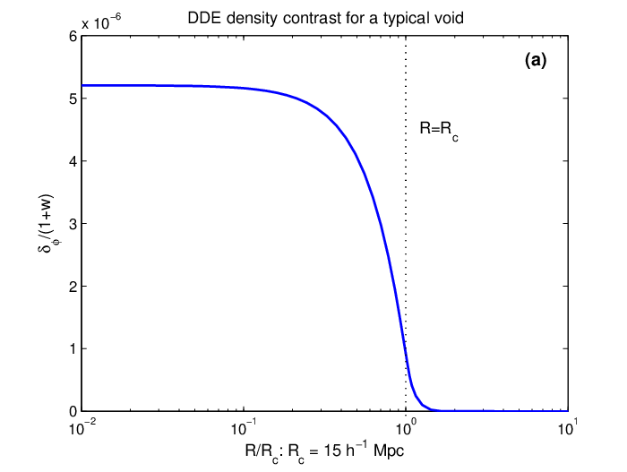

Recently, there has been a great deal of discussion, both theoretical and observational, about the possibility that extremely large voids () exist within the visible Universe (Rudnick, Brown & Williams 2007; Inoue & Silk 2006). Additionally, a number of authors have speculated that we may even be living inside such an object (Schwarz & Weinhorst 2007; Conley et al. 2007; Zehavi et al. 1998; Giovanelli et al. 1999). For example, Rudnick, Brown & Williams 2007 showed that both the WMAP cold spot and an observed dip in the surface brightness and number counts of extragalactic radio sources could be explained by the presence of an almost completely empty at . Inoue & Silk 2006 showed that the ISW effect due to a void with and would be observed as cold spots with a temperature anisotropy , which might explain the observed large-angle CMB anomalies. If extremely large voids such as these exist they would be associated with the largest DDE overdensities within the visible Universe. In Figure 14 we plot the profile for both the , object postulated by Rudnick, Brown & Williams 2007 and for the , void considered by Inoue & Silk 2006. In the former case we find and in the latter . These values of are about two orders of magnitude larger than those associated with a typical void. However, even around such extremely large voids we still find that the DDE perturbation is small: .


VI.4. ISW Effect due to DDE clustering
We have seen that the DDE density contrast, , is always small with magnitude for average sized structures in the Universe. The Integrated Sachs Wolfe (ISW) effect is highly sensitive to the presence of dark energy. In a purely matter dominated universe, the ISW effect vanishes entirely for linear perturbations. We shall see that the DDE contribution to the ISW from a cluster with radius is proportional to and so we consider only large (but still sub-horizon) scales. On such scales the matter perturbation is small and we are in the linear regime. The ISW effect is most easily derived in the conformal Newtonian gauge in which the metric takes the form:
Since we are dealing with shearless matter, to leading order, and, in momentum space:
| (35) | |||||
where and and are defined in the rest frame of the matter particles. Using Eq. (19) we see that:
| (36) | |||||
The temperature anisotropy due to the ISW effect is given by:
where is the value of today and is its value on the surface of last scattering and . The contribution to from the matter perturbation is:
and at late times, whereas the contribution to from the DDE clustering is:
where and
It follows that:
assuming that or smaller in the recent past then:
We found above that the largest DDE perturbations would mostly likely be associated with large voids of matter, with for a void with central matter density contrast (Inoue & Silk 2006, such as that considered by). In this case we would have:
which is at most . In the absence of DDE clustering, the ISW temperature anisotropy of such a void was found to be . We therefore predict that the DDE clustering contribution to the temperature anisotropy would be at most . For smaller objects (with radius ) the DDE ISW temperature anisotropy scales as .
In conclusion: the ISW due to sub-horizon DDE clustering in models where the dark energy is due to a minimally coupled scalar field with canonical kinetic term is always suppressed by a factor of about relative to the ISW effect to the matter perturbation itself. It therefore seems unlikely that the DDE contribution detected against the background of the ISW effect caused by the matter.
VI.5. Discussion
In this section we have applied our results to evaluate the profile and evolution of in the vicinity of typical galaxy clusters, superclusters and voids. We found that, today, the largest inhomogeneities in the DDE energy density value should occur in the vicinity of supervoids such as the one in Boötes (Kirschner et al. 1981). At the centre of a supervoid we predict . At the centre of a galaxy cluster, supercluster or average sized void, we found ; with for both virialised clusters and voids, and for superclusters. Generally for supervoids, and for other structures. Recently there has been a fair amount of interest in the possibility that extremely large voids might exists with radii . Even for objects as large as this, however, we found that .
Given the current bounds on the dark energy (EoS) parameter: , our results imply that if dark energy is described by a canonical scalar field that does not couple to (or only couples very weakly to) matter and is minimally coupled to gravity, then its energy density today is virtually homogeneous with largest fluctuations no larger than 1 part in (or possibly one part in if voids exist). Indeed, typical fluctuations in the DDE energy density will be smaller than a few parts in . We found that superclusters are generally associated with small, local DDE voids whereas most other structures (galaxies and voids of matter) are associated with local overdensities of dark energy.
VII. Summary and Conclusions
In this paper we have studied how dynamical dark energy clusters over sub-horizon scales in theories where the dark energy is described by a canonical scalar field with no coupling to matter. Sub-horizon dark energy clustering in such models has always been expected to be small, but previous studies of it have assumed the matter perturbation to be small and have, for the most part relied on numerical simulations. In this paper, however, we used the powerful method of matched asymptotic expansions to derive an analytic expression, Eq. (18), for the DDE density contrast in terms of the peculiar velocity and density contrast of the matter. Our equation for holds not only in the linear regime, where the matter density contrast is small, , but also in the far more interesting but far less studied quasi-linear and non-linear regimes where or greater.
There were then essentially two parts to this paper, finding an expression for as a function of , and , and then evaluating this. The evaluating part is only done approximately for models that look sufficiently like . So that to a first approximation we can use to get , and . Different dark energy models would give different predictions but just from the form of one can see that unless very large deviations from the predictions of , and occur then will be well approximated by taking a background.
Our key assumption in deriving our formula for was that the matter density contrast is only or greater on scales that are small compared to the Hubble length, . This assumption holds very well for typical structures such as galaxies, clusters, superclusters and voids. We also made a number of simplifying assumptions:
- •
We assumed spherical symmetry. Although our interest is in dark energy rather than varying-constants, the sub-horizon dynamics of perturbations in the DDE scalar field are very similar to those of the scalar fields in varying-constant models provided one sets the matter coupling in such theories to zero. (Shaw & Barrow 2006a; Shaw & Barrow 2006b; Shaw & Barrow 2006c) studied the evolution of a light scalar field in an inhomogeneous background in the context of varying-constant. Both spherically symmetric backgrounds and ones without any symmetries were considered, and it was found that deviations from spherically symmetry did not alter the leading order behaviour of the scalar field perturbations when the matter coupling vanishes. Therefore, whilst the assumption of spherical symmetry can be relaxed, we do not expect it to greatly alter our results.
- •
We assumed that we were not near a black hole horizon. This assumption allowed us to take on sub-horizon scales. This assumption could also be relaxed, and once again both the form of and its magnitude are not expected to be greatly effected. We again base this expectation on the results found for light scalars in the context of varying-constants by Barrow & Shaw 2007.
- •
We assumed that the mass of the scalar field, , was very small compared to , where in the length scale of the peak in the matter density contrast. This assumption could be done away with, however it would significantly complicate the analysis in the non-linear regime. Moreover since we have require and in most quintessence models , it is for most models generally true that . If or larger, then we expect that it will result in a smaller DDE density contrast, i.e. smaller values of .
One of the main motivations for this work was the recent work of Dutta & Maor 2007. They studied the clustering of a subclass of the DDE models which we have looked at in this work. They numerically evolved the linearized field equations for both and the metric. In the regime where the linearized equations are valid (i.e. ), our analytical results agree with theirs: shortly after the collapse begins, is positive, but then as the dying mode of an overdensity of matter becomes small, changes sign and becomes negative. At late times in the linear regime an overdensity of matter corresponds to a DDE void, and vice versa. We saw in this paper that this correspondence continues to hold in the quasi-linear regime, , that is appropriate for superclusters and voids of matter. When , Dutta and Maor found that could grow to be relatively large (of the order of ), and that this could lead to corrections to the equation of state parameter, , of the order of a few percent. However, as we noted in the introduction, the values of for which this effect was found fall outside the regime where the linearized field equations which they used are actually valid. One should point out however, that in a matter dominated universe (), there is a clear mapping between the the linear regime of an overdensity and the exact fully developed non- linear overdensity. Presumably, such mapping should occur also in the presence of a scalar field, though the multiple change of sign of the DDE perturbation complicate things considerably and this relation is not straight forward. We also saw that at late times in the linear and quasi-linear regimes grows faster than . If it were not for the onset of truly non-linear behaviour in the evolution of , this would indeed lead to large values of seen at late times by Dutta & Maor 2007.
In our study we found that for realistic astrophysical objects is very small, indeed it is generally . The fast growth in seen by Dutta & Maor 2007 for should therefore been interpreted as resulting from applying linearized field equations outside their realm of validity, rather than a true physical effect. Furthermore, at very late times when the matter perturbation has virialised and accretion onto the core has all but ceased, we found that , and that , where is the smallest radius for which decreases as quickly as , is the mass inside .
Whilst it is possible with highly non-linear potentials, in general it seems improbably that values of , which in turn result in order values for will result in any pronounced non-linear effects especially over sub horizon scales. It is fair to say though that the conditions might be on the brink of breaking down for a Mpc void, since . But for smaller objects provided the conditions we place on the potential hold (which essentially preclude small changes in from resulting in huge changes in , or ) then there is no particular reason to think that perturbations in will result in or greater corrections to . One should also point out that in the case where the scalar field is strongly coupled to matter ( e.g. as in (Mota & Shaw 2006; Brax et al. 2004; Mota & Shaw 2006)), then the dark energy perturbations might not be small. Since it is natural to expect that when matter starts to infall into the nonlinear regime it will drag along the dark energy field.
We also used our analytical expression for to calculate the Integrated Sachs Wolfe (ISW) induced by the DDE density perturbations. We found that the ISW due to the DDE perturbations is always much smaller than the ISW effect due to the matter perturbation in these DDE models by a factor of roughly . Indeed, even the ISW effect due to the clustering of DDE near an extremely large is found to result in a temperature anisotropy no larger than . For smaller objects the ISW effect due to DDE clustering scales as (where is the radius of the cluster). It is therefore unlikely that, if dark energy is described by a simple uncoupled quintessence theory, DDE perturbations will be detected through the ISW effect.
In summary: we have derived an analytical expression for the DDE density contrast in uncoupled quintessence models and used it to make quantitative predictions for DDE clustering. Our results should also apply to fields with very weak matter coupling. This analysis could also be straightforwardly extended to models that are coupled to matter but we leave this to a later work. If the mass of the scalar in these models is , then is, to leading order, independent of the specifics of the underlying theory. As opposed to what has been suggested elsewhere, we found that is always small compared to the matter density contrast, and that even when the matter perturbation goes non-linear, remains for typical astrophysical objects. If we define the radius, , of a matter over/under - density by the condition that at , the mean matter density contrast drops off like , then we found that . DDE clustering could potentially be detected through the ISW effect or measurements of the peculiar velocity field of matter. Roughly, the magnitude of the DDE clustering contribution to these effects is a factor times the contribution from the clustering of ordinary matter. For realistic astrophysical objects, we found that voids and super-voids correspond to local overdensities in dark energy, with for clusters and average voids, and for super-voids. If voids with radii of exist within the visible Universe then may be as large as . Linear overdensities of matter and super-clusters generally correspond to local voids in dark energy; for a typical super-cluster: .
Astronomical observations indicate for , and so we conclude that if dark energy is described by an uncoupled quintessence model, then today dark energy is almost homogeneous on sub-horizon scales with perturbations generally of order of ; the largest perturbations will be and associated with very large voids of matter.
Acknowledgements
We thank S. Dutta and I. Maor for the many useful comments and suggestions on this work. DFM is supported by the Alexander von Humboldt Foundation. DJS is supported by PPARC
References
- Abramo et al. (2007) Abramo L. R., Batista R. C., Liberato L. and Rosenfeld R. (2007), arXiv:0707.2882 [astro-ph].
- Adelman-McCarthy et al. (2006) Adelman-McCarthy J. K. et al. (2006), Astrophys. J. Suppl. 162 38.
- Amendola (2000) Amendola L. (2000), Phys. Rev. D 62, 043511.
- Amarzguioui et al. (2006) Amarzguioui M., Elgaroy O., Mota D. F. and Multamaki T. (2006), Astron. Astrophys. 454 707.
- Balaguera-Antolínez, Mota & Nowakowski (2006) Balaguera-Antolínez A., Mota D. F. and Nowakowski M. (2006), Class. Quant. Grav 23, 4497-4510.
- Balaguera-Antolínez, Mota & Nowakowski (2007) Balaguera-Antolínez A., Mota D. F. and Nowakowski M. (2007), to appear in Mon. Not. Roy. Astro. Soc..
- Bardelli et al. (2000) Bardelli S., Zucca E., Zamorani G., Moscardini L. and Scaramella R. (2000), Mon. Not. Roy. Astro. Soc. 312, 540.
- Barrow & Shaw (2007) Barrow J. D. and Shaw D. J. (2007), Gen. Rel. Grav. to appear in Obregon’s Festschrift.
- Bartelmann, Doran & Wetterich (2005) Bartelmann M., Doran M. and Wetterich C. (2005), [arXiv:astro-ph/0507257].
- Bondi (1947) Bondi H., Mon. Not. R. astron. Soc. 107, 410 (1947)
- Bolejko, Krasiński & Hellaby (2005) Bolejko K., Krasiński A. and Hellaby C. (2005), Mon. Not. Roy. Astron. Soc. 362, 213.
- Brax et al. (2004) Brax et al. 2004 Phys.Rev.D70, 123518.
- Brookfield et al. (2006a) Brookfield A. W. et al. (2006), Phys. Rev. Lett. 96, 061301.
- Brookfield et al. (2006b) Brookfield A. W., van de Bruck C., Mota D. F. and Tocchini-Valentini D. (2006b), Phys. Rev. D 73, 083515.
- Caimmi (2007) Caimmi R., 2007, New Astron.12:327-345.
- Capozziello, Cardone & Troisi (2005) Capozziello S., Cardone V. F. and Troisi A. (2005), Phys. Rev. D 71, 043503.
- Conley et al. (2007) Conley A. et al. (2007), arXiv:0705.0367 [astro-ph];
- Corasaniti, Giannantonio & Melchiorri (2005) Corasaniti P., Giannantonio T and Melchiorri A. (2005), Phys. Rev. D 71, 123521.
- Dey, Strauss & Huchra (1990) Dey A., Strauss M. A. and Huchra J. (1990), Astron. J. 99, 463.
- Doran, Robbers & Wetterich (2007) Doran M., Robbers G. and Wetterich C. (2007), Phys. Rev. D 75, 023003.
- Dutta & Maor (2007) Dutta S. and Maor I. 2007, Phys. Rev. D 75, 063507.
- Dvali, Gabadadze & Porrati (2000) Dvali G. R., Gabadadze G. and Porrati M. (2000), Phys. Lett. B 485, 208.
- Geller, Diaferio & Kurtz (1999) Geller M. J., Diaferio A. and Kurtz M. J. (1999), Astrophys. J. 517, L23.
- Giovanelli et al. (1999) Giovanelli R. et al. (1991), Astrophys. J. 525 25.
- Hamilton et al. (1991) Hamilton A. J. S., Kumar P., Lu E., Mathews A. (1991), Astrophys J., 374, L1.
- Hannestad & Mortsell (2002) Hannestad S. and Mortsell E. (2002), Phys. Rev. D 66, 063508.
- Hinch (1991) Hinch E. J. (1991), Perturbation methods, (CUP, Cambridge).
- Hoyle & Vogeley (2004) Hoyle F. and Vogeley M. S. (2004), Astrophys. J. 607, 751.
- Hoffman (1986) Hoffman Y. (1986), Astrophys. J. 308, 493.
- Inoue & Silk (2006) Inoue K. T. and Silk J. (2006), [arXiv:astro-ph/0612347]
- Kirschner et al. (1981) Kirschner R. P., Oemler A., Schechter P. L. and Shectman S. A. (1981), Astrophys. J. 248, L57.
- Kirschner et al. (1987) Kirschner R. P., Oemler A., Schechter P. L. and Shectman S. A. (1987), Astrophys. J. 314, 493.
- Koivisto & Mota (2006) Koivisto T. and Mota D. F. (2006), Phys. Rev. D 73, 083502 [arXiv:astro-ph/0512135].
- Koivisto & Mota (2007a) Koivisto T. and Mota D. F. (2007a), Phys. Lett. B 644, 104 (2007).
- Koivisto & Mota (2007b) Koivisto T. and Mota D. F. (2007b), Phys. Rev. D 75, 023518 (2007).
- Kolb Matarrese & Riotto (2006) Kolb E., Matarrese S. and Riotto A. (2006), New J.Phys. 8 322.
- Lahav et al. (1991) Lahav O. et al. (1991), Mon. Not. Roy. Astro. Soc. 251 128.
- Linder & White (2005) Linder E. and White M. (2005), Phys. Rev. D 72, 061304.
- Mainini (2005) Mainini R. (2005), Phys. Rev. D 72, 083514.
- Manera & Mota (2006) Manera M. and Mota D. F. (2006), Mon. Not. Roy. Astron. Soc. 371 1373 [arXiv:astro-ph/0504519].
- Moffat (2006) Moffat J. W. (2006), J. Cosmol. Astropart. Phys. 05.
- Maor & Lahav (2005) Maor I. and Lahav O. (2005), [arXiv:astro-ph/0505308].
- Mota & van de Bruck (2004) Mota D. F. and van de Bruck C.(2004), Astron. Astrophys. 421, 71.
- Mota & Shaw (2006) Mota D. F., Shaw D. J., 2006, Phys.Rev.Lett. 97, 151102
- Mota & Shaw (2006) Mota D. F., Shaw D. J. ,2007, Phys. Rev. D 75, 063501
- Navarro, Frenk & White (1997) Navarro J. F., Frenk C. S. and White S. D. M. (1997), Astrophys. J. 490, 493.
- Nojiri & Odintsov (2003) Nojiri S. and Odintsov S. D. (2003), Phys. Rev. D 68, 123512.
- Nunes & Mota (2006) Nunes N. J. and Mota D. F. (2006), Mon. Not. Roy. Astron. Soc. 368:2 751 [arXiv: astro-ph/0409481].
- Nunes, da Silva & Aghanim (2005) Nunes N. J., da Silva A. C. and Aghanim N. (2005), [arXiv:astro-ph/0506043].
- Peebles & Ratra (1988) Peebles P. J. E. and Ratra B. (1998), ApJ 325, L17.
- Peebles (1980) Peebles P. J. E. (1980), The large scale structure of the Universe, Princeton University Press.
- Pettorino, Baccigalupi & Mangano (2005) Pettorino V., Baccigalupi C. and Mangano G. (2005), JCAP 0501, 014.
- Percival (2005) Percival W. J. (2005), [arXiv:astro-ph/0508156].
- Perlmutter et al. (1999) Perlmutter S. et al. (1999), Astrophys. J. 517, 565.
- Riess et al. (1998) Riess A. G. et al. (1998), Astron. J. 116, 1009.
- Riess et al. (2004) Riess A. G. et al. (2004), Astron. J. 607, 665.
- Riess et al. (2006a) Riess A. G. et al. (2006a), to appear in Astrophys. J.
- Riess et al. (2006b) Riess A. G. et al. (2006b), [arXiv:astro-ph/0611572].
- Rudnick, Brown & Williams (2007) Rudnick L., Brown, S. and Williams L. R. (2007), arXiv:0704.0908 [astro-ph]
- Schwarz & Weinhorst (2007) Schwarz D. J., Weinhorst B. (2007), arXiv:0706.0165 [astro-ph];
- Shaw & Barrow (2006a) Shaw D. J. and Barrow J. D. (2006a), Phys. Rev. D 73, 123505.
- Shaw & Barrow (2006b) Shaw D. J. and Barrow J. D. (2006b), Phys. Rev. D 73, 123506.
- Shaw & Barrow (2006c) Shaw D. J. and Barrow J. D. (2006c), Phys. Lett. B 639, 596.
- Shaw & Mota (2007) Shaw D. J. and Mota D. F. (2007), to appear in Astrophys. J. Supp.
- Spergel et al. (2003) Spergel D. et al. (2003), Astrophys. J. Suppl. 148, 175.
- Spergel et al. (2007) Spergel D. et al. (2007), Astrophys. J. Suppl. 170, 377.
- Tegmark et al. (2006) Tegmark M. et al. (2006), Phys. Rev. D 74 123507.
- Tolman (1934) Tolman R. C. (1934), Proc. Nat. Acad. Sci. USA 20, 169.
- Tully (1982) Tully R. B. (1982), Astrophys. J. 257, 389.
- Wang (2006) Wang P. (2006), Astrophys. J. 640, 18.
- Wang & Steinhardt (1998) Wang L. and Steinhardt P. (1998), Astrophys. J. 508, 483.
- Weller & Lewis (2003) Weller J. and Lewis A. M. (2003), Mon. Not. Roy. Astron. Soc. 346, 987.
- Wetterich (1988) Wetterich C. (1988), Nucl. Phys. B302, 668.
- Wood-Vasey et al. (2007) Wood-Vasey W. M. et al. (2007), astro-ph/0701041.
- Zehavi et al. (1998) Zehavi I. et al. (1998), Astrophys. J. 503 483.