Bright branes for strongly coupled plasmas
Abstract:
We use holographic techniques to study photon production in a class of finite temperature, strongly coupled, large- quark-gluon plasmas with quark flavours. Our results are valid to leading order in the electromagnetic coupling constant but non-perturbatively in the interactions. The spectral function of electromagnetic currents and other related observables exhibit an interesting structure as a function of the photon frequency and the quark mass. We discuss possible implications for heavy ion collision experiments.
Keywords:
D-branes, Supersymmetry and Duality, Brane Dynamics in Gauge Theories1 Introduction
Photons emitted by the quark-gluon plasma (QGP) created at the Relativistic Heavy Ion Collider (RHIC), as well as in future heavy ion experiments at the Large Hadron Collider (LHC), are expected to be an important probe of the plasma physics. Because of the finite extent of the plasma ball and of the weakness of the electromagnetic coupling constant, once a photon is produced it escapes essentially undisturbed, thus carrying valuable information about local properties of the plasma at the point of emission [1].
At weak coupling, photon production in Quantum Chromodynamics (QCD) can be studied by means of perturbation theory [2]. However, results from RHIC seemingly indicate that the plasma created there does not behave as an almost free gas of quarks and gluons, but rather as a strongly coupled liquid [4]. Consequently, understanding the spectrum and rate of photon emission requires a non-perturbative calculation. This is currently beyond the scope of analytical methods, and performing this calculation on the lattice is problematic due to the real-time, Lorentzian-signature nature of the physics involved.
In view of the above, it is interesting to investigate photon production in the context of the gauge/gravity correspondence [5]. Although the gravity dual of QCD itself is not known, the duals of a large class of finite-temperature, strongly coupled, large- gauge theories are known. One may hope that generic, universal features exhibited by such theories may be useful indications as to the behaviour of QCD, at least in the regime of strong coupling. With this in mind, ref. [6] studied photon production at strong coupling in super Yang-Mills (SYM), a four-dimensional theory with massless matter in the adjoint representation, and ref. [7] calculated the rate of photon emission in a four-dimensional theory with massless quarks. One purpose of this paper is to study the effect of a non-zero quark mass on photon production.
In perturbative, weak-coupling calculations it is usually assumed that the temperature is high enough so that the thermal quark mass, of order (with the ’t Hooft coupling) is much larger than the bare, zero-temperature quark mass , and so the latter is effectively set to zero. Regardless of the precise temperature range in which this is applicable, the very nature of this approximation assumes that quarks are well defined quasi-particles to which physical properties such as a thermal mass can be meaningfully assigned. This is true at sufficiently weak values of the coupling, but it is not necessarily true at strong coupling. Well defined quasi-particle excitations certainly do not seem to exist in the phases of interest of the holographic theories that we will consider [8, 9], and they might not exist either in a QCD plasma at temperatures just above deconfinement. Under these circumstances, the bare quark mass is better thought of as a microscopic parameter on which the physics depends, but without a direct interpretation as the mass of a physical quasi-particle. Examples of physical quantities that depend on the quark mass through the dimensionless combination include the entropy density [8, 9], the shear viscosity [10], etc. We will see that the same is true for observables related to photon production.
We will consider finite-temperature, super Yang-Mills (SYM) theories coupled to flavours of fundamental matter whose bare mass is an adjustable parameter. The fundamental matter includes both fermions and scalars, which we will refer to collectively as ‘quarks’. Our goal is to study photon production as a function of the quark mass and the photon frequency, to leading order in the electromagnetic coupling constant but non-perturbatively in the interactions. Note that, in addition to the quarks, the matter content in these theories also includes adjoint fields. Since we would like to model as closely as possible QCD, which has no adjoint matter, we will assume that the photon couples directly only to the quarks, i.e., we will assign vanishing electric charge to the adjoint matter.
In the limit of a small number of flavours, , the theories above possess a simple dual description in terms of Dq-brane probes in the gravitational background of Dp-branes [11]. At temperatures high enough so that the gluons (and the adjoint matter) are deconfined, the gravitational background contains a black hole [12], represented by the shaded blob in fig. 1. In this deconfined phase, the fundamental matter may still be in two different phases separated by a first-order phase transition [9].11 1 Specific examples of this transition were originally seen in [13, 14]. Aspects of these transitions were independently studied in the D3/D7 system in [15, 16], and in a slightly different framework in [17].

From the viewpoint of the holographic description, the basic physics behind this transition is easily understood. The asymptotic distance between the Dq-branes and the black hole is proportional to the quark mass, whereas the size of the black hole horizon is proportional to the temperature. Thus, for sufficiently small , the Dq-branes are deformed by the gravitational attraction of the black hole, but remain entirely outside the horizon in what we call a ‘Minkowski embedding’ (see fig. 1). However, above a critical temperature , the gravitational force overcomes the tension of the branes and these are pulled into the horzion. We refer to such configurations as ‘black hole embeddings’. In between these two types of embeddings there exists a ‘critical embedding’ in which the branes just ‘touch the horizon at a point’. However, thermodynamic considerations reveal that a first-order phase transition occurs between a Minkowski and a black hole embedding. In other words, the critical embedding is skipped over by the phase transition, and near-critical embeddings turn out to be metastable or unstable.
In the dual field theory, this phase transition is exemplified by discontinuities in physical quantities such as, for example, the quark condensate or the contribution of the fundamental matter to the entropy density. However, the most striking feature of this phase transition is found in the spectrum of physical excitations of the fundamental matter. In the low-temperature, Minkowski phase the spectrum is gapped and contains a discrete set of deeply bound mesons (i.e., quark-antiquark bound states) with masses of order . These mesons are dual to excitations supported on the probe branes – see, e.g., [18, 19, 20]. In addition, the Minkowski-phase spectrum also contains well defined, quark-like excitations described by strings stretching between the tip of the branes and the horizon. These have masses of order and are therefore parametrically heavier than the mesons. Both sets of excitations are absolutely stable in the large-, strong coupling limit under consideration.
In the high-temperature, black hole phase stable mesons cease to exist. Rather one finds a continuous and gapless spectrum of excitations [8, 9, 21, 22]. Hence the mesons dissociate or ‘melt’ at the first order phase transition at , and beyond it no well defined, quasi-particle notion of an individual quark exists, since a string stretching between any point on the branes and the horizon will quickly fall through the horizon. In the gauge theory this corresponds to the fact that any localised quark charge will quickly spread across the entire plasma, thus loosing its identity.
In this paper we will study photon production in the black hole phase. We will see that this is proportional to , i.e., to the number of electrically charged degrees of freedom, as one would expect. For our result coincides with that of [6], except for the fact that in that reference the overall normalisation is set by , reflecting the fact that electric charge is carried by adjoint degrees of freedom. We stress that the photon production we will calculate is not a correction to an -result but the leading result in the large- expansion, since in our case the adjoint matter is electrically neutral. We will see that the gravity picture provides a simple, geometric explanation for the agreement (up to normalisation) between our result and that of [6].
We will not explicitly study photon production in the Minkowski phase, since we have a clear expectation of what the result would be. Indeed, as explained above, in this phase the spectrum consists of a discrete set of stable modes, so we expect the spectral function (4) to be given by a sum of delta functions supported at appropriate values of the momentum. We will confirm this expectation indirectly by calculating the spectral function for black hole embeddings near the critical embedding (see fig. 1).
In order to study photon production, one must in principle introduce a dynamical photon that couples appropriately to the fundamental matter and construct the dual of the gauge theory thus obtained. However, we will see that, to leading order in the electromagnetic coupling constant, photon production in the theory is completely determined by correlators in the original theory with no dynamical photon. This observation allows the holographic calculation of the desired correlators.
This paper is organised as follows. In sec. 2 we discuss how to calculate the rate of photon production in a gauge theory at finite temperature. In sec. 3 we explain how to use the holographic description in terms of a Dp/Dq system to study photon production in the dual gauge theory. In secs. 4 and 5 we present our results for the D3/D7 and the D4/D6 systems, respectively. We conclude in sec. 6 with a discussion of our results and their possible implications for heavy ion collision experiments.
2 Photon emission in a hot gauge theory
Consider a -dimensional gauge theory with flavours of fundamental fermions and scalars , , to which we will collectively refer as ‘quarks’. Imagine coupling this theory to electromagnetism by introducing and additional, dynamical, Abelian gauge field, the photon, that couples to the fundamental fields with strength (electric charge) .22 2 For simplicity we assume that all the fundamental fields have equal mass and carry equal electric charge, but our results can be generalised straightforwardly. Later we will consider theories that also contain adjoint matter. Since our goal is to model QCD, which has no such matter, we will assign vanishing electric charge to the adjoint fields. This new theory may be constructed by adding a kinetic term for the photon and replacing the -covariant derivative by when acting on the fundamental fields, with . In this way we obtain an gauge theory with Lagrangean
| (1) |
where and the electromagnetic current is given by
| (2) |
A sum over flavour and colour indices is implicit in this formula. Note that the photon field enters this current through the covariant derivative acting on the scalars.
In thermal equilibrium, the differential photon emission rate per unit time and volume, at leading order in the electromagnetic coupling constant , is then given by [23]
| (3) |
where is the photon null momentum,
| (4) |
is the spectral density, and
| (5) |
is the retarded correlator of two electromagnetic currents, whose diagramatic representation (including photon fields as external legs) is given in fig. 2.
 |
 |
| (a) | (b) |
Finally,
| (6) |
is the standard Bose-Einstein distribution function. Without loss of generality we will assume that points in the -direction, and we will denote by , the remaining spatial directions. The polarisation vectors may be chosen to be unit spatial vectors orthogonal to . Transversality of the correlator implies that the sum over polarisation vectors in (3) may be replaced by the trace of the spectral function, i.e.,
| (7) |
and rotational invariance ensures that this is given by
| (8) |
where
| (9) |
The trace of the spectral function also determines the electric conductivity as
| (10) |
Thus in order to study photon production we must in principle calculate the two-point function (5) in the theory. However, as noted in [6], to leading order in the electromagnetic coupling constant this reduces to a calculation purely within the original theory; this is the key observation that will allow us to perform this calculation using the dual gravitational description, since the dual of the theory is unknown. To see this, note first that the terms in the electromagnetic current (2) proportional to the photon field (implicit in the covariant derivative) lead to higher-order contributions in to the correlator (5), and can thus be ignored to leading order in . Second, observe that the two-point function of the remaining terms in the current can be calculated in the theory, since again the effects of including the dynamical photon are of higher order in . Diagramatically, this means that no photon fields are present in the shaded blobs in fig. 2. An additional observation is the fact that the tadpole diagram in fig. 2 has no imaginary part and hence does not contribute to the desired spectral function.
We therefore conclude that, to leading order in the electromagnetic coupling constant, photon production in an theory is completely determined by the two-point function of the electromagnetic current in the theory. In the rest of the paper we will calculate this correlator in SYM theories coupled to fundamental matter.
3 Holographic description
In the decoupling limit, the black Dp-brane solution in the string frame takes the form
| (11) |
where ,
| (12) |
and is a length scale (the AdS radius in the case ). The horizon lies at . As usual, regularity of the Euclidean section, obtained through , requires that be identified with period
| (13) |
In this paper it will be useful to work with a different radial coordinate related to through
| (14) |
in terms of which and the horizon lies at .
According to the gauge/gravity correspondence, string theory on the background above is dual to -dimensional, maximally supersymmetric Yang-Mills theory at temperature . In some cases one periodically identifies some of the ‘Poincare’ directions in order to render the theory effectively lower-dimensional at low energies; a prototypical example is that of a D4-brane with one compact space direction. Under these circumstances a different background with no black hole may describe the low-temperature physics, and a phase transition may occur as increases [12]. In the gauge theory this is typically a confinement/deconfinement phase transition for the gluonic (and adjoint) degrees of freedom. Throughout this paper we assume that is high enough, in which case the gauge theory is in the deconfined phase and the appropriate gravitational background is (3).
Consider now coincident Dq-brane probes that share spacelike Poincaré directions with the background Dp-branes and wrap an inside the . We will assume that the Dq-branes also extend along the radial direction, so that . We will denote by , with , the directions common to both branes. In the gauge theory the Dq-branes correspond to introducing flavours of fundamental matter of equal mass that propagate along a -dimensional defect. To ensure stability, we will assume that the Dp/Dq intersection under consideration is supersymmetric at zero temperature. Under these conditions the Ramond-Ramond field sourced by the Dp-branes does not couple to the Dq-branes. Two cases of special interest here are the D3/D7 () [13] and the D4/D6 () [14] systems. If one of the D4 directions is compact, then both cases can effectively be thought of as describing the dynamics of a four-dimensional gauge theory with fundamental matter.
The gauge symmetry on the Dq-branes is a global, flavour symmetry of the gauge theory. If this theory is coupled to electromagnetism as explained in the previous section (in particular, if all flavours are assigned equal electric charge ), then the electromagnetic current is the conserved current associated to the overall . In order to study photon emission to leading order in it suffices to evaluate the correlator (5) in the gauge theory with no dynamical photon.
At strong ’t Hooft coupling and large , this correlator is easily calculated holographically. Indeed, global symmetries of the gauge theory are in one-to-one correspondence with gauge symmetries on the gravity side, and each conserved current of the gauge theory is dual to a gauge field on the gravity side [24]. Let , , be the guage field associated to the overall gauge symmetry on the Dq-branes. Upon dimensional reduction on the -sphere wrapped by the Dq-branes, gives rise to a massless gauge field , massless scalars, and a tower of massive Kaluza-Klein (KK) modes. All these fields propagate on the non-compact dimensions of the Dq-branes. We will work in the gauge , and we will consistently set to zero the scalars and the higher KK modes, since they are not of interest here. The gauge field is the desired dual to the conserved electromagnetic current of the gauge theory; just like the quarks are localised on a defect inside the gauge theory, the dual gauge field is localised on the Dq-branes inside the bulk spacetime.
According to the gauge/gravity correspondence, correlation functions of can be calculated by varying the string partition function with respect to the value of at the boundary of the spacetime (3). Under the present circumstances, the string partition function reduces to , where is the sum of the supergravity action and the effective action for the Dq-branes. Since does not enter the supergravity action, the form of this action will not be needed here. Moreover, the Wess-Zumino part of the Dq-branes action does not contribute for the brane orientations and the gauge field polarisations considered in this paper. Therefore, it suffices to consider the Dirac-Born-Infeld part of the Dq-branes action:
| (15) |
where is the induced metric on the Dq-branes, is the overall field strength, is the Dq-brane tension, and and are the string length and coupling constant, respectively. Since we are only interested in the two-point function (5), we only need to keep terms up to quadratic order in the gauge field. We will therefore work with the simpler action
| (16) |
where .
The Dq-branes wrap an -sphere in the directions transverse to the Dp-branes, so it is convenient to write the metric on in adapted coordinates as
| (17) |
Setting , the Dq-branes embedding may then be specified as . Asymptotically, i.e., as or , this behaves as [8, 9]
| (18) |
where and are proportional to the quark mass and condensate, respectively (see below).
Since the gauge field enters the action (16) quadratically, turning on induces a correction of order on the branes embedding. When the action is evaluated on-shell, this generates a boundary-term contribution of the form
| (19) |
where is the Dq-branes Lagrangean density and . Since , this has in principle the right form to contribute to the two-point function (5). However, as explained in [9], this contribution is proportional to , and hence vanishes because the quark mass must be kept fixed in computing the correlator.
We thus conclude that, in order to calculate the photon emission rate, we may consistently proceed by first determining the Dq-branes embedding in the absence of the gauge field, and then solving for the gauge field on that embedding. As explained above, we will set to zero the components of the gauge field on the -sphere wrapped by the Dq-branes. Moreover, following [25], we will choose the gauge , Fourier-decompose the remaining components of the gauge field as
| (20) |
and choose to point in the -direction. Under these circumstances the equations of motion for the -components of the gauge field that follow from the action (16) decouple from each other and from those for . Setting , the equation of motion takes the form
| (21) |
where we have made use of the fact that . The functions depend on the embedding and will be specified below. Eq. (21) may be consistently derived from the ‘reduced’ action
| (22) |
obtained from (16) by integrating over the -sphere and setting . We will see below that the normalisation constant in front of this action scales as and determines the overall magnitude of photon production.
According to the prescription in [26, 27], the retarded correlator (9) is then given by
| (23) |
where and is a solution of the equation of motion (21) obeying the incoming-wave boundary condition at the horizon. The imaginary part of , which is all we need, is -independent, and it is convenient to calculate it at the horizon instead of at the boundary:
| (24) |
Note that, although not explicitly indicated, several quantities above depend not only on the photon frequency but also on the quark mass, since the equation of motion (21) that determines depends on the branes embedding through the functions and .
4 The D3/D7 system
Here we will specialise the above discussion to the D3/D7 system. This intersection is summarised by the array
| (25) |
Of course, this is an interesting system because , i.e., both the gluons and the fundamental fields in the gauge theory propagate in dimensions.
The metric (3) for black D3-branes takes the form
| (26) |
where
| (27) |
In this case the dimensionless coordinate (14) is33 3 This is related to the coordinate used in [25] as . , in terms of which the metric becomes
| (28) |
Specifying the D7-branes embedding through , as explained above, the induced metric takes the form
| (29) |
In this case the asymptotic behaviour of is44 4 In this limit, the coordinate used here and the coordinate used in [8, 9] are related through .
| (30) |
where the dimensionless constants and are related to the quark mass and condensate, respectively, through [8, 9]:
| (31) | |||||
| (32) |
with the ’t Hooft coupling. The operator is a supersymmetric version of the quark bilinear, and it takes the schematic form
| (33) |
where is one of the adjoint scalars. We will loosely refer to its expectation value as the ‘quark condensate’. A detailed discussion of this operator, including a precise definition, can be found in the appendix of ref. [28].
Eq. (31) implies the relation between the dimensionless quantity , the temperature and the mass scale
| (34) |
where is the mass of the lightest meson (i.e., the mass gap) in the discrete meson spectrum at zero temperature [18, 19, 20, 14]. determines the scale of the temperature of the phase transition for the fundamental degrees of freedom, , since the latter takes place at .
The functions occurring in the reduced action (22) are given in this case by
| (35) |
and the normalisation constant is
| (36) |
where
| (37) |
is the normalisation constant introduced in [8, 9] and is the volume of a unit three-sphere.
Analysis of eq. (21) near reveals that the solution obeying the incoming-wave boundary condition behaves as near the horizon. We will thus seek a solution of the form
| (38) |
where is a regular function of and the second factor has been explicitly extracted for convenience. Since the differential equation solved by is linear, its overall normalisation is arbitrary, and it cancels out in eqs. (23), (24). We choose to fix it by setting equal to unity at the horizon, i.e., . Using the form of the solution (38) and this normalisation choice for , the limit on the right-hand side of (24) is readily calculated with the result
| (39) |
where is the value of at the horizon. Thus the trace of the spectral density, eq. (8), takes the form
| (40) |
4.1 Massless quarks
Massless quarks correspond to the equatorial embedding . In this case
| (41) |
and the equation of motion (21) becomes
| (42) |
where and a prime denotes differentiation with respect to . Upon changing variables as described in footnote 3, the equation of motion above agrees precisely with eq. (5.5d) in [25]. The reason for this is that, for massless quarks, the induced metric (29) on the D7-branes is exactly . After reduction on the , the quadratic action for the gauge field on the D7-branes is then, up to an overall normalisation, exactly the same as that considered in [25] for a gauge field in . The normalisation constant we obtain scales as , whereas that of [25] scales as . This merely reflects the difference in the number of electrically charged degrees of freedom in the corresponding dual gauge theories.
The solution of (42) satisfying the incoming-wave boundary condition was found in ref. [6]:
| (43) |
where
| (44) |
and is a hypergeometric function. Substituting into eq. (40) we obtain the result
| (45) |
for the trace of the spectral density. A plot of the dimensionless combination is given by the top, solid, red curve in fig. 3.


4.2 Massive quarks
The action (16) for the D7-branes in the absence of a gauge field takes the form
| (46) |
By varying this with respect to one obtains a non-linear, second-order differential equation for the D7-branes embedding. We were unable to solve this equation analytically for , but a numerical solution was obtained in [8, 9]. This was done by integrating the differential equation from the horizon towards the boundary for different values of . From the value of the solution at the boundary one then reads off and according to (30). Using the solution and the ansatz (38) in (21) a differential equation for is obtained, which can again be integrated numerically. Substituting the result in (40) yields the trace of the spectral function. Note that in eq. (40) one should think of as a function of .
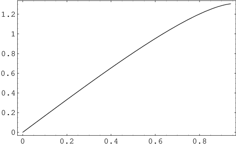
As shown in [8, 9], thermodynamically stable black hole embeddings for the D7-branes exist for , or equivalently for , and in this parameter range is a monotonically increasing function of , as exhibited in fig. 5. For or the free energy of the D7-branes is minimised by a Minkowski embedding, and so a first order phase transition occurs. Black hole embeddings with , or equivalently with , are expected to be metastable [21, 22], whereas those with have negative specific heat and are therefore unstable [9].
Converting the differential emission rate (3) to the emission rate per unit photon energy and using (40) gives
| (47) |
Our results for the spectral function and for the photon emission rate for thermodynamically stable black hole embeddings are shown in figs. 3, 4, and 6. Some interesting features of these plots are as follows.

|

|
The top, solid, red curve in fig. 3 corresponds to the analytic result (45) for massless quarks. This is a monotonically decreasing function that for large frequencies decays as . All curves with are also monotonically decreasing functions of the frequency, whereas curves with are increasing functions of for small . At large values of all curves seem to decay with the same power of the frequency as the curve, presumably due to the fact that at large the scale associated to the quark mass becomes irrelevant. The behaviour at small can also be easily understood. As the suppression factor in eq. (40) dominates, and so for small values of the spectral density decreases monotonically with , as shown in fig. 4. This effect is also responsible for the fact that the height of the peak of the photon emission curves in fig. 6 largely decreases as increases from zero to its maximum value. The suppression factor above has a simple geometric origin as the decreasing area of the induced black hole horizon on the D7-branes as increases, as can be seen from eq. (29).
Note that the top, solid, red curve in fig. 4, which corresponds to , gives (up to normalisation) the electric conductivity (10). Specifically, denoting by the curve in question, one has:
| (48) |
Again, the difference between our scaling and the scaling found in [6] reflects the difference in the number of electrically charged degrees of freedom.
At intermediate values of the spectral function is not a monotonic function of , as can be seen in fig. 4. In fig. 3 this is reflected in the fact that curves for different values of cross each other around . The same behaviour is of course observed in the plot of the photon production shown in fig. 6.
It is also interesting to examine the spectral function for black hole embeddings beyond the phase transition, i.e., in the region in which these embeddings are metastable or unstable. The results for the spectral function are shown in fig. 7. The most remarkable feature of these plots is the appearance of well defined peaks in the spectral function, which become narrower and more closely spaced, seemingly approaching delta-functions, as . We will discuss the interpretation of this fact in the last section.

5 The D4/D6 system
We now turn to the D4/D6 system, described by the array
| (49) |
In the decoupling limit, the resulting gauge theory is five-dimensional SYM coupled to fundamental hypermultiplets confined to a four-dimensional defect, so we have again . In order to obtain a four-dimensional gauge theory at low energies, one may compactify , the D4-brane direction orthogonal to the defect, on a circle. If periodic boundary conditions for the adjoint fermions are imposed, then supersymmetry is preserved and the four-dimensional theory thus obtained is non-confining. In this case the appropriate dual gravitational background at any temperature is (3) with periodically identified. Instead, if antiperiodic boundary conditions for the adjoint fermions are imposed, then supersymmetry is broken and the four-dimensional theory exhibits confinement [12] and spontaneous chiral symmetry breaking [14]. The holographic description at zero-temperature consists then of D6-brane probes in a horizon-free background, whose precise form is not needed here. At a temperature set by the radius of compactification, the theory undergoes a first order phase transition at which the gluons and the adjoint matter become deconfined. In the dual description the low-temperature background is replaced by (3). If , the D6-branes remain outside the horizon in a Minkowski embedding. As is further increased up to a first order phase transition for the fundamental matter occurs.
The metric (3) for the black D4-brane is
| (50) |
where
| (51) |
The five-dimensional Yang-Mills coupling constant in the dual gauge theory is dimensionful and given by . It is convenient to introduce the dimensionless coordinate , in terms of which the metric becomes
| (52) |
with . As before, the horizon is at and the boundary at .55 5 The D4-brane metric considered in this section is not asymptotically of the form times a sphere. The framework for the calculation of correlators is less well developed for such backgrounds, so we will proceed by analogy with the case. Presumably, however, this procedure can be made rigourous by lifting the D4-brane geometry to M-theory, in which it becomes an M5-brane geometry whose asymptotic form is . The D6-brane lifts in turn to a KK-monopole, whose worldvolume effective action can be found in [29]. Since the D6-branes wrap a two-sphere in the directions transverse to the D4-branes, it is also useful to write the metric on the four-sphere as
| (53) |
and to set . The D6-brane embedding is then specified as , in terms of which the induced metric takes the form
| (54) |
In eqs. (50) and (52) , whereas in (54) and all equations below in this section .
As in the previous section, the branes embedding is determined by extremising the action (16) with . Note that in this case there is a non-constant dilaton,
| (55) |
reflecting the non-conformality of the dual gauge theory. Near the boundary,66 6 In this limit, the coordinate used here and the coordinate used in [8, 9] are related through . behaves as
| (56) |
where the dimensionless constants and are proportional to the quark mass and condensate, respectively [8, 9]:
| (57) | |||||
| (58) |
with
| (59) |
the effective ’t Hooft coupling at the scale . In this case, we may write with
| (60) |
The scale is again related to the mass gap in the meson spectrum of the D4/D6 system at zero temperature through [20].
Following the previous section one obtains the equation of motion (21) with the functions given in this case by
| (61) |
This equation of motion may be derived from the action (22), where
| (62) |
and
| (63) |
is the normalisation constant introduced in [8, 9]. In this case eq. (39) becomes
| (64) |
and the trace of the spectral density, eq. (8), takes the form
| (65) |
The action (16) for the D6-branes in the absence of a gauge field reduces to
| (66) |
From this point one proceeds in complete analogy with the D3/D7 system, i.e., one solves for the D6-brane embedding numerically and uses the result to solve, also numerically, for the function . Substituting this in (65) one obtains the trace of the spectral density.
In this case the phase transition takes place at or . Below these values black hole embeddings are stable, whereas for , or , they are presumably metastable. For black hole embeddings possess a negative specific heat and are therefore unstable [9]. The results for stable embeddings are plotted in figs. 8, 9 and 10, whereas those for metastable or unstable embeddings are shown in fig. 11. Remarkably, these plots share many of the qualitative features of the D3/D7 system. We will come back to this in the next section.


|

|

6 Discussion
Results from heavy ion collision experiments at RHIC indicate that the QGP created there behaves as a strongly coupled liquid. In the absence of systematic, non-perturbative methods to calculate real-time observables in QCD, it is useful to calculate these observables in gauge theories for which a gravity dual is known, the hope being that universal properties of such theories may be shared by QCD itself.
In this paper we have calculated retarded correlators of electromagnetic currents at light-like momenta in a class of large-, strongly coupled SYM theories with flavours of fundamental matter. From these correlators one may extract several observables associated to photon production. Our results are valid to leading order in the electromagnetic coupling constant and in , but non-perturbatively in the interactions. At a qualitative level, these results exhibit a number of universal features.
For small values of the quark mass the combination is a featureless, monotonically decreasing function of , as observed in figs. 3 and 8. Instead, for large enough values of , first increases with , then reaches a maximum and finally decays as for large . The exponent is however not universal: For the D3/D7 system one has , whereas for the D4/D6 one finds .
The qualitative behaviour of as a function of for fixed values of also exhibits universal features. For small this is a monotonically decreasing function of , as displayed in figs. 4 and 9; in particular, the top, solid, red curves in these figures, which correspond to , yield (up to normalisation) the electric conductivity.77 7 In the D4/D6 system the electric conductivity is , where is the top, solid, red curve in fig. 9. Instead, for intermediate values of , the spectral function as a function of ceases to be monotonic. In figs. 3 and 8 this is reflected in the fact that curves for different values of cross each other. This is also the case for the photon production curves, as can be seen in figs. 6 and 10. This is perhaps a counterintuitive result, as it means that, at certain frequencies, plasmas with heavier quarks glow more brightly than those with lighter quarks.
Above we have calculated the rate of photon emission of an homogeneous, infinitely extended, thermally equilibrated plasma. In order to extract a prediction for a physical situation such as that of a heavy ion collision experiment, our results would have to be integrated over the spacetime evolution of the plasma created in such experiments, as determined by some hydrodynamic model [30]. In such a situation the temperature changes over time (and space) from some initial, maximum temperature , to some final, minimum temperature , and one measures the total number of produced photons of a given energy. This means that, unlike in the plots presented above, both and vary simultaneously as and (for the D3/D7 system) or (for the D4/D6 system). Temperatures around are expected to be achieved at LHC, whereas those at RHIC are roughly around , where MeV is the deconfinement temperature in QCD. On the other hand, is the lowest temperature for which a plasma description is appropriate, since below such a temperature hadronisation occurs. For illustrative purposes, let us therefore consider the photon emission predicted by our models as a function of , for and for fixed values of and . It is then convenient to write
| (67) |
Additionally, for the D3/D7 system we have
| (68) |
whereas for the D4/D6 system
| (69) |
Recall that is the typical mesonic scale in the gauge theory at zero temperature.
We are interested in the rate of photon production as varies between 1/4 and 1 for fixed values of . Converting the differential emission rate (3) to the emission rate per unit photon energy and using the results (40), (65) for the spectral functions gives
| (70) |
where for the D3/D7 system, for the D4/D6 system, and the factor must be understood as a function of .
The right-hand side of eq. (70) for the D3/D7 system is plotted in fig. 13 for several values of the photon energy and the mesonic scale . Specifically, the top graph corresponds to MeV, whereas the bottom graph corresponds to MeV. The meson masses correspond to representative values in QCD for bound states of and quarks, quarks and quarks: . For comparison, we have also included curves for and , where MeV is the critical mass (corresponding to ) for which the phase transition to a Minkowski embedding takes place exactly at . For this transition takes place at , and this is the reason why the dotted, orange curve terminates at : At this temperature the corresponding quarks form mesonic bound states, i.e., in the string description the probe D7-branes jump from a black hole to a Minkowski embedding.

|

|
Fig. 14 displays an analogous plot for the D4/D6 system, for MeV. In this case the dashed, green line also terminates at , since for the D4/D6 system both the and the mesons survive as bound states above the deconfinement temperature [9].

One common feature of both models is that the rate of photon production is most sensitive to the quark mass for low-energy photons and low temperatures. As we see in fig. 13, the difference between the curves is greater for MeV than for MeV, and in the former case it is greater for low temperatures. We have verified that as increases above 1000 MeV, the difference between curves becomes smaller and smaller. The same conclusion holds for the D4/D6 system. It is also remarkable that, contrary to what one might have perhaps expected, the rate of photon production associated to heavier quarks is smaller than that of lighter quarks, but it is not negligibly smaller. For example, we see in the figs. above that the number of photons emitted by quarks is a significant fraction of the number of photons emitted by and quarks for a wide range of temperatures.
Before leaving our discussion of possible implications for heavy ion collision experiments, we would like to emphasise that our results apply to photons produced by a thermally equilibrated plasma. However, in heavy ion collisions there are other sources of photon production. For example, prompt photons are produced by initial collisions of the partons that constitute the colliding ions, whereas decay photons are produced by the decay of certain hadrons once the plasma ball has hadronised. Thus comparison of any theoretical prediction for thermal photons to empirical data requires being able to distinguish experimentally between these different sources.
The features described above refer to thermodynamically stable black hole embeddings, but we also obtained results for metastable and unstable embeddings. These embeddings are skipped over by the meson-melting phase transition, but they are still interesting since they illustrate how the spectral function approaches that of Minkowski embeddings, as discussed in [22]. Results for the spectral function for several near-critical embeddings, i.e., for values of close to 1, are displayed in figs. 7 and 11. Clearly the spectral function develops closely spaced, narrow peaks that seemingly approach delta-functions. Thus the form of the spectral function appears to approach the form we expect for Minkowski embeddings,88 8 An analogous result was found in [22] for time-like momenta. namely an infinite sum of delta functions supported at a discrete set of energies . Each of these delta-functions is associated to a meson mode on the Dq-branes with null momentum. The existence of these modes may seem surprising in view of the fact that, as expected on general grounds and as verified in ref. [9], the meson spectrum in the Minkowski phase possesses a mass gap, but in fact it follows from the analysis in ref. [9]. To see this, consider the dispersion relation for a given meson in the Minkowski phase. The fact that there is a mass gap means that at . On the other hand, in the limit of infinite spatial momentum, , the dispersion relation takes the form with . The reason for this is easily understood: For larger and larger spatial momenta, the wave function of the meson becomes more and more concentrated at the tip of the Dq-branes, and so the speed of the meson is simply the local speed of light at this lowest point. Because of the gravitational redshift, this speed is always subluminal. Continuity then implies that there must exist a value of such that .

This is illustrated by the fact that the solid black line in fig. 15 intersects the other two curves. Although the curves shown in the fig. 15 correspond to scalar mesons, it is clear from the arguments above that an analogous result would hold for other types of mesons, in particular for vector-like mesons. Since these mesons are absolutely stable in the large-, strong coupling limit under consideration, they give rise to delta-function-like (i.e., zero-width) peaks in the spectral function of electromagnetic currents.
In this paper we have studied photon production by calculating the electromagnetic current-current correlator (5) at light-like momenta. It would be interesting to extend the calculation to time-like momenta, since this determines the nuumber of dileptons produced by virtual photon decay. A first step in this direction was given in ref. [22], where the correlator was calculated for vanishing spatial momentum.
A further extension consists of calculating the rate of photon and dilepton production in the presence of a finite baryon chemical potential [31, 32] of density [28, 33]. For non-zero baryon density black hole embeddings exist for all values of and , and so for large the spectral function of electromagnetic currents should again reveal high and narrow peaks corresponding to the existence in the spectrum of long-lived vector mesons [32].
Acknowledgments.
It is a pleasure to thank S. Hartnoll, P. Kovtun, R. Myers, D.T. Son, A. Starinets and L. Yaffe for helpful discussions. We are also grateful to R. Myers for a careful reading of this manuscript, and to the authors of [22] for sharing their work with us prior to publication. DM acknowledges support from NSF grant No PHY-0555669. LP acknowledges support from NSF grant No PHY03-54978 and from PROFIP (UNAM, Mexico).References
- [1] P. Stankus, “Direct photon production in relativistic heavy-ion collisions,” Ann. Rev. Nucl. Part. Sci. 55, 517 (2005).
- [2] See [3] for a complete result at leading order, and references therein for previous calculations.
- [3] P. Arnold, G. D. Moore and L. G. Yaffe, “Photon emission from ultrarelativistic plasmas,” JHEP 0111, 057 (2001) [arXiv:hep-ph/0109064]; “Photon emission from quark gluon plasma: Complete leading order results,” JHEP 0112, 009 (2001) [arXiv:hep-ph/0111107].
- [4]
E. Shuryak,
“Why does the quark gluon plasma at RHIC behave as a nearly ideal fluid?,”
Prog. Part. Nucl. Phys. 53, 273 (2004)
[arXiv:hep-ph/0312227];
D. Teaney, “Effect of shear viscosity on spectra, elliptic flow, and Hanbury Brown-Twiss radii,” Phys. Rev. C 68, 034913 (2003) [arXiv:nucl-th/0301099]. - [5] J. M. Maldacena, “The large N limit of superconformal field theories and supergravity,” Adv. Theor. Math. Phys. 2, 231 (1998) [Int. J. Theor. Phys. 38, 1113 (1999)] [arXiv:hep-th/9711200].
- [6] S. Caron-Huot, P. Kovtun, G. D. Moore, A. Starinets and L. G. Yaffe, “Photon and dilepton production in supersymmetric Yang-Mills plasma,” JHEP 0612, 015 (2006) [arXiv:hep-th/0607237].
- [7] A. Parnachev and D. A. Sahakyan, “Photoemission with chemical potential from QCD gravity dual,” Nucl. Phys. B 768, 177 (2007) [arXiv:hep-th/0610247].
- [8] D. Mateos, R. C. Myers and R. M. Thomson, “Holographic phase transitions with fundamental matter,” Phys. Rev. Lett. 97, 091601 (2006) [arXiv:hep-th/0605046].
- [9] D. Mateos, R. C. Myers and R. M. Thomson, “Thermodynamics of the brane,” JHEP 0705, 067 (2007) [arXiv:hep-th/0701132].
- [10] D. Mateos, R. C. Myers and R. M. Thomson, “Holographic viscosity of fundamental matter,” Phys. Rev. Lett. 98, 101601 (2007) [arXiv:hep-th/0610184].
- [11]
A. Karch and L. Randall,
“Open and closed string interpretation of SUSY CFT’s on branes with
boundaries,”
JHEP 0106, 063 (2001)
[arXiv:hep-th/0105132];
A. Karch and E. Katz, “Adding flavor to AdS/CFT,” JHEP 0206, 043 (2002) [arXiv:hep-th/0205236]. - [12] E. Witten, “Anti-de Sitter space, thermal phase transition, and confinement in gauge theories,” Adv. Theor. Math. Phys. 2 (1998) 505 [arXiv:hep-th/9803131].
- [13]
J. Babington, J. Erdmenger, N.J. Evans, Z. Guralnik and I. Kirsch,
“Chiral symmetry breaking and pions in non-supersymmetric
gauge/gravity duals,” Phys. Rev. D 69 (2004) 066007
[arXiv:hep-th/0306018];
I. Kirsch, “Generalizations of the AdS/CFT correspondence,” Fortsch. Phys. 52 (2004) 727 [arXiv:hep-th/0406274].
- [14] M. Kruczenski, D. Mateos, R.C. Myers and D.J. Winters, “Towards a holographic dual of large- QCD,” JHEP 0405 (2004) 041 [arXiv:hep-th/0311270].
- [15]
T. Albash, V. Filev, C.V. Johnson and A. Kundu, “A
topology-changing phase transition and the dynamics of flavour,”
arXiv:hep-th/0605088;
T. Albash, V. Filev, C.V. Johnson and A. Kundu, “Global currents, phase transitions, and chiral symmetry breaking in large gauge theory,” arXiv:hep-th/0605175;
- [16] A. Karch and A. O’Bannon, “Chiral transition of N=4 super Yang-Mills with flavor on a 3-sphere,” Phys. Rev. D 74 (2006) 085033 [arXiv:hep-th/0605120].
- [17]
O. Aharony, J. Sonnenschein and S. Yankielowicz,
“A holographic model of deconfinement and chiral symmetry restoration,”
Annals Phys. 322, 1420 (2007)
[arXiv:hep-th/0604161];
A. Parnachev and D.A. Sahakyan, “Chiral phase transition from string theory,” Phys. Rev. Lett. 97 (2006) 111601 [arXiv:hep-th/0604173];
Y.H. Gao, W.S. Xu and D.F. Zeng, “NGN, QCD2 and chiral phase transition from string theory,” JHEP 0608 (2006) 018 [arXiv:hep-th/0605138];
E. Antonyan, J.A. Harvey and D. Kutasov, “The Gross-Neveu model from string theory,” arXiv:hep-th/0608149. - [18] M. Kruczenski, D. Mateos, R.C. Myers and D.J. Winters, “Meson spectroscopy in AdS/CFT with flavour,” JHEP 0307 (2003) 049 [arXiv:hep-th/0304032].
- [19]
D. Arean and A.V. Ramallo, “Open string modes at brane
intersections,” JHEP 0604 (2006) 037
[arXiv:hep-th/0602174];
A.V. Ramallo, “Adding open string modes to the gauge/gravity correspondence,” Mod. Phys. Lett. A 21 (2006) 1481 [arXiv:hep-th/0605261]. - [20] R.C. Myers and R.M. Thomson, “Holographic mesons in various dimensions,” JHEP 0609 (2006) 066 [arXiv:hep-th/0605017].
- [21] C. Hoyos, K. Landsteiner and S. Montero, “Holographic meson melting,” JHEP 0704, 031 (2007) [arXiv:hep-th/0612169].
- [22] R. C. Myers, A. O. Starinets and R. M. Thomson, “Holographic spectral functions and diffusion constants for fundamental matter,” arXiv:0706.0162 [hep-th].
- [23] See for example M. Le Bellac, “Thermal Field Theory”, Cambridge, 1996.
- [24] E. Witten, “Anti-de Sitter space and holography,” Adv. Theor. Math. Phys. 2, 253 (1998) [arXiv:hep-th/9802150].
- [25] G. Policastro, D. T. Son and A. O. Starinets, “From AdS/CFT correspondence to hydrodynamics,” JHEP 0209, 043 (2002) [arXiv:hep-th/0205052].
- [26] D.T. Son and A.O. Starinets, “Minkowski-space correlators in AdS/CFT correspondence: Recipe and applications,” JHEP 0209 (2002) 042 [arXiv:hep-th/0205051].
- [27] C.P. Herzog and D.T. Son, “Schwinger-Keldysh propagators from AdS/CFT correspondence,” JHEP 0303 (2003) 046 [arXiv:hep-th/0212072].
- [28] S. Kobayashi, D. Mateos, S. Matsuura, R. C. Myers and R. M. Thomson, “Holographic phase transitions at finite baryon density,” JHEP 0702, 016 (2007) [arXiv:hep-th/0611099].
- [29] E. Bergshoeff, B. Janssen and T. Ortin, “Kaluza-Klein monopoles and gauged sigma-models,” Phys. Lett. B 410, 131 (1997) [arXiv:hep-th/9706117].
- [30] See e.g., P. Huovinen and P. V. Ruuskanen, “Hydrodynamic models for heavy ion collisions,” Ann. Rev. Nucl. Part. Sci. 56, 163 (2006) [arXiv:nucl-th/0605008], and references therein.
- [31] S. Nakamura, Y. Seo, S.J. Sin and K.P. Yogendran, “Baryon-charge Chemical Potential in AdS/CFT,” arXiv:0708.2818 [hep-th]; K. Ghoroku, M. Ishihara and A. Nakamura, “D3/D7 holographic Gauge theory and Chemical potential,” arXiv:0708.3706 [hep-th]; A. Karch and A. O’Bannon, “Holographic Thermodynamics at Finite Baryon Density: Some Exact Results,” arXiv:0709.0570 [hep-th].
- [32] D. Mateos, S. Matsuura, R. C. Myers and R. M. Thomson, “Holographic phase transitions at finite chemical potential,” arXiv:0709.1225 [hep-th].
- [33] S. Nakamura, Y. Seo, S.J. Sin and K.P. Yogendran, “A New Phase at Finite Quark Density from AdS/CFT,” arXiv:hep-th/0611021.