Dynamical response functions in the quantum Ising chain with a boundary

Over the last decade there has been significant progress in the calculation of dynamical correlation functions in integrable quantum field theories Smirnov92book; fring93; Lukyanov95; lukyanov; babujian; Delfino04. This has made it possible to determine the dynamic response of a variety of experimentally relevant one-dimensional models of Ising magnets DelfinoMussardo95; CarrTsvelik03, integer applSint; Konik03 and spin-1/2 applShalf quantum magnets, Mott insulators applMI, two-leg ladders appl2leg, carbon nanotubes applnano and ultra-cold atomic gases applgas. Having established the bulk behaviour of such systems, it is of interest to investigate the effects of impurities on the dynamic response. The simplest possible effect of non-magnetic impurities in a spin chain material is to break the chains into finite segments. Resulting changes in the susceptibility have been investigated in both spin-1/2 affleck and spin-1 edgestates Heisenberg chains as well as two-leg Heisenberg ladders ladder. In the latter two cases the chain break can lead to the formation of edge states, which have been observed in inelastic neutron scattering experiments edgestates2. Impurity and boundary effects are also relevant to scanning tunneling microscopy experiments STM, where the associated breaking of translational symmetry can lead to fingerprints in the dynamic response that assist in characterising of the underlying bulk behaviour Kivelson. For the aforementioned reasons it is important to extend the calculation of dynamical response functions in one-dimensional models to systems with boundaries. In the gapless case this is readily accomplished by boundary conformal field theory Cardy84; Cardy89, while the gapful case is as usual more involved. One successful approach has been the extension of the truncated conformal space approach TCSA to systems with boundary Dorey-98; Dorey-01. The method we will follow in the present work is the extension of the form factor bootstrap approach to boundary integrable field theories GhoshalZamolodchikov94; FringKoeberle94; Konik-96; BajnokGeorge06; Bajnok-07. We will focus on the simplest integrable field theory, the quantum Ising chain Onsager44; McCoyWu73; ising1; Berg-79; Bariev; CardyMussardo90; YurovZamolodchikov91; Delfino04. One-point functions in the boundary Ising model have been studied by Konik et al. Konik-96. The purpose of the present work is to analyse two-point functions relevant to scattering experiments.

This article is organised as follows. First, we will review the basic facts on the Ising field theory in the bulk. We proceed by discussing the Ising model on the half line in the presence of a boundary magnetic field and the form factor bootstrap approach to boundary integrable field theories. In order to set the stage, we calculate the Green’s functions of the Majorana fermions, which show typical light-cone effects. After a brief discussion of the local magnetisation we proceed with our main result, the calculation of the dynamical spin-spin correlations and the corresponding spectral function. The derived expansion in terms of infinite volume form factors and a boundary state is found to be rapidly convergent as long as $|\frac{x_{1}+x_{2}}{\xi}|\gtrsim 0.2$ where $\xi$ is the correlation length. As for the Green’s functions we observe light-cone effects, which result in oscillatory behaviour of the correlations arbitrarily far away from the boundary. Furthermore, we study the effects of the boundary bound state, which exists for sufficiently small values of the boundary magnetic field, on the correlation function. Finally, we discuss the two-point function of the disorder field, which shows the same qualitative features as the spin-spin correlations.

The Hamiltonian of one-dimensional quantum Ising model is given by

$$H_{\mathrm{latt}}=-J\sum_{i}\bigl(\sigma^{\mathrm{z}}_{i}\,\sigma^{\mathrm{z}}_{i+1}+\lambda\,\sigma^{\mathrm{x}}_{i}\bigr).$$

(1)

Here $\sigma^{\mathrm{x}}$ and $\sigma^{\mathrm{z}}$ are the Pauli matrices and $J$ is the exchange energy. The model (1) is related to the two-dimensional classical Ising model, see for example Ref. GogolinNersesyanTsvelik98. The critical temperature of the latter is related to the coupling constant of the quantum Ising chain by $\lambda=\frac{T-T_{\mathrm{c}}}{T_{\mathrm{c}}}$. The Hamiltonian (1) is invariant under the $\mathbb{Z}_{2}$-transformation $\sigma_{i}^{\mathrm{x}}\rightarrow\sigma_{i}^{\mathrm{x}}$, $\sigma_{i}^{\mathrm{z}}\rightarrow-\sigma_{i}^{\mathrm{z}}$. For $\lambda<1$, which corresponds to the low-temperature phase of the 2D classical Ising model, this symmetry is broken. The order parameter field $\sigma_{i}^{\mathrm{z}}$ takes a non-zero expectation value and the ground state is two-fold degenerate. For $\lambda>1$ the model has a unique ground state. This regime corresponds to the disordered high-temperature phase of the classical 2D Ising model. The point $\lambda=1$ is the location of a quantum phase transition.

At small deviations from criticality, $|\lambda-1|\ll 1$, one can pass to the continuum limit ItzyksonDrouffe89vol1; GogolinNersesyanTsvelik98. This leads to the Ising field theory, which is defined by the Euclidean action ItzyksonDrouffe89vol1; Delfino04

$$\mathcal{S}=\frac{1}{2\pi}\int d^{2}x\left(\psi\bar{\partial}\psi+\bar{\psi}\partial\bar{\psi}+\text{i}\,M\bar{\psi}\psi\right),$$

(2)

where $\psi$ and $\bar{\psi}$ are the two components of a Majorana fermion. The complex coordinates used in (2) are given by $z=\tau+\text{i}\,x$ and $\bar{z}=\tau-\text{i}\,x$, where $\tau=\text{i}\,t$ denotes imaginary time. This results in $\partial=\partial_{z}=(\partial_{\tau}-\text{i}\,\partial_{x})/2$ and $\bar{\partial}=\partial_{\bar{z}}=(\partial_{\tau}+\text{i}\,\partial_{x})/2$. The mass is proportional to the distance from the critical point, $M\propto J(1-\lambda)$. The model (2) is conformally invariant at the critical point $M=0$ (see for example Ref. DiFrancescoMathieuSenechal97). In the ordered phase, which we will consider throughout this paper, the mass is positive. Furthermore, we set the velocity to one and use the short distance normalisations

$$z\left\langle 0\right|\psi(\tau,x)\,\psi(0,0)\left|0\right\rangle\rightarrow 1,\quad|z|^{1/4}\left\langle 0\right|\sigma^{\mathrm{z}}(\tau,x)\,\sigma^{\mathrm{z}}(0,0)\left|0\right\rangle\rightarrow 1,\quad\text{as}\quad|z|\rightarrow 0.$$

(3)

For later use we will need the notion of mutual semi-locality of operators YurovZamolodchikov91; Smirnov92book; Lukyanov95; Delfino04. Let us consider the operator product $O_{1}(\tau,x)\,O_{2}(0,0)=O_{1}(z,\bar{z})\,O_{2}(0,0)$. If we take $O_{1}$ counterclockwise around $O_{2}$ in the plane, i.e., we perform the analytic continuation $z\rightarrow e^{2\pi\text{i}\,}z$, $\bar{z}\rightarrow e^{-2\pi\text{i}\,}\bar{z}$, the operators $O_{1}$ and $O_{2}$ are said to be mutually semi-local if

$$O_{1}(e^{2\pi\text{i}\,}z,e^{-2\pi\text{i}\,}\bar{z})\,O_{2}(0,0)=l_{O_{1}O_{2}}\,O_{1}(z,\bar{z})\,O_{2}(0,0).$$

(4)

The phase $l_{O_{1}O_{2}}$ is called the semi-locality factor. The two fields are mutually local if $l_{O_{1}O_{2}}=1$. Semi-locality is the mildest form of non-locality, in general the right-hand side of (4) may be more complicated. The mutual semi-locality factor of the spin and disorder operators can be read off from their operator product expansion DiFrancescoMathieuSenechal97; Delfino04

$$\sigma^{\mathrm{z}}(z,\bar{z})\,\mu^{\mathrm{z}}(0,0)\sim\frac{1}{\sqrt{2}\,|z|^{1/4}}\,\bigl(e^{\text{i}\,\pi/4}\sqrt{z}\,\psi(0)+e^{-\text{i}\,\pi/4}\sqrt{\bar{z}}\,\bar{\psi}(0)\bigr).$$

(5)

This implies that when taking $\sigma^{\mathrm{z}}$ once around $\mu^{\mathrm{z}}$ one obtains an extra minus sign, i.e., $l_{\sigma^{\mathrm{z}}\mu^{\mathrm{z}}}=-1$. In the same way one finds $l_{\psi\mu^{\mathrm{z}}}=l_{\bar{\psi}\mu^{\mathrm{z}}}=l_{\psi\sigma^{\mathrm{z}}}=l_{\bar{\psi}\sigma^{\mathrm{z}}}=-1$. On the other hand, the disorder field $\mu^{\mathrm{z}}$ is local with respect to itself.

In order proceed further, we need to construct a basis of scattering states. In order to do so, we need to specify which “fundamental field” (that is a field that has a non-vanishing matrix element between the vacuum and the one-particle states) we will use to create the fundamental excitations. In order to avoid additional signs in many of the equations it is customary to choose the fundamental field to be bosonic. We will therefore use the disorder field $\mu^{\mathrm{z}}$. This implies that the fundamental excitations are viewed as bosons with two-particle scattering matrix $S=-1$. Let us denote the corresponding annihilation and creation operators by $A(\theta)$ and $A^{\dagger}(\theta)$ respectively. They fulfil the Faddeev–Zamolodchikov algebra

	$\displaystyle A(\theta_{1})A(\theta_{2})$	$\displaystyle=$	$\displaystyle SA(\theta_{2})A(\theta_{1}),$
	$\displaystyle A^{\dagger}(\theta_{1})A^{\dagger}(\theta_{2})$	$\displaystyle=$	$\displaystyle SA^{\dagger}(\theta_{2})A^{\dagger}(\theta_{1}),$		(6)
	$\displaystyle A(\theta_{1})A^{\dagger}(\theta_{2})$	$\displaystyle=$	$\displaystyle 2\pi\delta(\theta_{1}-\theta_{2})+SA^{\dagger}(\theta_{2})A(\theta_{1}),$

where the scattering matrix is $S=-1$. The vacuum state is then defined by

$$A(\theta)|0\rangle=0,$$

(7)

and a basis of scattering states is given as

$$\left|\theta_{1},\ldots,\theta_{n}\right\rangle=A^{\dagger}(\theta_{1})\ldots A^{\dagger}(\theta_{n})\left|0\right\rangle.$$

(8)

In terms of the states (8) the resolution of the identity reads

$$\mathrm{id}=\left|0\right\rangle\left\langle 0\right|+\sum_{n=1}^{\infty}\frac{1}{n!}\int_{-\infty}^{\infty}\frac{d\theta_{1}\ldots d\theta_{n}}{(2\pi)^{n}}\left|\theta_{1},\ldots,\theta_{n}\right\rangle\left\langle\theta_{n},\ldots,\theta_{1}\right|.$$

(9)

For the calculation of correlation functions the knowledge of the matrix elements or form factors of local operators is necessary. In the ordered phase the non-vanishing form factors of $\sigma^{\mathrm{z}}$ contain an even number of particles and are explicitly given by Berg-79; CardyMussardo90; YurovZamolodchikov91; Delfino04

$$f(\theta_{1},\ldots,\theta_{2n})=\left\langle 0\right|\sigma^{\mathrm{z}}(0,0)\left|\theta_{1},\ldots,\theta_{2n}\right\rangle=\text{i}\,^{n}\sigma_{0}\prod_{\begin{subarray}{c}i,j=1\\ i<j\end{subarray}}^{2n}\tanh\frac{\theta_{i}-\theta_{j}}{2},$$

(10)

where $\sigma_{0}=\left\langle 0\right|\sigma^{\mathrm{z}}\left|0\right\rangle$. For comparison, the form factors of the disorder operator $\mu^{\mathrm{z}}$ are only non-vanishing if the number of particles is odd,

$$\left\langle 0\right|\mu^{\mathrm{z}}(0,0)\left|\theta_{1},\ldots,\theta_{2n+1}\right\rangle=\text{i}\,^{n}\sigma_{0}\prod_{\begin{subarray}{c}i,j=1\\ i<j\end{subarray}}^{2n+1}\tanh\frac{\theta_{i}-\theta_{j}}{2}.$$

(11)

The form factors (10) and (11) follow from the following set of requirements Smirnov92book; Lukyanov95; Delfino04:

1. 1.

   The form factors $f(\theta_{1},\ldots,\theta_{n})$ are meromorphic functions of $\theta_{n}$ in the physical strip $0\leq\mathfrak{Im}\,\theta_{n}\leq 2\pi$. There exist only simple poles in this strip.

2. 2.

   Scattering axiom:

   $$f(\theta_{1},\ldots,\theta_{i+1},\theta_{i},\ldots,\theta_{n})=S\,f(\theta_{1},\ldots,\theta_{i},\theta_{i+1},\ldots,\theta_{n}),$$

   with the scattering matrix $S=-1$.

3. 3.

   Periodicity axiom:

   $$f(\theta_{1}+2\pi\text{i}\,,\theta_{2},\ldots,\theta_{n})=l_{O\mu^{\mathrm{z}}}\,f(\theta_{2},\ldots,\theta_{n},\theta_{1}),$$

   where $O=\sigma^{\mathrm{z}}$ or $\mu^{\mathrm{z}}$. The mutual non-locality phases are given by $l_{\sigma^{\mathrm{z}}\mu^{\mathrm{z}}}=-1$ and $l_{\mu^{\mathrm{z}}\mu^{\mathrm{z}}}=1$, respectively.

4. 4.

   Lorentz invariance:

   $$f(\theta_{1}+\alpha,\ldots,\theta_{n}+\alpha)=e^{s\alpha}\,f(\theta_{1},\ldots,\theta_{n}),$$

   where $s$ denotes the spin of the fields, which is $s_{\sigma^{\mathrm{z}}}=0$ and $s_{\mu^{\mathrm{z}}}=0$ as well as $s_{\psi}=-1/2$ and $s_{\bar{\psi}}=1/2$.

5. 5.

   Annihilation pole axiom:

   $$\mathrm{Res}\bigl[f(\theta^{\prime},\theta,\theta_{1},\ldots,\theta_{n}),\theta^{\prime}=\theta+\text{i}\,\pi\bigr]=\text{i}\,f(\theta_{1},\ldots,\theta_{n})\left[1-l_{O\mu^{\mathrm{z}}}\prod\nolimits_{i=1}^{n}S\right].$$

   Note that the squared brackets on right-hand side equal $2$ for $\sigma^{\mathrm{z}}$ as well as $\mu^{\mathrm{z}}$, as the extra minus sign due to $l_{\sigma^{\mathrm{z}}\mu^{\mathrm{z}}}=-1$ is compensated by an additional factor $S$. As there exist no bound states in the Ising model, these are the only poles of the form factors.

We note that if we had used the Majorana fermion $\psi$ as fundamental field, the excitations would be viewed as fermions with unity scattering matrix. Furthermore, there would appear additional minus signs in the axioms above YurovZamolodchikov91.

We now turn to the Ising field theory on the half-plane $(\tau,x)$, $\tau\in\mathbb{R}$, $x\in(-\infty,0]$. The boundary is located at $x=0$ and $\tau$ denotes imaginary time ($\tau=\text{i}\,t$). The Hilbert space of states associated with the semi-infinite line $\tau=\text{const.}$, $-\infty<x\leq 0$, is denoted by $\mathcal{H}_{\mathrm{B}}$. The boundary condition is imposed through application of an external time-independent magnetic field $h$ which couples to the boundary spin $\sigma_{\mathrm{b}}^{\mathrm{z}}(\tau)=\sigma^{\mathrm{z}}(\tau,0)$. The action for this system is given by GhoshalZamolodchikov94

$$\mathcal{S}=\frac{1}{2\pi}\int d\tau\int_{-\infty}^{0}dx\left(\psi\bar{\partial}\psi+\bar{\psi}\partial\bar{\psi}+\text{i}\,M\bar{\psi}\psi\right)+\frac{1}{2\pi}\int d\tau\left(h\sigma_{\mathrm{b}}^{\mathrm{z}}-\frac{\text{i}\,}{2}\bar{\psi}\psi-\frac{1}{2}\,a\,\partial_{\tau}a\right).$$

(12)

It was shown by Affleck and Ludwig AffleckLudwig91 that in the critical model the application a magnetic field at the boundary generates a flow from free to fixed boundary conditions. The properties of the boundary spin operator $\sigma_{\mathrm{b}}^{\mathrm{z}}$ were analysed in Refs Cardy89; CardyLewellen91. In the Lagrangian framework defined by (12) it can be written as GhoshalZamolodchikov94

$$\sigma_{\mathrm{b}}^{\mathrm{z}}(\tau)=\frac{1}{2}\bigl(\psi(\tau,x)+\bar{\psi}(\tau,x)\bigr)\Big|_{x=0}\,a(\tau).$$

(13)

Here $a(\tau)$ is an additional fermionic boundary degree of freedom which is introduced to describe the ground-state degeneracy and anticommutes with $\psi$ and $\bar{\psi}$. The cases $h=0$ and $h\rightarrow\infty$ correspond to free and fixed boundary conditions, respectively. We note that the application of a non-zero boundary magnetic field removes the ground-state degeneracy of the Ising model.

In terms of the Majorana fermions the boundary condition reads

$$-\text{i}\,\frac{d}{d\tau}\bigl(\psi-\bar{\psi}\bigr)\Big|_{x=0}=\frac{h^{2}}{2}\bigl(\psi+\bar{\psi}\bigr)\Big|_{x=0}.$$

(14)

As was shown by Ghoshal and Zamolodchikov GhoshalZamolodchikov94 the Ising model with boundary conditions (14) still possesses infinitely many integrals of motion (which can be constructed from the integrals of motion of the model in the bulk) and hence remains integrable.

If one thinks of the boundary as an infinitely heavy impenetrable particle $B$ sitting at $x=0$ and writes $\left|0_{\mathrm{B}}\right\rangle=B\left|0\right\rangle\in\mathcal{H}_{\mathrm{B}}$ for the ground state in the presence of the boundary, the scattering of particles created by the operators $A^{\dagger}(\theta)$ at the boundary is encoded in the relations

$$A^{\dagger}(\theta)B=R(\theta)A^{\dagger}(-\theta)B.$$

(15)

The function $R(\theta)$ is interpreted as the single-particle reflection amplitude off the boundary. In order to preserve the integrability of the corresponding bulk system, the boundary scattering matrix $R(\theta)$ has to satisfy several conditions as discussed in Ref. GhoshalZamolodchikov94, which leads to the following result for the boundary scattering matrix for the Ising model with boundary magnetic field $h$

$$R(\theta)=\text{i}\,\tanh\!\left(\frac{\text{i}\,\pi}{4}-\frac{\theta}{2}\right)\frac{\kappa-\text{i}\,\sinh\theta}{\kappa+\text{i}\,\sinh\theta},\quad\kappa=1-\frac{h^{2}}{2M}.$$

(16)

Free boundary conditions are recovered for $h=0$, whereas fixed boundary conditions are obtained in the limit $h\rightarrow\infty$ (we restrict ourselves to $h\geq 0$). The purpose of the present work is to calculate the two-point correlation function

$$C(\tau,x_{1},x_{2})=\left\langle 0_{\mathrm{B}}\right|\mathcal{T}_{\tau}\,\sigma^{\mathrm{z}}(\tau,x_{1})\,\sigma^{\mathrm{z}}(0,x_{2})\left|0_{\mathrm{B}}\right\rangle,$$

(17)

where $\mathcal{T}_{\tau}$ is the time-ordering operator. The time-dependence of the operators $\sigma^{\mathrm{z}}$ is given by

$$\sigma^{\mathrm{z}}(\tau,x)=e^{\tau H_{\mathrm{B}}}\,\sigma^{\mathrm{z}}(0,x)\,e^{-\tau H_{\mathrm{B}}},$$

(18)

where $H_{\mathrm{B}}$ is the Hamiltonian of the system in the presence of the boundary.

As we are working in the Euclidean formalism, $\tau$ and $x$ are interchangeable. Therefore, one may also take $x$ to be the Euclidean time, which implies that the equal-time section is the infinite line, $x=\text{const.}$, $-\infty<\tau<\infty$, and the associated Hilbert space $\mathcal{H}$ is that of the corresponding bulk theory (8). The boundary at $x=0$ now appears as an initial condition which is expressed in terms of a “boundary state” $\left|\mathrm{B}\right\rangle$. As was shown by Ghoshal and Zamolodchikov GhoshalZamolodchikov94, the correlation function (17) can then be expressed as

$$C(\tau,x_{1},x_{2})=\frac{\left\langle 0\right|\mathcal{T}_{x}\,\sigma^{\mathrm{z}}(\tau,x_{1})\,\sigma^{\mathrm{z}}(0,x_{2})\left|\mathrm{B}\right\rangle}{\left\langle 0\right|\mathrm{B}\rangle}.$$

(19)

Here $\mathcal{T}_{x}$ is the $x$-ordering operator, which orders the largest $x_{i}$ to the right, and $\left|0\right\rangle\in\mathcal{H}$ is the ground state of the model on the infinite line. The boundary state is given by

$$\left|\mathrm{B}\right\rangle=\exp\left(\int_{0}^{\infty}\frac{d\xi}{2\pi}K(\xi)A^{\dagger}(-\xi)A^{\dagger}(\xi)\right)\left|0\right\rangle,$$

(20)

where $K(\xi)=R(\text{i}\,\pi/2-\xi)$. For the Ising model it is explicitly given by

$$K(\xi)=\text{i}\,\tanh\frac{\xi}{2}\ \frac{\kappa+\cosh\xi}{\kappa-\cosh\xi}.$$

(21)

This simplifies to

$$K_{\mathrm{free}}(\xi)=-\text{i}\,\coth\frac{\xi}{2},\quad K_{\mathrm{fixed}}(\xi)=\text{i}\,\tanh\frac{\xi}{2},$$

(22)

for free and fixed boundary conditions, respectively. For later use we introduce the real function $\hat{K}(\xi)=-\text{i}\,K(\xi)$, which is plotted for several values of $\kappa$ in Fig. 3. We note that for $0\leq h\leq 2\sqrt{M}$ the function $\hat{K}(\xi)$ is negative for all $\xi$, whereas for $2\sqrt{M}<h$ the function $\hat{K}(\xi)$ is positive in a certain $\xi$-interval. Furthermore, for $0<h<h_{\mathrm{c}}=\sqrt{2M}$ one finds $\hat{K}(\xi)<-1$ for certain $\xi$. In this region the boundary scattering matrix (16) has a pole in the strip $0<\mathfrak{Im}\,\xi<\pi/2$, indicating the existence of a boundary bound state GhoshalZamolodchikov94. We will discuss this state in more detail in Sec. III.1 below. Finally, we note that for free boundary conditions the boundary scattering matrix (16) has a pole at $\xi=0$. This results in the appearance of a zero-momentum mode in the boundary state, i.e., (20) is replaced by GhoshalZamolodchikov94

$$\left|\mathrm{B_{free}}\right\rangle=\bigl(1+A^{\dagger}(0)\bigr)\exp\left(\int_{0}^{\infty}\frac{d\xi}{2\pi}K(\xi)A^{\dagger}(-\xi)A^{\dagger}(\xi)\right)\left|0\right\rangle.$$

(23)

Since all form factors of $\sigma^{\mathrm{z}}$ involving an odd number of particles vanish, this zero-momentum mode does not contribute to the two-point function (19) of $\sigma^{\mathrm{z}}$, and hence will be ignored in our analysis. Finally, we note that $K(\xi)=-K(-\xi)$ and $K(\xi)\rightarrow 0$ ($\xi\rightarrow 0$) except for free boundary conditions.

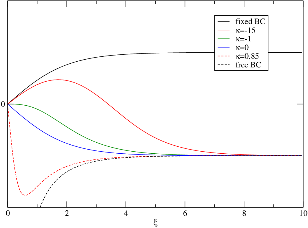
As we have interchanged space and time and $x$ is running from $0$ to $-\infty$ in the new framework, the $\tau$- and $x$-dependence of operators $\sigma^{\mathrm{z}}(\tau,x)$ is now given by

$$\sigma^{\mathrm{z}}(\tau,x)=e^{-xH}\,e^{-\text{i}\,\tau P}\,\sigma^{\mathrm{z}}(0,0)\,e^{\text{i}\,\tau P}\,e^{xH},$$

(24)

where $H$ is the Hamiltonian of the system on the infinite line, $-\infty<\tau<\infty$, and $P$ is the total momentum.

In order to set the stage, we first calculate the Green’s functions of the Majorana fermions. The mode expansions in the presence of the boundary and in the absence of a boundary bound state are given by

	$\displaystyle\psi(\tau,x)\!\!$	$\displaystyle=$	$\displaystyle\!\!\sqrt{\frac{M}{2}}\int\limits_{0}^{\infty}\!\frac{d\theta}{\sqrt{2\pi}}\,\biggl[c(\theta)\,e^{-\frac{\text{i}\,\pi}{4}}\,e^{-M\tau\cosh\theta}\Bigl(e^{-\frac{\theta}{2}}\,e^{\text{i}\,Mx\sinh\theta}+R(\theta)\,e^{\frac{\theta}{2}}\,e^{-\text{i}\,Mx\sinh\theta}\Bigr)$		(29)
			$\displaystyle\hskip 56.9055pt+c^{\dagger}(\theta)\,e^{\frac{\text{i}\,\pi}{4}}\,e^{M\tau\cosh\theta}\Bigl(e^{-\frac{\theta}{2}}\,e^{-\text{i}\,Mx\sinh\theta}+R(-\theta)\,e^{\frac{\theta}{2}}\,e^{\text{i}\,Mx\sinh\theta}\Bigr)\biggr],$
	$\displaystyle\bar{\psi}(\tau,x)\!\!$	$\displaystyle=$	$\displaystyle\!\!\sqrt{\frac{M}{2}}\int\limits_{0}^{\infty}\!\frac{d\theta}{\sqrt{2\pi}}\,\biggl[c(\theta)\,e^{\frac{\text{i}\,\pi}{4}}\,e^{-M\tau\cosh\theta}\left(e^{\frac{\theta}{2}}\,e^{\text{i}\,Mx\sinh\theta}+R(\theta)\,e^{-\frac{\theta}{2}}\,e^{-\text{i}\,Mx\sinh\theta}\right)$		(30)
			$\displaystyle\hskip 56.9055pt+c^{\dagger}(\theta)\,e^{-\frac{\text{i}\,\pi}{4}}\,e^{M\tau\cosh\theta}\Bigl(e^{\frac{\theta}{2}}\,e^{-\text{i}\,Mx\sinh\theta}+R(-\theta)\,e^{-\frac{\theta}{2}}\,e^{\text{i}\,Mx\sinh\theta}\Bigr)\biggr].$

Here $c(\theta)$ and $c^{\dagger}(\theta)$ are canonical fermion annihilation and creation operators $\{c(\theta),c^{\dagger}(\theta^{\prime})\}=2\pi\delta(\theta-\theta^{\prime})$.

The Green’s function of $\psi$ is now easily derived to be (we assume $\tau>0$ for simplicity)

$$\begin{split}\left\langle 0_{\mathrm{B}}\right|\psi(\tau,x_{1})\,\psi(0,x_{2})\left|0_{\mathrm{B}}\right\rangle&=\frac{M}{2}\int_{-\infty}^{\infty}d\theta\,e^{-M\tau\cosh\theta}\,\Bigl[e^{-\theta}\,e^{\text{i}\,Mr\sinh\theta}+R(\theta)\,e^{-2M\text{i}\,R\sinh\theta}\Bigr]\\[5.69054pt] &=M\sqrt{\frac{\text{i}\,\tau-r}{\text{i}\,\tau+r}}\,K_{1}\bigl(M\sqrt{r^{2}+\tau^{2}}\bigr)+\frac{M}{2}\int_{-\infty}^{\infty}d\theta\,R\bigl(\theta+\text{i}\,\theta_{0}\bigr)\,e^{-M\sqrt{4R^{2}+\tau^{2}}\cosh\theta},\end{split}$$

(31)

where $\theta_{0}=\arctan\bigl(2|R|/\tau\bigr)$ and $K_{1}$ denotes the modified Bessel function of order one AbramowitzStegun65. Furthermore, we have introduced centre-of-mass coordinates $R=(x_{1}+x_{2})/2$ and $r=x_{2}-x_{1}$. We stress that $R\leq 0$. In real space, $\tau=\text{i}\,t$, the first term is oscillating for $r^{2}<t^{2}$ and damped for $r^{2}>t^{2}$, i.e. we observe a light-cone effect. The second term is oscillating for $4R^{2}<t^{2}$ and damped otherwise. The physical interpretation of the oscillating behaviour is that for $4R^{2}<t^{2}$ a particle can propagate from $(0,x_{2})$ to $(t,x_{1})$ via the boundary (see Fig. 5). If one calculates the Green’s function using the rotated system and the boundary state, one obtains an additional phase of $\pi/2$. The physical origin of this phase is the Lorentz spin $s_{\psi}=-1/2$ of $\psi$, which implies that the Green’s function transforms non-trivial under Lorentz rotations. In the case $h<h_{\mathrm{c}}$ there is an additional term due to the presence of the boundary bound state.

In the same way one obtains (we assume $\tau>0$)

$$\left\langle 0_{\mathrm{B}}\right|\psi(\tau,x_{1})\,\bar{\psi}(0,x_{2})\left|0_{\mathrm{B}}\right\rangle=-\text{i}\,M\,K_{0}\bigl(M\sqrt{r^{2}+\tau^{2}}\bigr)-\text{i}\,\frac{M}{2}\sqrt{\frac{\text{i}\,\tau+2R}{\text{i}\,\tau-2R}}\,\int_{-\infty}^{\infty}d\theta\,R\bigl(\theta+\text{i}\,\theta_{0}\bigr)\,e^{\theta}\,e^{-M\sqrt{4R^{2}+\tau^{2}}\cosh\theta},$$

(32)

which shows the same kind of oscillatory behaviour as (31).

In this section we briefly discuss the one-point function of the spin operator. The one-point function in the ground state $\left|0_{\mathrm{B}}\right\rangle$ was first calculated by Konik, LeClair and Mussardo Konik-96 and to second order in $K$ is given by

$$\begin{split}\left\langle 0_{\mathrm{B}}\right|\sigma^{\mathrm{z}}(x)\left|0_{\mathrm{B}}\right\rangle&=\sigma_{0}-\text{i}\,\sigma_{0}\int_{0}^{\infty}\frac{d\xi}{2\pi}\,K(\xi)\,\tanh\xi\,e^{2Mx\cosh\xi}\\[5.69054pt] &\hskip 11.38109pt-\frac{\sigma_{0}}{2}\int_{0}^{\infty}\frac{d\xi_{1}d\xi_{2}}{(2\pi)^{2}}\,\prod_{i=1}^{2}K(\xi_{i})\tanh\xi_{i}\,\left(\frac{\cosh\xi_{1}-\cosh\xi_{2}}{\cosh\xi_{1}+\cosh\xi_{2}}\right)^{2}e^{2Mx\sum_{i}\cosh\xi_{i}}+\ldots\end{split}$$

(33)

Here $x<0$ denotes the distance from the boundary. The full series can be written as Fredholm determinant Konik-96.

Using (26), (27) and (28), we can calculate the expectation value of the spin operator in the boundary bound state

$$\begin{split}\left\langle 1_{\mathrm{B}}\right|\sigma^{\mathrm{z}}(x)\left|1_{\mathrm{B}}\right\rangle&=-\sigma_{0}+\text{i}\,\frac{\sigma_{0}}{2}\int_{\gamma}\frac{d\xi}{2\pi}\,K(\xi)\,\tanh\xi\,e^{2Mx\cosh\xi}+\ldots\\[5.69054pt] &=-\sigma_{0}+\text{i}\,\sigma_{0}\int_{0}^{\infty}\frac{d\xi}{2\pi}\,K(\xi)\,\tanh\xi\,e^{2Mx\cosh\xi}+\sigma_{0}\,\tan\frac{v}{2}\,e^{2Mx\cos v}+\ldots,\end{split}$$

(34)

where the contour $\gamma$ is defined in Fig. 4 and we recall that $\kappa=1-h^{2}/2M=\cos v$. We observe that $\left\langle 1_{\mathrm{B}}\right|\sigma^{\mathrm{z}}(x)\left|1_{\mathrm{B}}\right\rangle\rightarrow-\sigma_{0}$ for $x\rightarrow-\infty$ as expected. In the limit $v\rightarrow\pi/2$ the last term remains comparable to $\sigma_{0}$ even for large distances $x$ to the boundary. In this limit the boundary bound state becomes weakly bound and its size diverges. The local magnetisations of the ground state and the boundary bound state are shown in Fig. 6. For free boundary conditions the two results equal each other up to a global minus sign. For finite boundary magnetic field the spins in the vicinity of the boundary are aligned parallel to $h$, which increases the local magnetisation.

We now turn to the calculation the leading terms in an expansion in powers of the boundary reflection matrix $K$ of the two-point function of Ising spins (17). Using a spectral representation of the correlator in terms of the scattering states (8) we obtain the following expression

$$C(\tau,x_{1},x_{2})=\sum_{n=0}^{\infty}\sum_{m=0}^{\infty}C_{2n\,2m}(\tau,x_{1},x_{2}),$$

(35)

where

$$\begin{split}C_{2n\,2m}(\tau,x_{1},x_{2})=&\frac{1}{m!}\frac{1}{(2n)!}\int_{0}^{\infty}\frac{d\xi_{1}\ldots d\xi_{m}}{(2\pi)^{m}}\int_{-\infty}^{\infty}\frac{d\theta_{1}\ldots d\theta_{2n}}{(2\pi)^{2n}}\,K(\xi_{1})\ldots K(\xi_{m})\\[5.69054pt] &\hskip 14.22636pt\cdot\left\{\begin{aligned} \left\langle 0\right|\sigma^{\mathrm{z}}(\tau,x_{1})\left|\theta_{1},\ldots,\theta_{2n}\right\rangle\left\langle\theta_{2n},\ldots,\theta_{1}\right|\sigma^{\mathrm{z}}(0,x_{2})\left|-\xi_{1},\xi_{1},\ldots,-\xi_{m},\xi_{m}\right\rangle&,\;x_{1}<x_{2},\\ \left\langle 0\right|\sigma^{\mathrm{z}}(0,x_{2})\left|\theta_{1},\ldots,\theta_{2n}\right\rangle\left\langle\theta_{2n},\ldots,\theta_{1}\right|\sigma^{\mathrm{z}}(\tau,x_{1})\left|-\xi_{1},\xi_{1},\ldots,-\xi_{m},\xi_{m}\right\rangle&,\;x_{1}>x_{2}.\end{aligned}\right.\end{split}$$

(36)

We label the various terms in the double expansion (35) by the numbers of particles in the intermediate state $2n$ and in the boundary state $2m$, respectively. The connected correlator is given by

$$C_{\rm conn}(\tau,x_{1},x_{2})=\left\langle 0_{\mathrm{B}}\right|\mathcal{T}_{\tau}\,\delta\sigma^{\mathrm{z}}(\tau,x_{1})\,\delta\sigma^{\mathrm{z}}(0,x_{2})\left|0_{\mathrm{B}}\right\rangle=C(\tau,x_{1},x_{2})-\left\langle 0_{\mathrm{B}}\right|\sigma^{\mathrm{z}}(x_{1})\left|0_{\mathrm{B}}\right\rangle\left\langle 0_{\mathrm{B}}\right|\sigma^{\mathrm{z}}(x_{2})\left|0_{\mathrm{B}}\right\rangle,$$

(37)

where $\delta\sigma^{\mathrm{z}}(\tau,x)=\sigma^{\mathrm{z}}(\tau,x)-\left\langle 0_{\mathrm{B}}\right|\sigma^{\mathrm{z}}(\tau,x)\left|0_{\mathrm{B}}\right\rangle$ and the second term is in fact independent of $\tau$.

References

- (1) F. A. Smirnov, Form factors in completely integrable models of quantum field theory (World Scientific, Singapore, 1992).
- (2) A. Fring, G. Mussardo and P. Simonetti, Nucl. Phys. B 393, 413 (1993).
- (3) S. Lukyanov, Commun. Math. Phys. 167, 183 (1995).
- (4) S. Lukyanov, Mod. Phys. Lett. A 12, 2911 (1997); S. Lukyanov and A. Zamolodchikov, Nucl. Phys. B 493, 571 (1997).
- (5) H. Babujian, A. Fring, M. Karowski and A. Zapletal, Nucl. Phys. B 538, 535 (1999); H. M. Babujian and M. Karowski, Nucl. Phys. B 620, 407 (2002); H. M. Babujian and M. Karowski, J. Phys. A 35, 9081 (2002).
- (6) G. Delfino, J. Phys. A: Math. Gen. 37, R45 (2004).
- (7) G. Delfino and G. Mussardo, Nucl. Phys. B 455, 724 (1995).
- (8) S. T. Carr and A. M. Tsvelik, Phys. Rev. Lett. 90, 177206 (2003).
- (9) I. Affleck and R. Weston, Phys. Rev. B 45, 4667 (1992), ibid. 47 E593 (1993); M. D. P. Horton and I. Affleck, Phys. Rev. B 60, 11891 (1999); F. H. L. Essler, Phys. Rev. B 62, 3264 (2000); F. H. L. Essler and I. Affleck, J. Stat. Mech.: Theor. Exp. P12006 (2004).
- (10) R. M. Konik, Phys. Rev. B 68, 104435 (2003).
- (11) F. H. L. Essler, A. M. Tsvelik and G. Delfino, Phys. Rev. B 56, 11001 (1997); F. H. L. Essler and A. M. Tsvelik, Phys. Rev. B 57, 10592 (1998); F. H. L. Essler, A. Furusaki and T. Hikihara, Phys. Rev. B 68, 064410 (2003); J.-S. Caux, F. H. L. Essler and U. Löw, Phys. Rev. B 68, 134431 (2003); D. Controzzi and G. Mussardo, Phys. Rev. Lett. 92, 021601 (2004).
- (12) F. H. L. Essler, F. Gebhard and E. Jeckelmann, Phys. Rev. B 64, 125119 (2001); F. H. L. Essler and A. M. Tsvelik, Phys. Rev. B 65, 115117 (2002); F. H. L. Essler and A. M. Tsvelik, Phys. Rev. Lett. 88, 096403 (2002); F. H. L. Essler and A. M. Tsvelik, Phys. Rev. Lett. 90, 126401 (2003); M. J. Bhaseen and A. M. Tsvelik, Phys. Rev. B 68, 094405 (2003); F. H. L. Essler, H. Frahm, F. Göhmann, A. Klümper and V. E. Korepin, The one-dimensional Hubbard model (Cambridge University Press, Cambridge, 2005).
- (13) E. Orignac and D. Poilblanc, Phys. Rev. B 68, 052504 (2003); D. Poilblanc, E. Orignac, S. R. White and S. Capponi, Phys. Rev. B 69, 220406 (2004); D. Controzzi and A. M. Tsvelik, Phys. Rev. B 72, 035110 (2005); F. H. L. Essler and R. M. Konik, Phys. Rev. B 75, 144403 (2007); E. Orignac, R. Citro, S. Capponi and D. Poilblanc, arXiv:0706.3590.
- (14) R. M. Konik, F. Lesage, A.W.W. Ludwig and H. Saleur, Phys. Rev. B 61, 4983 (2000); R. M. Konik and A. W. W. Ludwig, Phys. Rev. B 64, 155112 (2001).
- (15) V. Gritsev, A. Polkovnikov and E. Demler, Phys. Rev. B 75, 174511 (2007).
- (16) S. Eggert and I. Affleck, Phys. Rev. Lett. 75, 934 (1995); J. Sirker, N. Laflorencie, S. Fujimoto, S. Eggert and I. Affleck, Phys. Rev. Lett. 98 137205 (2007).
- (17) E. S. Sorensen and I. Affleck, Phys. Rev. B 51, 16115 (1995); E. Polizzi, F. Mila and E. S. Sorensen, Phys. Rev. B 58, 2407 (1998).
- (18) A. O. Gogolin, A. A. Nersesyan, A. M. Tsvelik and Yu Lu, Nucl. Phys. B 540, 705 (1999); P. Lecheminant and E. Orignac, Phys. Rev. B 65, 174406 (2002).
- (19) M. Kenzelmann et al., Phys. Rev. Lett. 90, 087202 (2003).
- (20) J. E. Hoffmann et al., Science 297, 1148 (2002).
- (21) S. Eggert, Phys. Rev. Lett. 84, 4413 (2000); S. A. Kivelson et al., Rev. Mod. Phys. 75, 1201 (2003).
- (22) J. L. Cardy, Nucl. Phys. B 240, 514 (1984).
- (23) J. L. Cardy, Nucl. Phys. B 324, 581 (1989).
- (24) V. P. Yurov and A. B. Zamolodchikov, Int. J. Mod. Phys. 5, 3221 (1990); V. P. Yurov and A. B. Zamolodchikov, Int. J. Mod. Phys. 6, 4557 (1991).
- (25) P. Dorey, A. J. Pocklington, R. Tateo and G. Watts, Nucl. Phys. B 525, 641 (1998).
- (26) P. E. Dorey, M. Pillin, R. Tateo and G. M. T. Watts, Nucl. Phys. B 594, 625 (2001).
- (27) S. Ghoshal and A. Zamolodchikov, Int. J. Mod. Phys. 9, 3841 (1994), ibid. 9, E4353 (1994).
- (28) A. Fring and R. Köberle, Nucl. Phys. B 421, 159 (1994).
- (29) R. Konik, A. LeClair and G. Mussardo, Int. J. Mod. Phys. A 11, 2765 (1996).
- (30) Z. Bajnok and A. George, Int. J. Mod. Phys. 21, 1063 (2006).
- (31) Z. Bajnok, L. Palla and G. Takács, Nucl. Phys. B 772, 290 (2007).
- (32) L. Onsager, Phys. Rev. 65, 117 (1944).
- (33) B. M. McCoy and T. T. Wu, The two-dimensional Ising model (Havard University Press, Cambridge, 1973).
- (34) T. T. Wu, B. M. McCoy, C. A. Tracy and E. Barouch, Phys. Rev. B 13, 316 (1976).
- (35) B. Berg, M. Karowski and P. Weisz, Phys. Rev. D 19, 2477 (1979).
- (36) R. Z. Bariev, Theor. Math. Phys. 40, 623 (1980), translated from Teor. Mat. Fiz. 40, 95 (1979); Theor. Math. Phys. 42, 173 (1980), translated from Teor. Mat. Fiz. 42, 262 (1980); Theor. Math. Phys. 77, 1090 (1989), translated from Teor. Mat. Fiz. 77, 127 (1988).
- (37) J. L. Cardy and G. Mussardo, Nucl. Phys. B 340, 387 (1990); G. Mussardo, Spectral representation of correlation functions in two-dimensional quantum field theories, hep-th/9405128.
- (38) V. P. Yurov and A. B. Zamolodchikov, Int. J. Mod. Phys. 6, 3819 (1991).
- (39) A. O. Gogolin, A. A. Nersesyan and A. M. Tsvelik, Bosonization and Strongly Correlated Systems (Cambridge University Press, Cambridge, 1998).
- (40) C. Itzykson and J.-M. Drouffe, Statistical field theory (Cambridge University Press, Cambridge, 1989), Vol. I.
- (41) P. Di Francesco, P. Mathieu and D. Sénéchal, Conformal Field Theory (Springer, New York, 1997).
- (42) I. Affleck and A. W. W. Ludwig, Phys. Rev. Lett. 67, 161 (1991).
- (43) J. L. Cardy and D. C. Lewellen, Phys. Lett. B 259, 274 (1991).
- (44) Handbook of Mathematical Functions, edited by M. Abramowitz and I. A. Stegun (Dover, New York, 1965).
- (45) F. H. L. Essler and R. M. Konik, in From fields to strings: Circumnavigating theoretical physics (Ian Kogan Memorial Collection), edited by M. Shifman, A. Vainshtein and J. Wheater (World Scientific, Singapore, 2005), Vol. I.
- (46) J. L. Cardy and G. Mussardo, Nucl. Phys. B 410, 451 (1993).
- (47) Z. Bajnok, L. Palla and G. Takács, Nucl. Phys. B 750, 179 (2006).
- (48) A. LeClair, F. Lesage, S. Sachdev and H. Saleur, Nucl. Phys. B 482, 579 (1996).
- (49) W. H. Press, W. T. Teukolsky, S. A.and Vetterling and B. P. Flannery, Numerical Recipes in Fortran 77: The Art of Scientific Computing (Cambridge University Press, Cambridge, 2006).
- (50) G. Delfino and J. L. Cardy, Nucl. Phys. B 519, 551 (1998).
- (51) D. Controzzi, F. H. L. Essler and A. M. Tsvelik, Phys. Rev. Lett. 86, 680 (2001).
- (52) A. M. Tsvelik, Phys. Rev. B 42, 10499 (1990).
- (53) D. G. Shelton, A. A. Nersesyan and A. M. Tsvelik, Phys. Rev. B 53, 8521 (1996).
- (54) F. H. L. Essler, E. Fradkin, A. Jaefari and D. Schuricht, work in progress.
- (55) F. H. L. Essler and R. M. Konik, unpublished.
- (56) P. Fonseca and A. Zamolodchikov, J. Stat. Phys. 110, 527 (2003); A. I. Bugrij and O. Lisovyy, Phys. Lett. A 319, 390 (2003); A. I. Bugrij and O. Lisovyy, Theor. Math. Phys. 140, 987 (2004).