Global phase-locking in finite populations of phase-coupled oscillators
Abstract
We present new necessary and sufficient conditions for the existence of fixed points in a finite system of coupled phase oscillators on a complete graph. We use these conditions to derive bounds on the critical coupling.
1 Introduction
The phenomenon of synchronization arises in a wide variety of application areas across neuroscience, biology, engineering and physics [6, 17, 2, 16, 5]. As such, the identification and study of structures and mechanisms that support the onset of synchronized behaviour is a key issue in the theory of interconnected dynamical systems. In particular, there has been a great deal of interest across the mathematics, physics and engineering communities in the development and analysis of simple mathematical models of synchronization [9, 19, 20, 3, 21, 22].
To date, one of the most widely-studied frameworks for the analysis of synchronization is the so-called Kuramoto model of phase coupled oscillators [10, 23]. In fact, this model has been used in numerous applications in the chemical and biological sciences, and its basic properties have been analysed using a combination of numerical and analytical techniques [11, 23, 24, 1]. The basic Kuramoto model is comprised of a system of coupled oscillators, which may have different natural frequencies, where the coupling between two oscillators is given by a weighted sinusoidal function of the difference of their phases. The weights used in the model are typically taken to be the same for all pairs of oscillators and are given by the ratio of a fixed parameter, the coupling strength, to the network size.
The aspect of the Kuramoto model that has attracted most attention to date is the manner in which the onset of synchronization depends on the strength of coupling between the oscillators. For instance, at very low values of the coupling strength, little or no synchronization is observed. As the coupling strength is increased, some partial synchronization appears in the network up to a threshold value of the coupling strength, referred to here as the critical coupling, at which fully synchronized behaviour emerges [9, 3]. The mechanism of (de)synchronization in finite populations of oscillators has been described in considerable detail [13, 12]. In particular, when the coupling strength drops below its critical value and as it continues to decrease, the system undergoes a series of so called frequency-splitting bifurcations. At each such bifurcation, the ensemble of oscillators subdivides into smaller and smaller groups of oscillators with identical average frequency, until eventually all oscillators oscillate at their own intrinsic frequency. A detailed analysis of this behaviour for a system with three oscillators was given in [13]. While the aforementioned contributions focus on the behaviour of the system in the subcritical coupling regime, the present paper studies globally phase-locked solutions, which by definition only exist in the supercritical coupling regime.
Another aspect of the Kuramoto model to have attracted attention recently is the emergence of phase chaos [14, 18] in systems of dimension four and higher. A generic feature of coupled oscillator systems, phase chaos in the Kuramoto model is most prominent in systems with relatively low dimension (comprising between ten and fifteen oscillators) [14]. Again this phenomenon can only exist in the subcritical coupling regime, and we shall not further consider it here.
In the original Kuramoto model, it is assumed that all pairs of oscillators in the network are connected with the same coupling strength [10]. This type of coupling is referred to as ‘all-to-all’ coupling and corresponds to a network in which the underlying graph is complete [4]. Extensions of the Kuramoto model to lattices [8] and rings [20] have also been considered, and more recently the dynamics of coupled oscillators on networks with small-world [27, 7] and scale-free [15] topologies have started to attract a lot of interest. More generally, there are many fundamental questions relating to the interplay between a network’s topology and dynamical processes taking place on it which are still unanswered. The work described in [6], which proposes an extension of group-based symmetry, using the so-called groupoid formalism, as a means of classifying possible behaviours for networked dynamical systems, is particularly noteworthy in this context.
Many of the recent results concerned with the dynamics and synchronization of coupled oscillators have either been based on numerical simulations or else have been derived for the limiting case of networks of infinite size. In contrast, relatively few rigorous results are available for finite-size networks [23, 9]. In this paper, we shall be concerned with synchronization in finite systems of coupled oscillators. Specifically: we shall establish (new) necessary and sufficient conditions for the existence of fixed points in a finite system of coupled oscillators (see also [25, 26]); compute bounds on the critical coupling strength for such systems; and provide insights into the number of fixed points possible under strong coupling. Our analysis is in the spirit of the work presented in [9, 3], and places particular emphasis on the existence of fixed points. Of course, the stability of such fixed points is also a topic of great interest, and has been considered in [9, 19, 20, 3]. However, we shall not explicitly address the question of stability in the current paper.
The outline of the paper is as follows. In Section 2, we introduce the Kuramoto model, and review some of its basic properties. Here, we also give a formal definition of the critical coupling, which is essentially the lowest value of the coupling strength for which fixed points exist. In Section 3, we show that fixed points will always exist for sufficiently strong coupling (essentially proving that the critical coupling is a finite number), and then, in Section 4 provide lower bounds on the critical coupling. Section 5 contains necessary and sufficient conditions for the existence of fixed points, which are then used in Section 6 to describe an algorithm for computing the critical coupling. Section 7 contains a numerical example to illustrate the results of the paper and finally, in Section 8 we present our concluding remarks.
2 Mathematical Preliminaries and The Kuramoto model
2.1 Basic Notation
Throughout the paper, () denotes the field of real (complex) numbers, () denotes the vector space of all -tuples of real (complex) numbers, and () denotes the space of matrices with entries in (). is used to denote the complex number satisfying . For a vector , denotes the entry of . Also, denotes the vector in , all of whose entries are equal to one.
We shall use to denote the projection matrix in given by
| (1) |
and shall denote the image of under . Formally,
2.2 The Basic Kuramoto Model
The basic Kuramoto model of phase-coupled oscillators under the assumption of all-to-all coupling is given by
| (2) |
Here, () and respectively denote the phase and intrinsic (or natural) frequency of oscillator , and the constant is a global coupling coefficient.
This model can be described more compactly in vector notation as
| (3) |
where , , and the mapping is given by
| (4) |
The assumption of all-to-all coupling is naturally very restrictive, and ought to be relaxed in order for this work to be more directly applicable to the modelling of biological systems, or most engineering systems for that matter. Work towards this end is underway and we hope to be able to present some results in the near future. Meanwhile, in this paper, we shall focus exclusively on configurations with all-to-all coupling. First of all, we recall some fundamental notions in the theory of synchronized oscillators.
2.3 The order parameter
Let denote the complex unit disc . Then define , by:
| (5) |
Let denote the preimage of , and note that the preimage is nonempty for all provided . We introduce the notation . Then, for , we may express in polar coordinates:
| (6) |
Here, and are respectively defined as
| (7) |
and
| (8) |
The following properties of the maps and follow immediately from Eqn. (5):
| (9) |
| (10) |
In the physics literature, is known as the order parameter, and is used to characterize the amount of order or synchronization in the system (2). The idea is to think of the phase of oscillator as a unit vector in ; the order parameter then corresponds to the geometric centroid of the set of vectors , as illustrated in Figure 1. The magnitude of the order parameter, given by , serves as a measure of the order in the system, in the sense that the closer the vectors are to being perfectly aligned, the closer is to its maximal value 1, while vectors that are far from alignment will give rise to values of significantly smaller than 1.

It follows from (6) that for ,
| (11) | |||||
| (12) |
Equating real and imaginary parts in (11), we immediately see that for :
| (13) |
| (14) |
Both of these identities shall prove useful throughout the paper.
Before proceeding, note that the function given by (2.2) can be written in terms of the functions and as
| (15) |
for .
2.4 Fixed points and global phase-locking
Let denote the sample mean of the natural frequencies, . Similarly, let denote the mean phase of a solution of (2) at time . In general, and will be non-zero. However, we shall now show that for the study of phase-locked solutions of (2), we may assume without loss of generality that , for . This helps to simplify the analysis of phase-locked solutions of (2), as it allows us to transform the problem into a question of fixed point existence for a lower-dimensional system.
Consider the new coordinates
| (16) |
Then . Similarly, define . In the new coordinates, the system dynamics are given by:
| (17) |
where is defined in (2.2).
The key point here is that as , is invariant under (17). To avoid confusion, we shall use to denote solutions to the system (17) on , while shall be used to denote solutions to the original Kuramoto system (2) on . Our main concern for the remainder of the paper is to find conditions on and under which the system (17) has one or more fixed points in the sense of the following definition.
Definition 1 (fixed point)
Given , let . We say that is a fixed point (of the system (17)) if
| (18) |
There is a natural correspondence between fixed points of (17) and phase-locked solutions of (2). In fact, for every fixed point there is a -dimensional manifold that is invariant under the original system dynamics (2). More precisely, let be a fixed point and let be such that . Then the solution of the system (2) with initial condition satisfies
| (19) |
for all and all . In other words, a fixed point in the sense of Definition 1 corresponds to a situation in which each oscillator is phase-locked to every other and moves at constant speed . We shall refer to this phenomenon as global phase-locking. In the literature, it is also known as full (or complete) synchronization. See also [9].
2.5 Critical coupling
We next define the notion of critical coupling , which is central to the work of the rest of the paper. Essentially, the critical coupling is the smallest for which the system (17) has at least one fixed point. Formally, we have the following definition.
Definition 2
Given , let . We define the critical coupling, , as follows:
| (20) |
Note that this definition of the critical coupling, which is equivalent to that of in [9], does not coincide with the traditional notion used in the physics literature. Indeed, the traditional notion of critical coupling is defined in terms of the lowest value of for which there exists at least one solution , , and a constant such that for all (so called stationary or steady solutions [23]). Note that these solutions are not necessarily fixed points, although, in finite dimensions, the probability of finding stationary solutions that are not fixed points is vanishingly small. In his original analysis, Kuramoto showed that in the limiting case when tends to infinity, stationary solutions always exist for large enough , provided the distribution of natural frequencies is symmetric. Our definition, although more restrictive in a sense, does not impose any restriction on the shape of the distribution of natural frequencies other than that it should have compact support. In fact, it follows from the result of Lemma 4 below that, if the distribution of natural frequencies does not have compact support, then the critical coupling will exceed any finite number with probability tending to as tends to infinity. In this paper we shall therefore focus on distributions with compact support.
3 Existence of fixed points under strong coupling
In this section we shall show that, provided the distribution of intrinsic frequencies has compact support, the critical coupling given in Definition 2 is always finite. Following on from this, in the next section, we shall derive a number of lower bounds for the value of the critical coupling. There are two steps in the derivation given here: first, we characterize the fixed points of the homogeneous system
| (21) |
Then, in the second step, we use a perturbation argument to show that for every fixed point of the homogeneous system, we can find an open set containing it, such that, under strong enough coupling, the original system (17) has a unique fixed point on this set. As a first step, the following lemma characterises the fixed points of the homogeneous system.
Lemma 1
Let be given by (2.2) and . We have that if and only if one or both of the following conditions are satisfied
;
for all .
Proof: Sufficiency of conditions and follows from (15) and (2.2) respectively. To prove necessity, suppose and (if we are done). It follows that for all . This implies that there exist integers , such that for all , and we have that . We conclude that for all .
Remark 1
It is not hard to see that conditions and in Lemma 1 are mutually exclusive if and only if the dimension is odd. We shall prove necessity. Suppose conditions and both hold and suppose furthermore that is odd. Then for all we have that either or . We write . Since by assumption, it follows that . The left hand side evaluates to an even integer. By assumption, the number on the right hand side is odd. We arrive at a contradiction and conclude that if is odd, conditions and cannot both hold.
Next we shall prove that the fixed points of our -dimensional system (17) can be found by solving a system of equations in as many variables. We have the following result:
Lemma 2
Let and let . Then is a fixed point of (17) if and only if for .
Proof: The proof of necessity is trivial. To prove sufficiency, recall that
| (22) |
Now suppose for all . Then it follows from (22) that . In other words, it follows that for all . We conclude that is a fixed point.
Let be a fixed point of the homogeneous system (21) such that . We shall now show that locally, in a neighborhood of , the system of equations
| (23) |
has a unique solution, provided is large enough. It follows directly from Lemma 2 that every solution of (23) defines a fixed point and, conversely, that every fixed point satisfies (23). We proceed as follows. Let . We define the Jacobian , as follows:
| (24) |
where . We have the following result:
Lemma 3
Let be given by (2.2) and suppose that satisfies and . Then .
Proof: Let be a fixed point of the homogeneous system and suppose . Then by Lemma 1, we have that for all , and it follows that
| (25) | |||||
for all and all . The claim is that is nonsingular. To prove this, we proceed as follows. From the definition, we have that
| (26) |
Using the aforementioned identity, setting , we rewrite (26), as follows,
| (27) |
Inspection shows that the rank of is invariant under permutations of the components of . Hence we can assume, without loss of generality, that there exists , such that
| (28) |
Under this assumption takes the form
| (29) |
where and are square matrices of dimension and respectively. It follows that is nonsingular if and only if and are nonsingular. Inspection shows that and . It follows that or is singular if and only if . In case is odd, this condition is never satisfied. In case is even this condition, combined with (25) and the fact that , implies that , which contradicts our starting assumption. We conclude that, under the hypotheses of the lemma, is nonsingular. This concludes the proof.
Let , be given as
| (30) |
and note that has an inverse that is defined everywhere in . We are now ready to state the main result:
Theorem 1
Proof: Define , and let be given as , . Note that . Also, by Lemma 3, we have that . Under these conditions, the Inverse Function Theorem says that there exists an open set containing such that is a diffeomorphism. By continuity (and bijectivity) of there exists such that for all satisfying , the equation has a unique solution on . Now let be given as . Since, by assumption, , it follows that, provided is large enough, the system of equations has a unique solution on . This concludes the proof.
As alluded to earlier, there is a unique correspondence between solutions of (23) and the fixed points of the system (17). Indeed, by Lemma 2 we have that if is a solution of (23), then is a fixed point, and conversely, if is a fixed point, then is a solution of (23). Thus, an immediate consequence of Theorem 1 is that for large enough , the system (23) will have at least one fixed point. In other words, Theorem 1 tells us that the critical coupling, , is always finite.
Note furthermore that the proof of Theorem 1 does not require detailed knowledge of the coupling function and that, as such, its applicability is not restricted to networks with all-to-all coupling. To illustrate this, consider the case of a -cycle, where is given as
| (31) |
We have that and . This implies that for large enough, the system of equations has a unique solution on some open set containing the origin.
4 Lower bounds on the critical coupling
In the previous section we showed that the critical coupling is finite, provided the oscillator’s intrinsic frequencies are finite. In the present section we shall investigate in more detail the relation between the distribution of intrinsic frequencies and the critical coupling. In particular, we shall derive various lower bounds and discuss some of these bound’s implications for the system’s dynamic behaviour.
First, let us observe that (Definition 2) is lower bounded by the norm of :
| (32) |
This follows trivially from inspection of Eqn. (17). In order to derive another lower bound, we shall need the following result:
Lemma 4
Proof: Part 1. Observe that inequality (33) is trivially satisfied when . Suppose therefore that . Then by definition
| (34) | |||||
where and are the phase and magnitude of the order parameter, previously defined in (8) and (7) respectively. Introducing the shorthand notation , and using (13) we now rewrite (34), as follows:
| (35) |
To derive the desired inequality we pick a and maximize over the set . We shall not solve this optimization problem directly, but take an indirect route by considering another, easier optimization problem, whose solution will then give us an upper bound on the solution to the first problem. Then we shall show that, under certain conditions, the two solutions coincide.
To this end, let and consider the constrained optimization problem
OPT 1:
Note that the constraint is feasible for all values of in the specified interval. We shall denote the solution to OPT 1 as . Next consider a second optimization problem,
OPT 2:
and let the solution to this problem be denoted as . We then have that for all . In other words, the solution to OPT 1 is upper bounded by the solution to OPT 2. The solution to OPT 2 can be found by means of standard Lagrange multiplier techniques. The optimum , is attained when for all . We conclude that
| (36) |
and hence,
| (37) |
for all .
Part 2. To prove the second part of the theorem, let and note that if and only there exists such that
| (38) |
for all . Suppose is even and let be given as
| (39) |
Then , and, by definition, . Moreover, , and for all . This completes the second part.
Part 3. To prove the third part, let be odd and suppose there exists such that Condition (38) is satisfied. Then it follows from the identity that there must exist such that for all . By Identity (14), we have that , which, assuming , implies that . But this cannot be true unless is even. Thus we arrive at a contradiction and we conclude that if is odd then for all such that . This concludes the proof.
 |
 |
| (a) | (b) |
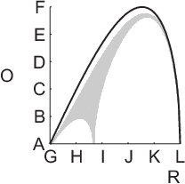
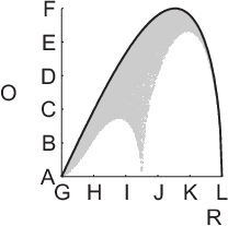
Figure 2 illustrates the result of Lemma 4. When (even), the lower bound is attained at every value of , which shows that the given bound is the tightest possible. However, as illustrated in the left panel, when , the bound is never attained except on the set . It can be shown however that in the limit of large the given bound is arbitrarily tight, even for odd , in the sense that for every ,
tends to zero as tends to infinity.
Lemma 4 has some interesting implications. For instance, it can provide insight into the rate at which solutions of a homogeneous system of Kuramoto oscillators ((2) with for ) on converge to fixed points, . To see this, consider the homogeneous system
| (40) |
where . We shall compute the time derivative of the magnitude squared of the order parameter, , and show that this derivative is: nonnegative along solutions of (40); () bounded from above by a certain function for every . We proceed as follows [9]. By definition,
Using the identity
it follows that
| (41) |
which shows that the time-derivative is positive everywhere, except at the equilibria, where it is zero. It follows that the magnitude of the order parameter is a nondecreasing function of time. Based on the observation that the time-derivative of is positive almost everywhere (the set of equilibria having measure zero), we formulate the following conjecture, [3, 9]:
Conjecture 1
For almost all initial conditions , the solution to the homogeneous system (40) has the property that .
In agreement with Conjecture 1, one can prove that, for the homogeneous system, the global phase-locking manifold is (locally) asymptotically stable. However, the existence of other invariant manifolds, not contained in , implies that is not globally asymptotically stable. We conjecture that is ‘almost globally asymptotically stable’, in the sense that its region of attraction is the entire space minus a set of measure zero.
For our next result, we shall need the concept of a dominating function, which is defined as follows:
Definition 3
Let and let be some interval. We say that dominates on if for all . In that case we call a dominating function for on .
Our next result states that is dominated by a certain scalar function that depends only on . In order to prove this result, we need the following two lemmas.
Lemma 5
Let be a solution of the homogeneous system (40) and suppose for some . Then
Proof: Recall that . It follows from the proof of Lemma 4 that for some if and only if one or two of the following conditions hold: (a) ; (b) is even and there exists a permutation of such that
| (42) | |||||
| (43) |
If , we have that for all and the result follows trivially. Now suppose Conditions (42) and (43) hold. It follows that for and , and hence
In other words, if satisfies Conditions (42) and (43) for some , it satisfies (42) and (43) for all . This concludes the proof.
Lemma 6
Let be such that for every , the systems
have unique solutions in . Let these solution be denoted and , respectively. Suppose there exists , , such that
for all . Then for every , we have that
| (44) |
for all , where is defined as
| (45) |
Proof: Under the hypotheses of the lemma we have that , and it follows that for small enough , (omitting the argument for notational convenience). Note also that and are increasing whenever and respectively. Now suppose there exists such that and . Then by continuity there exists such that and . Define . It follows that , which contradicts our starting hypothesis. We conclude that for all .
We have the following result:
Corollary 1
Let be a solution to the homogeneous system (40) with initial condition . Then
| (46) |
is a dominating function for on .
Proof: By Lemma 4 we have that for all . We claim that, on , is dominated by the solution of the ODE
| (47) |
which is given as
| (48) |
To prove this, suppose for some and let denote the smallest such (in case for all , the result follows immediately from Lemma 6). Then by Lemma 5, we have that for all , and it follows that
| (49) |
One can easily verify that is nondecreasing as a function of for all (and . Now let be an upper bound for . It follows that is a dominating function for on the interval . To compute an upper bound for , we proceed as follows. By definition of , we have that for all . It follows from Lemma 6 that
| (50) |
By continuity, we have that
Using the upper bound for , it follows from (49) that
| (51) |
Combining (50) and (51), we arrive at the desired result. This concludes the proof.
Figure 3 shows the graph of and that of the dominating function —Eqn. (46) for a particular realization of the initial condition . In this example, and . We observe that, in agreement with Conjecture 1, the solution converges to a globally phase-locked state, that is . Note that convergence can be very slow depending on the choice of initial condition. Indeed, for any and any , we can find such that if then for all . The upshot of this is that if the initial condition is selected by drawing from a uniform distribution and the number of oscillators is large, then is likely to be small, and as a consequence convergence to the stable equilibrium is likely to be slow. In the limit case when tends to infinity, we have that tends to zero with probability and the time required for to exceed some given finite threshold diverges to infinity.

Let denote the (sample) standard deviation associated with the vector of intrinsic frequencies . Using Lemma 4 we derive another lower bound on the critical coupling, as follows:
Corollary 2
The critical coupling satisfies
| (52) |
Proof: Let be a fixed point of the system (17). Then by definition and by Lemma 4 we have that
| (53) |
It is not hard to see that the right hand side of (53) is upper bounded by . It follows that
| (54) |
This completes the proof.
Note that Corollary 2 is in agreement with the intuition that greater variation in intrinsic frequencies requires stronger coupling to achieve global phase-locking.
Using Lemma 4 we can compute bounds on the value of the order parameter evaluated at the fixed points of the system, should they exist. Indeed, suppose , then for any fixed point we have that
| (55) |
Solving for gives
| (56) |
The graph associated with inequality (56) is shown in Figure 4.

5 Necessary and Sufficient conditions
In the last section, we derived lower bounds for the critical coupling of the system (17), which provide necessary conditions for the existence of fixed points. We next derive conditions that are both necessary and sufficient for fixed points to exist, and we shall use these results to describe an algorithm for computing the critical coupling in Section 6.
Throughout this section, the function is given by (2.2) and the set is defined as
On we introduce a notion of equivalence, as follows.
Definition 4 (Equivalence on )
Given and , let . We say that and are equivalent () if .
To motivate this definition consider the following fact. Let be given, and let be such that . If is a fixed point of the system (17), then is also a fixed point of the system (17) and, in addition, .
The following theorem provides a necessary and sufficient condition for the system (17) to have a fixed point, given a particular coupling strength , and a particular realization of intrinsic frequencies, .
Theorem 2
Let and . Then iff there exists and such that
| (57) |
Moreover, suppose and both satisfy (57) and let be such that
| (58) |
Then iff and .
Proof: Suppose (the case is easy). Let be a fixed point of (17). By definition, , and since , we have that , and consequently . It follows that
| (59) |
Let . By (59) we have that . Recall that for all , can be written as
| (60) |
and let be given as
| (61) |
Combining (59), (60), and (61), we arrive at
| (62) |
This proves necessity. To prove sufficiency, let be given, and suppose (again, the case is easy). Then for every , the system
| (63) |
has a unique solution . We pick such that . Since , it follows that
| (64) |
From (63), we have that
| (65) |
Combining (64) and (65), we arrive at
| (66) |
The second part of the theorem follows easily after noting that if satisfies (58) then , .
Theorem 2 gives us a necessary and sufficient condition for the equation to have at least one solution for a given value of . It is not clear, however, that there exists a for which this condition is satisfied. The following Corollary provides an easy sufficient condition.
Corollary 3
Let and . Suppose
| (67) |
for some . Then .
Proof: Suppose (again, the case is easy). Let . Define , and ,
| (68) |
Since we have that . Now suppose condition (67) is satisfied. Then we have that , and by the Intermediate Value Theorem there must exist such that . It follows from Theorem 2 that the system (17) has a fixed point.
Corollary 4
Let . Then: the critical coupling is finite; for large enough coupling, the system (17) has at least fixed points.
Proof: Note that the right hand side of (67) does not depend on . Hence, it follows that, provided
| (69) |
Condition (67) is always satisfied for large enough . Furthermore, it follows easily that if (69) is not satisfied for given , then it is satisfied for . This implies () that the critical coupling is always finite, and () that the set contains precisely elements (counting multiplicity), each of which defines a unique (up to equivalence in the sense of Definition 4) fixed point. This concludes the proof.
Corollary 5
Let and . Then if and only if there exist such that
Proof: The proof of Corollary 3 suggests that if the fixed point equation (57) does not have a solution, then necessarily
for all and for all . Since we have that
for all , it follows that the given condition is necessary and sufficient for the system (17) to have at least one fixed point. This concludes the proof.
The next and final corollary gives us an upper bound on the critical coupling.
Corollary 6
The critical coupling, , satisfies:
| (70) |
Proof: Follows directly from Corollary 3.
6 An algorithm for computing
In this section we present a bisection algorithm that will allow us to numerically evaluate the critical coupling with arbitrary precision. Throughout, we shall assume that . Define , and let , and be given as
| (71) |
Also, define ,
| (72) |
From Corollary 5 it follows that the critical coupling is the smallest for which the equation has at least one solution on . We have the following result.
Theorem 3
For all , , the equation
| (73) |
has a unique solution , and we have that
| (74) |
Proof: Observe that, by strict concavity of and linearity of , the equation can have at most two solutions on for any . We shall now show that, when , it can have no more than one solution. Since, by definition of critical coupling, must have at least one solution, we shall conclude that it has precisely one solution. Let and suppose there exist , , such that and . By strict concavity of we have that . Define and note that . We have that . This implies that there exists such that . But by definition is the smallest for which has a solution. We arrive at a contradiction and conclude that ; or in other words, that the equation has exactly one solution on . Denoting this solution by , it is not hard to see that, at , the derivative of with respect to and the derivative of with respect to (both of which are defined on the entire interval ) must coincide. For suppose , then by continuity there exists such that for all such that . Let be one such . It follows that there exists such that . This leads to a contradiction and we conclude that . By analogy we have that . We conclude that . That is,
| (75) |
Or equivalently,
| (76) | |||||
Now recall that by definition of , we have that
| (77) |
Equating the right hand side of Eqn. (76) with the right hand side of Eqn. (77) gives
| (78) |
This shows that is a solution to (73). What remains to be shown is that is the only solution. Define ,
and note that, on their respective domains, is strictly monotonically decreasing while is strictly monotonically increasing. In addition, note that there exist such that and . Hence, by continuity, there must exist a point such that . Monotonicity of and implies that this point is unique. It follows that is the unique solution of (73) on . And by (77) we have that
| (79) |
This concludes the proof.
Based on the result of Theorem 3, we define the map ,
| (80) |
where, as before, denotes the unique solution of (73) on , given . Note that, given any realization of such that , we have that . We have the following corollary.
Corollary 7
- 1.
For all , , we have that ;
- 2.
there exists such that if and only if is even;
- 3.
for every there exist an positive integer and such that .
Proof: (Part 1). We show that for all , the solution of equation (73) satisfies . The result then follows easily. Let . Then we have that
It follows that
for all . The lower bound
was obtained earlier in
Section 4.
(Part 2.) From the above it follows that if and only if
or equivalently, for all . It is easy to see that this latter condition is never satisfied when is odd (keeping in mind that ). Now suppose is even and pick any . Define
Then we have that . Moreover, for all . It follows that .
(Part 3.) Let be given and suppose is odd. Pick and define
Then (73) evaluates to
| (81) |
and it is not hard to see that as tends to infinity, the solution of (81) tends to . Indeed, for we have
| (82) |
Let , and pick such that and . It follows that
| (83) |
and hence
| (84) |
Now let be given as and choose accordingly. It follows that . This concludes the proof.
We are now ready to present our algorithm, which, given , will compute with user-defined precision in a finite number of iterations, .
Algorithm 1
- 1.
,
- 2.
While ,
- 3.
.
- 4.
If then , else .
- 5.
End.
Once we have an estimate of , we can use (74), replacing with , to estimate .
7 Numerical Example
We illustrate the results presented in this paper by means of a numerical example. We consider two systems with and oscillators respectively, with frequencies as depicted in Figure 5.
 |
 |
| (a) | (b) |
The frequencies in this example were sampled from a normal distribution with zero mean and unit variance and relabelled such that (note that this can be done without loss of generality). For this particular realization of (), we have that ( and
It follows from Corollary 6 that () and by (32), we have that (). Figure 7 shows the time evolution of the magnitude squared of the order parameter, (previously denoted as ), for two different initial conditions and two values of the coupling coefficient, and ( and ). We observe that when is slightly greater than the known lower bound on , the value of converges to a constant and inspection shows that the solution of the system (17) tends to a fixed point. On the other hand, when the coupling coefficient is slightly below the known upper bound on the critical coupling, the trajectories appear not to converge. Note that in this case we do not know whether the system (17) has a fixed point or not, as the condition stated in Corollary 6 is only sufficient while at the same time the respective coupling strengths exceed their known lower bounds ( and respectively). To gain more insight into this situation let us consider the case in some more detail. We fix the coupling coefficient at , and numerically evaluate the function ,
| (85) |
for several values of in the interval . We repeat the same computation for . The result is shown in Figure 8. We observe that the equation does not have a solution on the interval when , but does have a solution when .
We use Algorithm 1 to compute the ‘exact’ value of the critical coupling to the fifth significant digit. We find that for the case and for the case . Note that in both cases, but particularly the latter, the upper bounds ( and respectively) provide good estimates of the true values of the critical coupling.
 |
 |
| (a) | (b) |
 |
 |
| (a) | (b) |


8 Conclusion
We derived necessary and sufficient conditions for the existence of fixed points in a finite system of coupled oscillators. In particular, we derived an easy sufficient condition in terms of the individual oscillator frequencies (Corollary 3), which we used to compute an upper bound on the critical coupling (Corollary 6). We showed that when no prior knowledge of the distribution of frequencies is available, we can still bound the critical coupling in terms of the infinity norm of the frequencies with their mean removed (Corollary 7). These bounds were shown to be the tightest possible, in the sense that we can find realizations of the intrinsic frequencies for which the upper bound is attained, and others for which the critical coupling is arbitrarily close to the lower bound. Finally, we proposed an efficient algorithm (Algorithm 1) for computing the critical coupling to within arbitrary bounds in a finite number of steps. In future work we shall seek to extend the present analysis to complex networks of arbitrary topology, and investigate more closely the impact of the shape of the distribution of intrinsic frequencies on the value of the critical coupling. We shall also consider the important question of stability, and present analytical results for the limit case when the number of oscillators tends to infinity.
References
- [1] J. Acebrón, L. Bonilla, C. Pérez Vicente, F. Ritort, and R. Spigler. The kuramoto model: a simple paradigm for synchronization phenomena. Reviews of Modern Physics, 77:137–185, 2005.
- [2] A. Beuter, L. Glass, M.C. Mackey, and M.S. Titcombe, editors. Nonlinear Dynamics in Physiology and Medicine. Springer, 2003.
- [3] N. Chopra and M. Spong. On synchronization of kuramoto oscillators. In Proceedings of the 44th IEEE Conference on Decision and Control, Seville, Spain, pages 3916–3922, 2005.
- [4] R. Diestel. Graph Theory. Springer-Verlag, 2000.
- [5] L. Glass. Synchronization and rhythmic processes in physiology. Nature Review, 410:277–284, 2001.
- [6] M. Golubitsky and Ian Stewart. Nonlinear Dynamics of Networks: the Groupoid Formalism. Bulletin of the American Mathematical Society, 43(3):305–364, 2006.
- [7] H. Hong, M. Choi, and B. Kim. Synchronization on small-world networks. Physical Review E, 65(026139), 2002.
- [8] H. Hong, H. Park, and M. Choi. Collective synchronization in spatially extended systems of coupled oscillators with random frequencies. Physical Review E, 72(036217), 2005.
- [9] A. Jadbabaie, N. Motee, and M. Barahona. On the stability of the kuramoto model of coupled nonlinear oscillators. In Proceedings of the American Control Conference, Boston, USA, pages 4296 – 4301, 2004.
- [10] Y. Kuramoto. Self-entrainment of a population of coupled nonlinear oscillators. In H. Araki, editor, International Symposium on Mathematical Problems in Theoretical Physics, volume 39 of Lecture Notes in Physics. Springer, 1975.
- [11] Y. Kuramoto. Chemical Oscillations, Waves and Turbulence. Springer, 1984.
- [12] Y. Maistrenko, O. Popovych, and P. Tass. Desynchronization and Chaos in the Kuramoto Model, volume 671 of Lecture Notes in Physics. 2005.
- [13] Y. Maistrenko, V. Popovych, O. Burylko, and P. Tass. Mechanism of Desynchronization in the Finite-Dimensional Kuramoto Model. Physical Review Letters, 93(8), 2004.
- [14] Y. Maistrenko, V. Popovych, and P. Tass. Chaotic Attractor in the Kuramoto Model. International Journal of Bifurcation and Chaos, 15(11):3457–3466, 2005.
- [15] Y. Moreno and A. Pacheco. Synchronization of kuramoto oscillators in scale-free networks. Europhysics Letters, 68:603–609, 2004.
- [16] J.D. Murray. Mathematical Biology. Springer, 3rd edition, 2002.
- [17] A. Pikovsky, M. Rosenblum, and J. Kurths. Synchronization: a universal concept in nonlinear sciences. Cambridge University Press, 2003.
- [18] V. Popovych, Y. Maistrenko, and P. Tass. Phase chaos in coupled oscillators. Physical Review E, 71(065201), 2005.
- [19] J. Rogge and D. Aeyels. Existence of partial entrainment and stability of phase locking behavior of coupled oscillators. Progress of Theoretical Physics, 112:921–942, 2004.
- [20] J. Rogge and D. Aeyels. Stability of phase locking in a ring of unidirectionally coupled oscillators. Journal of Physics A, 37:11135–11148, 2004.
- [21] R. Sepulchre. Oscillators as systems and synchrony as a design principle. In L. Menini, L. Zaccarian, and C. T. Abdallah, editors, Current trends in nonlinear systems and control, Lecture Notes in Control and Information Sciences. Birkhauser, 2006.
- [22] R. Sepulchre, D. Paley, and N.E. Leonard. Group coordination and cooperative control of steered particles in the plane. In K. Y. Pettersen, J. T. Gravdahl, and H. Nijmeijer, editors, Group Coordination and Cooperative control, Lecture Notes in Control and Information Sciences, pages 217–232. Spinger-Verlag, London, 2006.
- [23] S. Strogatz. From kuramoto to crawford: exploring the onset of synchronization in populations of coupled oscillators. Physica D, 143:1–20, 2000.
- [24] S. Strogatz. Exploring complex networks. Nature, 410:268 – 276, 2001.
- [25] M. Verwoerd. Fixed-point analysis of a finite system of kuramoto oscillators. In Proceedings of the Fourth Irish Conference on the Mathematical Foundations of Computer Science and Information Technology (MFCSIT), Cork, Ireland, 2006.
- [26] M. Verwoerd and O. Mason. Conditions for the existence of fixed points in a finite system of kuramoto oscillators. In Proceedings of the American Control Conference, New York, NY, pages –, 2007.
- [27] D. Watts and S. Strogatz. Collective dynamics of ’small-world’ networks. Nature, 393(6684)(6684):440–2, 1998.