Diffractive Excitation in DIS and CollisionsPreprint: LU-TP 07-25
Abstract:
We have in earlier papers presented an extension of Mueller’s dipole cascade model, which includes subleading effects from energy conservation and running coupling as well as colour suppressed effects from pomeron loops via a “dipole swing”. The model was applied to describe the total cross sections in and collisions.
In this paper we present a number of improvements of the model, in particular related to the confinement mechanism. A consistent treatment of dipole evolution and dipole–dipole interactions is achieved by replacing the infinite range Coulomb potential by a screened potential, which further improves the frame-independence of the model.
We then apply the model to elastic scattering and diffractive excitation, where we specifically study the effects of different sources for fluctuations. In our formalism we can take into account contributions from all different sources, from the dipole cascade evolution, the dipole–dipole scattering, from the impact-parameter dependence, and from the initial photon and proton wavefunctions. Good agreement is obtained with data from the Tevatron and from HERA, and we also present some predictions for the LHC.
Keywords:
Small- physics, Saturation, Diffraction, Dipole Model, DIS1 Introduction
In high energy scattering the cross section for parton–parton subcollisions becomes larger than the total cross section. This means that on average there are more than one subcollision in a single event, and it was early suggested that hard subcollisions dominate the features of high energy scattering and are the cause of the rising cross section. This is also the basic assumption in the model by Sjöstrand and van Zijl [1] implemented in the P YTHIA event generator, which is able to describe many features of high energy collisions.
That perturbative dynamics dominate high energy collisions is also supported by the large intercept of the BFKL pomeron. Via unitarity and the AGK cutting rules, the large subcollision cross section and high probability for multiple collisions have also strong implications for diffraction. Hard diffraction was first observed by the UA8 collaboration at the CERN Spp̄S collider [2], and has later been studied in much more detail both at the Tevatron (see e.g. [3, 4]) and at HERA (see e.g. [5, 6]).
Multiple collisions, unitarity and saturation are conveniently studied in terms of dipoles in transverse coordinate space. The dipole model by Golec-Biernat and Wüsthoff (GBW) [7, 8] has successfully described both and diffraction in DIS. Mueller’s dipole cascade model [9, 10, 11] reproduces the leading log (linear) BFKL equation, and includes also multiple collisions and satisfies the unitarity constraint. The multiple collisions correspond to pomeron loops. Mueller’s model includes, however, only such loops which are cut in the particular Lorentz frame used in the calculation, but not loops which are fully contained in one of the individual dipole cascades. Many attempts (see for example [12, 13] and references therein) have been presented including e.g. , or more complicated dipole vertices, but so far no explicitly frame-independent formalism has been presented.
As discussed in some detail below, an important part of the NLL corrections to the BFKL equation are related to energy conservation. In a series of papers [14, 15] we have developed Mueller’s model to include both effects of energy–momentum conservation and effects of pomeron loops and saturation inside the cascade evolution via a dipole transition, called a dipole swing. The swing does not reduce the number of dipoles, rather the saturation effect is achieved as the ”new” dipoles are smaller, and therefore have smaller cross sections. Although not explicitly frame independent, the numerical result is almost independent of the frame used for the calculations. With a simple model for the proton in terms of three dipoles, the Monte Carlo implementation also reproduces the total cross section both for DIS at HERA and for scattering from ISR energies to the Tevatron.
In this paper we will first make some technical improvements related to confinement, and then use the model to study diffractive scattering at HERA and the Tevatron. The perturbative calculation has some problems in the IR region, especially with a running coupling, and a cutoff for large dipoles is essential for the frame independence and the good agreement with data. We here propose to treat this effect of confinement by everywhere replacing the Coulomb colour-electric potential by a screened Yukawa potential.
Both the screening length and the size of the initial proton wave function are determined by the confinement mechanism. In the MC implementation these two quantities are assumed to be of the same size. This implies that for -collisions and DIS at high the model has only two tunable parameters; besides only the confinement scale denoted by . For smaller the result is, however, also sensitive to the quark masses in the virtual photon wave function. The value of turns out to be very important in order to obtain the correct normalization for in collisions, but the increase of with the center of mass energy is found to be much less sensitive to this parameter. Once is fixed to obtain the correct normalization for in scattering, the DIS cross section is obtained without any further changes.
Our treatment of elastic scattering and diffractive excitation is based on the eikonal approximation and the Good and Walker picture [16]. The result is determined by the fluctuations in the collision process originating from the initial wave functions of the proton and the virtual photon, from the dipole cascades and from the dipole–dipole scattering probability. In our formalism all these different components give important contributions. One result of this is that the impact parameter profile is less steeply falling, i.e. less black and white and more “grey”, than in models where the dominant fluctuations are assumed to come from fluctuations in the impact parameter, .
The distribution in the mass, , of the diffractive state can be obtained by a study of the collision in different Lorentz frames, as discussed by Hatta et al. [17]. (It is here essential that we have a frame-independent formalism.) However, in addition to the fluctuations included in this reference and in the GBW approach, we also include fluctuations in the evolution of the proton target.
In section 2 we review briefly the dipole cascade model, discuss the modification of the confinement effect, and demonstrate the frame independence of the model. In section 3 we discuss the formalism for elastic and diffractive scattering, and the effects of the different sources of fluctuations in the collision process. Our results are presented in section 4, and the conclusions in section 5.
2 Dipole Model and Frame Independence
We will in this section briefly discuss the cascade model presented in refs. [14, 15], describe the modified treatment of confinement, and demonstrate the frame independence by showing some quantitative examples.
2.1 Mueller’s cascade model
The model is based on Mueller’s dipole formalism [9, 10, 11] in which the small- evolution is interpreted in terms of a dipole cascade. The probability per unit rapidity that a dipole emits a gluon at transverse position is here given by
| (1) |
and the evolution of the cascade agrees with the leading order BFKL evolution. As a consequence, the total number of dipoles grows exponentially. This also implies a strong growth for the total cross section which, however, is tamed by taking multiple dipole interactions into account. The scattering probability between two elementary colour dipoles with coordinates and respectively, is given by
| (2) |
Since Mueller’s model is formulated in transverse coordinate space, multiple scatterings can be included in an eikonal approximation, and a unitarised expression for the total scattering amplitude can be obtained as
| (3) |
2.2 Energy conservation
The fast growth in leading order BFKL is much reduced by NLL effects. As discussed in ref. [18], besides effects from the running coupling (which are also included in our simulations) the NLL corrections to BFKL evolution are related to the non-singular terms in the splitting function, and to the so called energy scale terms, and both these effects are related to the conservation of energy and momentum. It should be noted, however, that although these NLL corrections to the evolution kernel are essential for the conservation of energy and momentum, they are not sufficient to guarantee global energy-momentum conservation, which is most easily achieved in a computer simulation [19].
The LL BFKL result is obtained from the singular term in the gluon splitting function, which dominates for small . The recoil for the gluon taking the fraction is here neglected. However, for large -values energy conservation implies that this recoil cannot be neglected. (More precisely it is conservation of the positive light-cone component, as in a boost invariant formalism the variables and are defined as fractions of .) If this suppression can be described by an effective cutoff (with ), an integral over is replaced as [20]
| (4) |
As discussed in ref. [21] the effect of the non-singular terms in the splitting function is just such a suppression of large -values, with .
The so called energy scale terms are needed in order for a non--ordered ladder to look the same if evolved from the bottom up or from the top down. Thus a step down in must look exactly like a step up in , if generated in the opposite direction. This implies that the cascade must be ordered not only in (via the constraint ) but also in the negative light-cone momentum . This constraint is therefore also related to energy-momentum conservation, and it corresponds to what is commonly called the consistency constraint. As discussed in refs. [20, 22], it has the consequence that the pole in the characteristic function is replaced by . The minimum of is then shifted to , and thus a distance further away from the poles. Expanding this effect to lowest order in gives the energy scale terms presented in ref. [18].
Using the similarities between Mueller’s cascade model and the Linked Dipole Chain (LDC) model [20, 22], we implemented energy–momentum conservation in the dipole cascade in ref. [14]. The of the partons was here associated with the dipole sizes in coordinate space. Although the number of dipoles still increases exponentially, the growth is significantly reduced and the onset of saturation is delayed.
2.3 Initial proton and photon wave functions
2.3.1 Photon
The splitting can be calculated perturbatively, and we use the well known leading order results for longitudinally and transversely polarized photons:
| (5) | |||||
Here is the negative light-cone momentum fraction of the photon carried by , and is the transverse separation between and , and we consider four active quark flavours, with an effective light quark mass of 60 MeV and a charm mass of 1.4 GeV, as described in [23].
Although the wave functions in eq. (5) are well known, there are still ambiguities in the initial phase of the evolution of the dipole cascade. This problem is an unavoidable consequence of the difficulty to reconcile the fundamentally quantum mechanical process with the semiclassical approximation represented by the cascade evolution.
For a given in DIS, the total rapidity range available for final state particles is given by , where is of the order of11 1 In the following the scale GeV will be omitted in writing logarithms. 1 GeV. We use a Lorentz frame such that an interval is on the photon side and the remaining interval is on the proton side. The kinematics is illustrated in figure 1, which shows the phase-space diagram for a DIS event in the -plane. Here the positions of the and are also indicated. Their distance in rapidity from the photon end are given by and respectively, where is the transverse momentum of the quark and the antiquark.
In the simulations we have assumed that gluon emission is possible only at rapidities larger than the rapidity of both and . We also identify with its typical value . As can be seen from figure 1, this implies that the interval allowed for the photon-initiated cascade is given by
| (6) |
Thus depends on both variables and . The total range for the evolution
| (7) |
may be larger or smaller than . One could also imagine other choices, but we want to emphasize that the difference is subleading in , and therefore the optimal choice cannot be determined from QCD with present techniques.

Anticipating the discussion in the following sections, we want in connection to figure 1 mention that a calculation of the diffractive cross section corresponds to events which have a gap at in this particular Lorentz frame. This means that the diffractively excited photon is confined within the rapidity range corresponding to a mass limited by .
2.3.2 Proton
The initial proton wavefunction can obviously not be determined by perturbation theory, but has to be specified by a model. Our assumption is that the initial proton can be described by three dipoles in a triangular configuration, where the corners could be associated with the three valence quarks. We admit that this model has deficiencies, and it should not be used to study the particle distribution in the proton fragmentation regions. The corner connecting two dipoles in a triangle corresponds to an octet colour charge, and not a quark triplet, and an alternative model could be three dipoles connected by a junction in a Y-shaped configuration. This would imply the need for extra assumptions about the behaviour of the colour-neutral junction, and we also believe that the enhanced radiation from the three colour octets might mimic radiation from gluon contributions present in the proton structure also at low virtuality.
We have tried two different triangular shapes. In the first one the triangle is assumed to be equilateral. In this case the size of the dipoles is assumed to be distributed according to a Gaussian
| (8) |
We found in ref. [15] that this simple model gives a very good agreement with data on cross sections for both scattering and DIS. To test the sensitivity to this simple assumption, we have now also studied a model where the triangle is not equilateral, but has an arbitrary shape. Also here the distribution is given by a Gaussian in the sizes of the three sides, , and ,
| (9) |
The results of the two models are very similar, and we will therefore in the following mainly present results obtained with the simple model given by .
The parameter , which determines the initial dipole size in the proton, is here assumed to be the same as the confinement scale in the cascade evolution and the dipole–dipole scattering (see section 2.5 below). Along with , it is one of the essentially two free parameters of our model. We note, however, that the variation of these two parameters have similar effects. Thus an increased value for can be compensated by a reduced value for (and vice versa), leaving the cross sections unchanged as seen in figure 2. We note in particular that the energy dependence is rather insensitive to the parameters chosen.
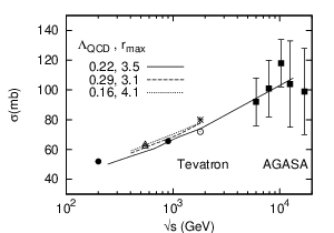
The probability for a three-body system to contract to a single point should be zero, and we have therefore also tested a wavefunction where small -values are suppressed but where has the same value. We then find essentially the same results for total cross sections, but the reduced fluctuations imply that the cross sections for elastic scattering and single diffractive excitation become larger. This feature will be further discussed in sections 3.2.2 and 4.
2.4 Dipole swing
One problem with Mueller’s model is the fact that saturation effects are not included inside the individual dipole cascades. Thus only pomeron loops which are cut in the particular Lorentz frame used are taken into account, and the result is not frame independent. Non-linearities due to multiple interactions are included, but the evolution of the dipole cascades obey the linear BFKL equation.
We argued in ref. [15] that the missing saturation effects can be taken into account by including the so called dipole swing in the evolution. Although there is no analytical proof that this would give a frame independent formalism, numerical simulations in a MC implementation showed that the resulting evolution is approximately frame independent. We will show this in more detail in subsection 2.6.
The swing is a process in which two dipoles and are replaced by two new dipoles and . The process can be interpreted in two ways. The quark at and the antiquark at form a colour singlet with probability . In this case the best approximation of the quadrupole field ought to be obtained by the closest charge–anti-charge combinations. Here the swing is therefore naturally suppressed by , and it should be more likely to replace two given dipoles with two smaller ones. Secondly, we may see it as the result of a gluon exchange between the dipoles, which results in a change in the colour flow. In this case the swing would be proportional to , which again is formally suppressed by , compared to the splitting process in eq. (1), which is proportional to .
In the MC implementation each dipole is randomly given one of possible colour indices. Only dipoles with the same colour index can swing, and the weight for a swing is determined by factor proportional to
| (10) |
This implies that the swing favours the formation of smaller dipoles. The number of dipoles is not reduced by the swing, but the fact that smaller dipoles have smaller cross sections gives the desired suppression of the total cross section.
The swing is instantaneous in for both the colour multipole and gluon exchange interpretations. It is therefore not a vertex in the sense of the dipole splitting whose probability is proportional to . In the MC implementation the swing is formulated as if it was proportional to , but its strength is adjusted so that it is effectively instantaneous. In ref. [24] it is shown that combining the dipole splitting and the dipole swing, one can reproduce all colour correlations induced from the multiple dipole interactions. In case each dipole is restricted to single scattering, one can combine a splitting with one swing at a time to reproduce all correlations, but without this restriction, the maximum number of simultaneous swings needed in combination with a splitting, for a system consisting of dipoles, is .
2.5 Consistent treatment of confinement
As the dipole model is formulated within perturbative QCD, confinement effects are naturally not included. Obviously, one cannot let the dipoles in the cascade become too large, and it is then natural to introduce a scale, such as our parameter, so that large dipoles are suppressed.
Similarly, the scattering of dipoles is calculated perturbatively, and the interaction range is therefore longer than what we would expect from confinement. The formula for in eq. (2) is just the two dimensional Coulomb potential which for large distances behaves as
| (11) |
where is the impact parameter of the dipole–dipole collision. Thus the scattering probability falls off only as a power of , and not as an exponential as one would expect from a confining field. The expression for can be written as
| (12) |
where is the Green’s function given by
| (13) |
To take confinement into account we can replace the infinite range Coulomb potential with a screened Yukawa potential. This implies that the Coulomb propagator in eq. (13) is replaced by , where is the confinement scale. In this case the integral in eq. (13) is replaced by
| (14) |
where is a modified Bessel function. The expression in eq. (2) is then replaced by
| (15) |
For small separations where , the function behaves like ln and we then immediately get the result in eq. (2). For large separations where , falls off exponentially , as expected from confinement.
To be consistent we should then also modify the dipole splitting kernel accordingly. The dipole splitting probability in eq. (1) can be written in the form
| (16) |
The two terms in this expression are each obtained from the integration
| (17) |
Once again making the change , and noting that , we may replace eq. (16) by
| (18) |
For small arguments , from which we get back the result in eq. (16), while for large arguments , and once again we obtain an exponentially decaying field.
2.6 Frame independence
We will in this subsection demonstrate the frame independence by showing some explicit results obtained using the MC implementation.
The cross section obtained when the right-moving (left-moving) cascade is evolved a rapidity distance () is denoted , and in figure 3 we show the relative difference plotted vs. . The figure shows results both including the dipole swing and without the swing. Without the swing the cross section is too large when or . As expected, the degree of frame dependence is increasing for larger , when the saturation effects within cascades become more important. When we include the swing, we see that the cross section is (within errors) independent of the Lorentz frame used.


Figure 4 shows similar results for DIS. Here the cross section is not exactly frame independent, with a tendency of getting larger as we give more of the total rapidity interval to the evolution of the photon. (This may not be very clear from the figures shown but it can be seen more clearly for dipole-proton scattering where we do not have ambiguities in choosing the interval as in DIS.) There seems to be two causes for this behaviour, and neither of them are related to saturation or the dipole swing. The first cause is the running of the coupling, especially when the dipole–dipole scattering amplitudes are calculated (see next subsection). The second cause is the treatment of energy conservation in the dipole–dipole scattering. In case we use a fixed coupling when calculating the scattering amplitude (but still using a running coupling in the evolution), the result appears to be more frame independent. These issues need to be handled more carefully, and we intend to look at them in forthcoming publications. Note however that the difference is less than 10 percent for both values, and it is also not dependent on the energy. As our model is not expected to have a better accuracy than this, we can consider the model to be essentially frame independent also for DIS.
2.7 Running Coupling
In our simulations we use a running both in the dipole splitting and in the dipole–dipole scattering probability. Recent NLO studies of the dipole evolution [25, 26] have revealed a fairly complicated structure for the running of . However, in [27] this was shown to simplify in the strongly ordered limits, implying that the relevant scale in the dipole splitting is determined by , where is the mother dipole which splits into and . This is also the scale we have been using in our simulations.
For the dipole–dipole scattering, the situation is more complicated. We have two powers of and there are six different scales involved. With the two colliding dipoles and we have besides, their sizes, also the distances , , and (cf. eq. (12)). Here we have tried two alternatives. In the first case the scale of for both powers is determined by . In the second case, we associate one to each of the colliding dipoles and choose the scales and respectively. To avoid divergencies, is frozen below the scale .
It turns out that the degree of frame dependence in is similar in both cases and the results presented in this paper have all been calculated using the first alternative.
3 Diffractive and elastic scattering in the dipole model
3.1 Formalism
In this section we will describe the formulas we are going to use in calculating the various diffractive and elastic cross sections. We shall rely on the dipole version of the Good and Walker picture of diffraction [16] where the scattering eigenstates are given by the dipole states. The identification of the QCD parton states as the eigenstates of diffraction is due to the work of Miettinen and Pumplin [28]. The situation is complicated by the fact that the states of the proton or the virtual photon depend on the Lorentz frame used, and we will here quite closely follow the formalism presented in [17].
In the Good and Walker picture of diffraction there is a normalized and complete set of real particle states with fixed quantum numbers. In addition we have eigenstates of the scattering, , which also form a complete set of normalized states. Assume that we have two incoming particles, one right-moving particle and one left-moving particle . These particles can then be diffracted onto the various particle states and , which carry the quantum numbers of and respectively. The incoming wave is given by
| (19) |
The scattered wave is obtained by operating with Im on , where is the scattering operator. It reads
| (20) |
The probability for diffractive scattering is given by
| (21) |
We have here identified for both and with the probability distribution for the dipole configurations inside the particles. Note that the sum actually involves a sum over the dipole occupation number as well as integrations over the transverse coordinates of each dipole, together with sums over their colour and spin configurations.
Using the completeness of the states , the expression in eq. (21) can be written in the following form:
| (22) |
Here the first term on the RHS corresponds to elastic scattering, where both and emerge intact from the collision. The second (third) piece gives the probability of the excitation of () into one of the states () with () remaining intact. This corresponds to single diffractive excitation. Finally, the last term takes into account the fact that both and may transform into excited states and , which thus corresponds to double diffractive excitation.
We note that the different terms in eq. (22) correspond to different averages of . The sum of the single diffractive excitation and the elastic cross section can be calculated as follows
| (23) | |||||
where we used the completeness of the states ,
| (24) |
Each of the coefficients above is to be evaluated at a certain rapidity . The total rapidity interval between and is determined by the total cms energy of the process. For scattering is simply given by ln, while the situation is a bit more subtle in DIS. How we determine in DIS was discussed above in section 2.3.1.
In Mueller’s dipole model the scattering amplitude is given by the eikonal form , where is defined in eqs. (2), (3). The different contributions to the diffractive cross section in eq. (22) are then given by
| (25) | |||||
| (26) | |||||
| (27) | |||||
| (28) | |||||
Here () is the cross section for the diffractive excitation of (). Similarly and stand for the elastic and double diffractive cross sections respectively. Summing these four contributions we get the total diffractive cross section
| (29) |
Assume now that the state is evolved up to while is evolved up to , with the total rapidity interval. The total and elastic cross sections given by
| (30) |
are necessarily independent of due to the requirement of frame independence.
The diffractive cross section in eq. (29) is, however, not independent of . This expression gives the probability for diffraction at a particular value of , i.e. the chance that we find a rapidity gap around that particular . If we calculate e.g. at a specific , we obtain the cross section where the diffractively excited right-moving particle is confined within the rapidity range . This is approximately equivalent to a maximal diffractive mass given by . Taking the derivative with respect to therefore gives the mass distribution .
For the total diffractive cross section in eq. (29) we thus expect, in the case of the symmetric collision, a maximum when , and a decrease when either or . For asymmetric scattering as in DIS, we expect that it is easier to excite the photon. For a right-moving photon the diffractive cross section should therefore be smallest when . This discussion is in accordance with the analysis by Hatta et al. [17]. In this reference the diffractive excitation of the proton is neglected, while in our formalism we can also take the proton excitation into account.
The results obtained for pp collisions and DIS are presented in section 4.
3.2 Importance of fluctuations
The impact of fluctuations upon the small- evolution has gathered considerable interest lately. As mentioned above, the various expressions for the cross sections in formulas eqs. (25)-(28) are all obtained by taking different averages of the quantity . The diffractive excitation is therefore completely determined by the fluctuations in the colliding systems and the interaction probabilities.
3.2.1 Different sources
There are several sources of fluctuations in the various expressions in eqs. (25)-(28), related to variations in impact parameter, in the dipole cascades, and in initial the wave functions for the photons and protons. Many analyses include part of the fluctuations, assuming this to give the dominant contribution. Thus the dipole-saturation model by Golec-Biernat and Wüsthoff [7, 8] takes into account fluctuations in the photon wave function and the emission of the first gluon in the photon cascade, while the model of Kowalski and Teaney (KT) [29] emphasizes the fluctuations in the impact parameter. Hatta et al. [17] includes the fluctuations in the photon cascade, but assumes that the fluctuations in the proton cascade can be neglected. As a result fits to data can give different results for the impact parameter profile, and different approaches can give different ratios for the elastic cross section and diffractive excitation. As an illustration we will here compare the fluctuations in our model with those in the Kowalski–Teaney model.
In the KT model the differential dipole–proton cross section in impact parameter space is given by the eikonal
| (31) |
where is the dipole size. The opacity is modeled by a factorized form
| (32) |
where is the transverse profile function of the proton. In there is also a dependence on which is omitted here. To determine the impact parameter profile it is assumed that the dependence of the diffractive vector meson production cross section is given by an exponential, which in turn implies a Gaussian profile for . The two unknown parameters of this Gaussian are then determined by a fit to diffractive production data.
For a virtual photon the only fluctuations are those in the dipole size, , and impact parameter, . The diffractive cross section is calculated as
| (33) |
where .
When comparing the two models it may seem natural to compare with the average , where denotes the averaging over the dipole and proton cascades and the initial proton wavefunction. The corresponding total and diffractive cross sections would then read
| (34) | |||||
| (35) |
This is, however, not necessarily correct. The opacity is in the KT model determined by a fit to data for the total cross section. What is directly determined is therefore , rather than itself. Thus a more direct analogy to our model would be the quantity , which would give the same total cross section as eq. (30) and imply the following form for the diffractive cross section:
| (36) |
Note that this is not the same as the elastic contribution in eq. (25) since in that case also the photon wave function is included in the squared average (eq. (25) is meaningless in DIS since the virtual photon cannot scatter elastically).
The expressions in eq. (35) and eq. (36) should be compared with the results in our model, obtained by integrating eq. (29) over :
| (37) |
Such a comparison is interesting as a way to gauge the role played by the fluctuations.


The results obtained from eq. (35) and eq. (36) are shown in figure 7, together with the results obtained from eq. (37) which includes all fluctuations. We immediately notice the very large effects in our model from the fluctuations in the cascades and the proton wave function. The diffractive cross section calculated from eq. (35) is seen to be a factor 2-3 below the result obtained from eq. (37), while the result from eq. (36) is around a factor 4 lower than eq. (37).
We conclude that in our model a large fraction of the fluctuations determining the diffractive cross sections is caused by the dipole cascade evolutions. In order to obtain a similar result in the KT model it is therefore necessary to have larger fluctuations due to the impact parameter dependence, which means an impact parameter profile which is more narrow, i.e. more black and white compared to Mueller’s dipole cascade model, where the average scattering can be “grey” overall, since the fluctuations in the cascades means that some events are almost black while other are almost white. This can clearly be seen in figure 8 where we compare the impact parameter profile from the KT model to that obtained from our model. (A similar effect, although less pronounced, is observed in the profile for scattering presented in ref. [15]. Also here the profile obtained in our model has a somewhat higher tail for large impact parameters than the Gaussian fit to Tevatron data by Sapeta and Golec-Biernat [30].)

3.2.2 Wave functions
Photon
The photon wave functions in eq. (5) for longitudinal and transverse photons are fully determined by perturbation theory. We note that these wave functions are not normalized, even for real photons. This is, however, not in contradiction with the assumption that the states are normalized. The generic photon state can be written
| (38) |
where is the component of the photon coupling directly to the quarks. While the state is normalized, the two separate components above are not. Rescattering of the component can be neglected, as it is proportional to . It is therefore sufficient to only keep the contribution from , which is not a normalized state.
In DIS it is not meaningful to consider the elastic scattering, as the virtual photon can never be detected as a real particle. The closest analogies to elastic scattering are given by Deeply Virtual Compton Scattering (DVCS) and the exclusive reactions , with a vector meson. We will return to these processes in a future publication.
Proton
The wave function for the proton is much less well defined. The expressions in eqs. (8) or (9) ought to be interpreted as probability distributions rather than quantum mechanical wave functions, which can be used to determine the interference effects present in eqs. (25)-(28). The fluctuations in the wave functions influence the terms in eqs. (25)-(28) in which the average of is taken before the square (i.e. events containing an elastic proton).
As discussed in section 2.3.2 a wave function where three particles can simultaneously be in a single point is not realistic. A Gaussian distribution in impact parameter is usually motivated by the exponential dependence on for the elastic cross section. However, the constant -slope is (except possibly for the highest Tevatron energy) only valid for , corresponding to , and therefore a suppression for small is still compatible with this constraint. Simulations with such a wave function reduces the fluctuations and increases the cross sections for elastic scattering and single diffractive excitation, while leaving the total and the total diffractive cross sections unchanged, provided the average is kept the same.
There is, however, also a more fundamental problem with the proton wave function. In the Good and Walker formalism the hadronic states form a complete set. This implies that before the cascade has started, there must be other hadron states with wavefunctions orthogonal to the proton wavefunction. This calls for a detailed dynamical scheme describing the relevant degrees of freedom for the hadronic states. With the approximation these orthogonal states also have the same mass as the proton, which increases the problem further.
Lacking a real quantum-mechanical description of the proton wave function, we can still get an upper limit for elastic scattering and single diffraction by removing the contribution from the initial wave function fluctuations. This is obtained if we integrate over the initial wave functions in eqs. (25)-(28) after taking the squares. Note that the average over different evolutions is still taken before the square, and therefore the fluctuations in the cascade evolution and the impact parameter dependence are still included. Note also that this does not affect the result for the total cross section in eq. (30) or the total diffractive cross section in eq. (29) (which also includes the elastic cross section).
3.2.3 Non-leading effects
It was early pointed out by Mueller and Salam [31] that there are extremely large fluctuations in the leading order cascade evolution. Expanding the exponential in we have
| (39) |
Here could be interpreted as a contribution from the exchange of pomerons, but such an interpretation may be difficult as it was numerically demonstrated22 2 The numerical result was anticipated by Mueller [11] who performed analytical calculations on a simple toy model in which transverse coordinates are neglected. by Salam [32] that , and therefore this series is strongly divergent. The reason for this is the existence of rare events with a large number of dipoles and large values of , which make blow up for large . On the other hand, these rare events do not contribute much to , since this expression saturates for large . Due to these large fluctuations it is therefore possible that one can observe events in which there are large saturation effects, even though the average scattering is still weak. Although such rare events are less important for the total cross section, they are very essential for the diffractive cross section.
In leading order the dipole splitting in eq. (1) diverges for small dipoles, and therefore the number of small dipoles depends strongly on the necessary cutoff. As pointed out in [32] a very essential source of the large fluctuations is also the occasional creation of a very large dipole. Such a large dipole has a large probability to split, and the most likely scenario is that it splits into one very small dipole and one dipole which is almost equally large. The process is then iterated and the result is a “jet” of many small dipoles.
We note, however, that the very large fluctuations observed by Mueller and Salam are strongly reduced by non-leading effects. As demonstrated in [14] energy–momentum conservation has a very strong influence. The production of small dipoles is suppressed by the conservation of the positive light-cone momentum , while the large dipoles are suppressed by the conservation of . Another non-leading effect comes from the running coupling . As discussed in section 2.7 the relevant scale in the dipole splitting is determined by min where is the mother dipole which splits into and . This suppresses not only the production of very small dipoles, but also fluctuations where a small dipole splits producing two very large dipoles. We thus conclude that both effects contribute to a suppression of very small or very large dipoles, and therefore also of the abovementioned “jets” radiated from an occasional large dipole. As a result we find in our calculations that grows like rather than . The ratios for dipole-dipole scattering at are approximately equal to 1.2 for all between 5 and 9 (larger -values need very high statistics, and are therefore difficult to simulate). However, although the fluctuations in the cascade evolution are strongly tamed by non-leading effects, they are still very important, and have a large effect on the diffractive cross sections, as seen in section 3.2.1 and in the results presented in the next section.
4 Results on diffraction and elastic scattering
4.1 Diffraction in collisions
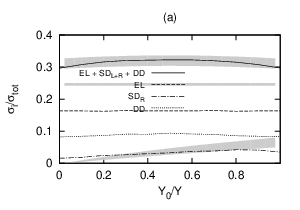
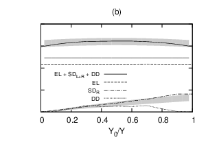
In figure 9 we show the ratio of the total diffractive, single diffractive and elastic cross sections to the total cross section at 1.8 TeV as a function of the Lorentz frame used. Figure 9a shows the result obtained with the initial proton wavefunction in eq. (8), while figure 9b shows the upper limit obtained by integrating over the initial proton wavefunctions after taking the square in eqs. (25)-(27). In these figures we also show results from the CDF collaboration (not including double diffraction).
The results in figure 9a do not agree well with the data. The elastic cross section is too low. The single diffractive cross section does not go to zero when . In this limit and there should be no phase space for diffractive excitation. The double diffractive excitation is about 9%, which is unrealistically high, and this cross section should also approach zero in the limits or . All these features illustrate the problems with our initial proton wave function, discussed above. This formalism presumes that there are other hadronic states, which have wavefunctions orthogonal to the proton wavefunction, and which have approximately the same mass. The limiting results in fig 9b, obtained when the fluctuations in the initial proton wave function are neglected, do not have this problem. We also see that these results agree quite well with the experimental estimates, supporting the assumption that the initial wavefunction fluctuations have a small effect compared to the fluctuations in the cascade evolution and the impact parameter dependence.
For the elastic cross section we also note (as was claimed above) that it is approximately frame-independent, as it should be. The upper limit shown in figure 9b is around 22%, which agrees well with the value ()% from E811 [35], while the value from CDF, ()% [34] is a bit larger.
The single diffractive cross section () is increasing (decreasing) when is increased, and in the model we make the identification of the diffractive masses:
| (40) |
where for 1.8 TeV we have . In figure 9 we also show results obtained from the CDF parameterization of single diffractive excitation [33]:
| (41) |
with mb, , and . Similar results are also presented by the E710 collaboration [36], although with somewhat larger errors. Our results in figure 9b agree quite well with the data, even if they are a little high for the largest excited masses. Besides not going to 0 when , the result in figure 9a also has a much too slow variation with , meaning a too low value for .
For double diffraction our result for , which corresponds to a central gap, is 2.0 mb. Experimental data exist for 900 GeV from the UA5 collaboration at the CERN Spp̄S collider [37]. Our result at this energy is 1.8 mb, which is consistent with the experimental result mb. Our results can also be compared to the model of Goulianos [38], who argues that should decrease with energy, due to saturation effects, from around 1.6 mb at 900 GeV to around 1.3 mb at 1.8 TeV. We also note that our result is consistent with a factorized dependence on the two masses, as expected from Regge formalism:
| (42) |
where denotes the distribution for single diffraction in eq. (41). (Note that double diffraction is not included in the CDF data in figure 9.)
As seen in figure 2 the same total cross section can be obtained with different sets of values for and . In figure 10 we see that varying these parameters, keeping constant, does modify the elastic cross section somewhat. However, our upper limit is still close to the data, leaving little room for a contribution from the initial proton wave function.

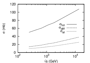
Finally we show in figure 11 the energy dependence of the total, the total diffractive (including elastic scattering), and the elastic cross sections, including our predictions for the LHC. (The values presented correspond to those in fig 9b, i.e. to the more realistic results obtained neglecting the fluctuations in the initial proton wave function.) The diffractive cross section is calculated in the cms with , which demands a central gap and implies that the diffractive excitations are limited by . The values we predict for the LHC are 108, 38, and 26 mb respectively.
4.2 Diffraction at HERA
Diffractive excitation has been measured at HERA by the ZEUS [39] and H1 [40] collaborations with two different methods. One is based on an observed rapidity gap. The ZEUS data obtained with this method [39] give the cross section integrated over all diffractively excited protons with mass GeV. Assuming that the contribution from events where the proton is excited beyond this limit is small, and can be neglected, the result of this method for corresponds to our model calculations for at :
| (43) |
The results are shown in figure 12 and we see a very good agreement with data, although there is a tendency for our cross sections to decrease a bit too slowly with .


The cross section for single diffractive excitation of the photon can also be calculated in our model, and in figure 13 we present the ratio wrt. the total diffractive cross section as a function of for different and . In [39] the ZEUS collaboration estimated this ratio to be , by comparing a parameterization33 3 Using a modified version of the model in [41]. of their diffractive data to results from their leading proton spectrometer. This result is obtained using the assumption that the ratio is independent of , and . Comparing with figure 13 we find that our result is consistent with the ZEUS number, but that we predict that the ratio actually does have a small dependence on and .


5 Conclusions and Outlook
We have in earlier papers presented an extension of Mueller’s dipole cascade model, which includes subleading effects from energy conservation and running coupling as well as colour suppressed effects from pomeron loops. The model is also implemented in a MC simulation program, which simplifies the comparison between theoretical ideas and experimental data, and allows more detailed studies of important non-leading effects. Calculations of total cross sections agree very well with experimental results for collisions and deep inelastic electron scattering.
To gain further insight into small- evolution and saturation, we have in this paper first presented a number of improvements of the model, in particular related to the confinement mechanism, and thereafter applied the model to elastic scattering and diffractive excitation, where we specifically study the effects of different sources for fluctuations.
A consistent treatment of confinement effects is achieved by replacing the infinite range Coulomb potential in the dipole splitting and in the dipole–dipole scattering with a screened Yukawa potential. By equating the screening length, , with the size of the proton entering into its wavefunction, we were able to get a good, boost-invariant description of the and total cross sections for a wide range of energies, using basically only two parameters, and . This new treatment of confinement has effects on the boost invariance of the model, further improving the earlier, almost frame independent, results.
Our treatment of diffraction is based on the formalism of Good–Walker and Miettinen–Pumplin. The cross sections for elastic scattering and diffractive excitation are here determined by the fluctuations in the interaction probability between different events. Contrary to other calculations, we can in our model easily consider all different sources for such fluctuations; those stemming from the dipole cascade evolution, the dipole–dipole scattering, from the impact parameter dependence, and from the initial photon and proton wavefunctions. We find that all of these sources give important contributions, apart from the initial proton wavefunction, and together they give a very good description of data on elastic and single- and doubly-diffractive scattering in both and collisions. We must, however, admit that we do not have a realistic quantum-mechanical description of the proton state in terms of dynamical variables. Here data are best reproduced if the contribution from the fluctuations in the initial proton state are small compared to the other contributions.
In a future publication we will use our model to study the quasi-elastic reactions and deeply inelastic Compton scattering (DVCS). In the future we also want to develop the model further to be able to describe exclusive multi-particle final states. This needs, however, a recipe for how to handle the virtual dipoles, those which do not participate in the collision and therefore cannot come on shell and give final state hadrons. To describe particle production in the proton fragmentation regions would also need a much improved description of the initial proton state.
References
- [1] T. Sjostrand and M. van Zijl Phys. Rev. D36 (1987) 2019.
- [2] UA8 Collaboration, R. Bonino et al. Phys. Lett. B211 (1988) 239.
- [3] CDF Collaboration, F. Abe et al. Phys. Rev. Lett. 79 (1997) 2636–2641.
- [4] D0 Collaboration, B. Abbott et al. Phys. Lett. B531 (2002) 52–60, hep-ex/9912061.
- [5] ZEUS Collaboration, M. Derrick et al. Phys. Lett. B315 (1993) 481–493.
- [6] H1 Collaboration, T. Ahmed et al. Nucl. Phys. B429 (1994) 477–502.
- [7] K. Golec-Biernat and M. Wusthoff Phys. Rev. D59 (1999) 014017, hep-ph/9807513.
- [8] K. Golec-Biernat and M. Wusthoff Phys. Rev. D60 (1999) 114023, hep-ph/9903358.
- [9] A. H. Mueller Nucl. Phys. B415 (1994) 373–385.
- [10] A. H. Mueller and B. Patel Nucl. Phys. B425 (1994) 471–488, hep-ph/9403256.
- [11] A. H. Mueller Nucl. Phys. B437 (1995) 107–126, hep-ph/9408245.
- [12] E. Iancu, G. Soyez, and D. N. Triantafyllopoulos Nucl. Phys. A768 (2006) 194–221, hep-ph/0510094.
- [13] M. Kozlov, E. Levin, and A. Prygarin hep-ph/0606260.
- [14] E. Avsar, G. Gustafson, and L. Lönnblad JHEP 07 (2005) 062, hep-ph/0503181.
- [15] E. Avsar, G. Gustafson, and L. Lonnblad JHEP 01 (2007) 012, hep-ph/0610157.
- [16] M. L. Good and W. D. Walker Phys. Rev. 120 (1960) 1857–1860.
- [17] Y. Hatta, E. Iancu, C. Marquet, G. Soyez, and D. N. Triantafyllopoulos Nucl. Phys. A773 (2006) 95–155, hep-ph/0601150.
- [18] G. P. Salam Acta Phys. Polon. B30 (1999) 3679–3705, hep-ph/9910492.
- [19] J. R. Andersen Phys. Lett. B639 (2006) 290–293, hep-ph/0602182.
- [20] B. Andersson, G. Gustafson, and J. Samuelsson Nucl. Phys. B467 (1996) 443–478.
- [21] G. Gustafson and G. Miu Eur. Phys. J. C23 (2002) 267–274, hep-ph/0110143.
- [22] B. Andersson, G. Gustafson, and H. Kharraziha Phys. Rev. D57 (1998) 5543–5554, hep-ph/9711403.
- [23] E. Avsar and G. Gustafson JHEP 04 (2007) 067, hep-ph/0702087.
- [24] E. Avsar arXiv:0709.1371 [hep-ph].
- [25] I. Balitsky Phys. Rev. D75 (2007) 014001, hep-ph/0609105.
- [26] Y. V. Kovchegov and H. Weigert Nucl. Phys. A789 (2007) 260–284, hep-ph/0612071.
- [27] I. Balitsky. Talk presented at the ISMD07, Berkeley, August 2007, see http://www-rnc.lbl.gov/ISMD/.
- [28] H. I. Miettinen and J. Pumplin Phys. Rev. D18 (1978) 1696.
- [29] H. Kowalski and D. Teaney Phys. Rev. D68 (2003) 114005, hep-ph/0304189.
- [30] S. Sapeta and K. Golec-Biernat Phys. Lett. B613 (2005) 154–161, hep-ph/0502229.
- [31] A. H. Mueller and G. P. Salam Nucl. Phys. B475 (1996) 293–320, hep-ph/9605302.
- [32] G. P. Salam Nucl. Phys. B461 (1996) 512–538, hep-ph/9509353.
- [33] CDF Collaboration, F. Abe et al. Phys. Rev. D50 (1994) 5535–5549.
- [34] CDF Collaboration, F. Abe et al. Phys. Rev. D50 (1994) 5550–5561.
- [35] E811 Collaboration, C. Avila et al. Phys. Lett. B445 (1999) 419–422.
- [36] E710 Collaboration, N. Amos et al. Phys. Lett. B301 (1993) 313–316.
- [37] UA5 Collaboration, R. E. Ansorge et al. Z. Phys. C33 (1986) 175.
- [38] K. Goulianos Phys. Lett. B358 (1995) 379–388.
- [39] ZEUS Collaboration, S. Chekanov et al. Nucl. Phys. B713 (2005) 3–80, hep-ex/0501060.
- [40] H1 Collaboration, C. Adloff et al. Z. Phys. C76 (1997) 613–629, hep-ex/9708016.
- [41] J. Bartels, J. R. Ellis, H. Kowalski, and M. Wusthoff Eur. Phys. J. C7 (1999) 443–458, hep-ph/9803497.