Efficient Algorithms for Node Disjoint Subgraph Homeomorphism Determination
Abstract
Recently, great efforts have been dedicated to researches on the management of large scale graph based data such as WWW, social networks, biological networks. In the study of graph based data management, node disjoint subgraph homeomorphism relation between graphs is more suitable than (sub)graph isomorphism in many cases, especially in those cases that node skipping and node mismatching are allowed. However, no efficient node disjoint subgraph homeomorphism determination (ndSHD) algorithms have been available. In this paper, we propose two computationally efficient ndSHD algorithms based on state spaces searching with backtracking, which employ many heuristics to prune the search spaces. Experimental results on synthetic data sets show that the proposed algorithms are efficient, require relative little time in most of the testing cases, can scale to large or dense graphs, and can accommodate to more complex fuzzy matching cases.
1 Introduction
Recently, large scale graph based data management has received more and more research attentions, due to the broad application of graph based data. In the study of graph based data management, graph based pattern matching, i.e., to determine whether the structure of a pattern graph can match to that of a data graph, is the key of many problems about graph data management.
Existing graph pattern matchings can be classified into two preliminary categories: exact matching and inexact matching. Exact matching requires that the matched two graphs are isomorphic to each other; i.e., exact graph pattern matching is based on graph isomorphism relations between graphs. While the inexact graph matching is often considered as subgraph isomorphism between graphs, which means that pattern graph matches to data graph if and only if is subgraph isomorphic to .
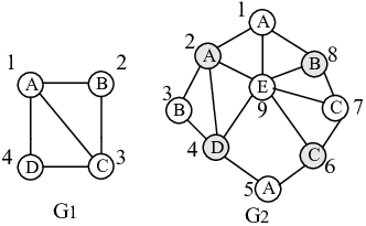
However, in real applications, inexact graph pattern matching based on subgraph isomorphism cannot represent the fuzzy matching in some cases that node skipping or node mismatching is allowed. For example, as shown in Figure 2, although is not a subgraph of , still can be regarded as matched to if node skipping or node mismatching is allowed. In other words, is matched to from the abstract topological structure perspective, because retains the abstract topological structure of if paths in can be contracted into the corresponding edges in .


However, this kind of fuzzy matching is more desired in many real applications than subgraph isomorphism based inexact matching. For instance, the discovery of frequent conserved subgraph patterns from protein interaction networks [1, 2] is an important and challenging work in evolutionary and comparative biology, where ’conserved’ just means the inexact graph pattern matching allowing node mismatch and node skipping. Similarly, in social network analysis, the direct connection between nodes usually is not the focus; instead, the high-level topological structure with independent paths contracted is of great interest.
Using Graph Minor theory [4], the abstract topological structure in many real applications can be described as topological minor, and the relation between abstract topological structure and its detailed original graph can be described as node/vertex disjoint subgraph homeomorphism. However, to determine whether a pattern graph is a topological minor of data graph is not a trivial thing, and this problem has been proved to be NP-complete when and are not fixed [3]. Although Robertson and Seymour [4] have proposed a framework to solve minor containment problem that is a generalization of topology containment problem and [5] has implemented the framework, no efficient algorithms have been dedicated to solve ndSHD (in other contexts, also known as topological minor containment, homeomorphic embedding or topological embedding), to the best of our knowledge.
To efficiently determine the node disjoint homeomorphism relation between two graphs, we propose two algorithms based on state space searching with backtrack, which integrate many heuristics into the searching procedure to prune the search spaces. The work in the paper is inspired by Ullmann’s [6] s̱ubgraph i̱somorphism ḏetermination (SID) algorithm. However, for ndSHD, we need to do some more specific things. First, for ndSHD, not only node mapping space but also edge-path mapping space needs to be searched, whereas for SID only the former needs to be searched. Second, for ndSHD, according to the definition of topological minor, we need to perform pairwise independence determination of the paths to ensure the paths are disjoint. Third, for SID, only edge information is explored, while in ndSHD path information is explored too, which will be a great challenge to the efficiency of the algorithm since the amount of paths is exponential to the size of the graph.
In a summary, we make the following contributions in this paper:
- 1.
We propose two efficient algorithms for node disjoint subgraph homeomorphism determination. To the best of our knowledge, it’s the first paper dedicated to design practical efficient algorithms for node disjoint subgraph homeomorphism determination or topological minor containment determination problem.
- 2.
We investigate the properties of topological minors, and employ these properties as the heuristics to prune the search space.
- 3.
We present a systematic performance study of proposed algorithms. The experimental results show that the algorithms are efficient and scalable on synthetic data sets.
2 Preliminaries
We begin with some basic notations that are used in [7]. Let be a vertex labeled graph, where is the set of vertices, is the set of edges and , and is a label function , giving every vertex a label.(In this paper, we only focus on vertex labeled graphs. Unlabeled graph can be considered as a labeled graph with all vertexes having the same vertex label.) The vertex set of is referred to as , and its edges set as . A path in a graph is a sequence of vertices ,,…,, where and . The vertices and are linked by and are called its ends. The number of edges of a path is its length, and the path of length is denoted as . A path is simple if its vertices are all distinct. Particularly, a group of paths are independent if none of the paths have an inner vertex on another path. In the other words, a path intersecting with other paths only at its ends can be called as an independent path. Be aware that the independent paths are the key to study topological minors of a graph.
2.1 Topological Minor
As described in [7], a topological minor of a graph is obtained by contracting the independent paths of one of its subgraphs into edges. For example, in Figure 2, is a topological minor of , since can be obtained by contracting the independent paths of which is a subgraph of . Clearly, contracting independent paths helps simplify a (sub)graph without compromising its abstract topological information.
Formally, as shown in Figure 2, if we replace all the edges of with independent paths between their ends, so that these paths are pairwise node independent, namely none of these paths has an inner vertex on another path, then is a subdivision of , denoted as . If is a subgraph of , then is a topological minor of . As a subdivision of and a subgraph of , if is obtained by replacing all the edges of with independent paths with length from to , then is a (l, h)-subdivision of and is a (l, h)-topological minor of .
Given two graph and , if is a topological minor of , then there exists a corresponding node disjoint subgraph homeomorphism from into , which is a pair of injective mappings from into , where is an injective mapping from vertex set of into that of and is an injective mapping from edges of into simple paths of such that (1) for each , is a simple path in with and as two ends;(2) all mapped paths are pairwise independent. In other words, if is node disjoint subgraph homeomorphic to , all the edges of can be mapped to a corresponding simple path of and all the mapped path are pairwise independent; all the nodes in can be mapped to a corresponding node in (all the mapped nodes are called branch nodes of ).
2.2 Problem Definition
As shown in Figure 4, given two vertex labeled graphs and , given the minimal path length and the maximal path length , the problem is whether is a -topological minor of , i.e., is node disjoint homeomorphic to so that all mapped paths in have length from to . Obviously, this problem is a typical determination problem. When the answer is true, the homeomorphism mapping also can be obtained. The solution to the determination problem also can be extended to solve the enumeration problem, which is to find the entire valid homeomorphism mappings between two graphs.
The answer to the problem is sensitive to the given parameter . For example, in Figure 3, if is , which means the edges in can only be mapped to the paths in with length , then nodes in can be mapped to the four nodes in shadow in and the five edge-path mappings are . If is , is not a topological minor of . The influence of parameter on topology containment determination has been discussed in [8] in detail.

3 Algorithm Framework
To simplify the description of the algorithm, we first give some notations. Assume that vertex labeled graph is a -topological minor of vertex labeled graph under the node disjoint subgraph homeomorphism , where and , the image of under mapping is denoted as . The number of vertices and edges of and are , and , , respectively. For the convenience of notation, we call as minor graph, and as data graph; without explicit statement, in the following discussion, always denote a minor graph, always denote a data graph.
3.1 A Rudimentary Algorithm
To determine whether is a topological minor of is equivalent to find a pair of mapping between these two graphs. The mapping maps the nodes in to the nodes with the same label in so that can map each edge of to a corresponding path in . Obviously, the final solution of the determination, i.e., the complete mapping between these two graphs, can be described as ,where is the node match set and is the edge-path match set. All the mapped nodes of can be denoted as , and all the mapped paths of can be denoted as .
The process of finding the homeomorphism mapping can be suitably described by means of State Space Representation [9]. Each state of the matching process can be associated with a partial mapping solution , where and are the node match set and edge-path match set at state , respectively. Obviously, contains all the matches we have found so far and probably become a subset of some final match set .
Given the two vertex labeled graphs as shown in Figure 3, a naive two level state space searching procedure for a topological mapping is shown as Figure 4, where the first level is to find a suitable node mapping solution (shown in the dotted box of Figure 4(a)) and the second level is to find a suitable edge-path mapping solution (shown in the dotted box of Figure 4(b)). The corresponding algorithm framework is shown as follows.
Algorithm
ndSHD1(,,,)
Input: ,:vertex labeled graphs; :minimal
path length; :maximal path length.
Output: If is a -topological minor of
return true and return the first found
node disjoint subgraph homeomorphism , otherwise return
false.
- 1.
Initial();/*Initialize SHD, Generate necessary path information, Initialize the basic data structures*/
- 2.
Initial();
- 3.
; /*initialize state as empty state*/
- 4.
NodeMappingSearch(,,); /*node mapping space search*/
- 5.
if not IsValid()
- 6.
return false;
- 7.
else
- 8.
EdgePathMappingSearch(); /*edge-path mapping space*/
- 9.
if not IsValid()
- 10.
return false;
- 11.
else
- 12.
return true;
At first, we initialize two basic data structures : node compatible matrix and independent path matrix as well as its associated path indexed structure. Then we start the node matching process from the empty state. Each time we select a branch in the state space, a state transits to a new successor state ’ by adding a new match, which is a node pair or an edge path pair, to the partial solution. Each time a new match state arrives, and are updated so that the node mapping space and edge-path mapping space can be pruned. When a complete node mapping has been found, the matching process will come to the second level: edge-path matching space search. Similar to the search process in node mapping space, each time a branch is selected, an edge-path pair is added to the partial mapping solution and the independent path matrix is updated. The process continues until a complete edge-path mapping is found.
In the above searching process, if all the possible valid branches in the subspace rooted at current state have been explored, but still no valid match can be found, the searching process backtracks to the parent state of . And any time the procedure enters into dead state which will be discussed in 3.5, the whole process will stop and return false which means the two graphs do not satisfy the -topological minor relationship.
3.2 Basic Data Structure
As described above, we need to two basic data structures, one is used to represent the node mapping information; the other is used to represent independent path information of . For the former, we use node compatible matrix; the latter, we use independent path matrix as well as a path index structure. Both of them are changing with the transition of the matching state.


We define node compatible matrix to be a (rows) (columns) matrix whose elements are ’s or ’s. At the final success state, we can get a final mapping matrix whose elements are ’s or ’s, such that each row contains exactly one and each column contains no more than one . The final mapping matrix represents a valid one to one mapping between nodes of and , while the initial compatible matrix represents the probable mappings between nodes of and . The initial node mapping and the final node mapping between and in Figure 3 is shown in Figure 5. Obviously for each element of , .
Clearly, to reduce the number of ’s in is the key to speed up the search procedure in node mapping space. Hence, the first key step is to construct an initial compatible matrix with as less ’s as possible. For this reason, we first introduce Lemma 1. Due to the limitation of space, the detailed proof is omitted in this paper.
Lemma 1
The number of elements of the independent path set starting from a specified vertex is no more than , where denotes the degree of .
Since every path set starting from necessarily pass through one or more edges incident with , the independent path set starting from has at most elements. According to lemma 1, the node in cannot be matched to those nodes in whose degree is less than . Therefore, we construct the initial compatible matrix in accordance with the following rule: if , otherwise . As shown in Figure 3, in cannot mapped to of , although these two nodes have the same label.
When constructing Independent Path Matrix and its associated Path Indexed Structure, the first problem we face is whether we need to generate all the path information of . The answer is false, which is based on the following lemma.
Lemma 2
If is a -topological minor of under subgraph homeomorphism , then only contains paths ending with those branch nodes in .
For example, in Figure 3, since in cannot be a branch node, then all paths starting from needn’t to be enumerated. However, note that the path having as inner vertex can not be ignored.
Therefore, we only need to enumerate all the paths between all candidate branch node pairs. These candidate branch nodes can be filtered out by matrix . As shown in Figure 4, since column and have only ’s, and in cannot be branch nodes, thus could be filtered out and the remaining nodes in are just candidate branch nodes. The cardinality of the candidate branch node set is denoted as .
Then, we can define the independent path matrix to be
(rows)
(columns) matrix whose
elements are positive integers or ’s, which represent the number
of paths between the node pair in .
The corresponding detailed path information are stored in a list
array RLists, where each list in RLists contains
corresponding path addresses that point to the physical storage of
the path. RLists can be considered as a path index structure that is
built according to the end vertex pair of the path.
3.3 State Space Searching
The procedure of node mapping space searching and edge-path mapping space searching are similar to each other. These two procedures are shown as follows.
Algorithm Node/EdgePatbMappingSearch1
(,,)
Input: :the
current matching state; :the current node compatible matrix; :
the current independent path matrix.
Output: found: a boolean variable indicating whether
a complete node/edge-path mapping has been found.
- 1.
if( is dead state)
- 2.
return false;
- 3.
if( is complete mapping state)
- 4.
return true;
- 5.
let foundfalse
- 6.
while(not found && Exists Valid node/edge-path Mapping Pair)
- 7.
GetNextNodePair(); /*GetNextEdgePathPair();*/
- 8.
BackupState();
- 9.
; /**/
- 10.
Refine(,);
- 11.
foundNode/EdgePathMappingSearch(, , );
- 12.
if(found)
- 13.
return true;
- 14.
else
- 15.
RecoverState();
- 16.
return false;
From line 1-2, we can see that when a new state arrives, can be a dead state or success state(complete mapping state). The state space search arrives at a success state if all the node mappings or edge-path mappings have been found, which means or , where and are the node match set and edge-path match set at state . The node mapping state space search arrives at a dead state if there is a row with all ’s in node compatible matrix of the current state, i.e. ,s.t. . And the edge-path mapping state space search arrives at a dead state if there is no path between any one branch node pairs, i.e., ,s.t. , where gets the vertex corresponding to the th column in matrix , which can be easily determined from independent path matrix of the current state.
Any time the search process enters into a success state or dead state, the procedure is over. If success state arrives, the complete mapping is found and the procedure returns true. If dead state arrives, the procedure returns false. On any other cases, the procedure will continue exploring the state space. The 1-11 lines describe the process.
Assume the process comes to a state that is only a partial solution. Then as long as there exists a valid mapping pair, i.e., a node pair or an edge-path pair, we need to generate a new state by adding the new match (line 9) to the existing solution . To enable backtracking, we need to backup the current state first (line 8), including the node compatible matrix, independent path matrix etc. Because after a new match added to the current solution, these two basic data structure will be refined to prune the following mapping space (line 10). Then DFS continues, until the search enters into dead state or success state. If we cannot find a success state in subtree space rooted at , we recover the state (line 15), and try the sibling state branches.
3.4 Refinement Procedure
To traverse all possible mapping branches is time consuming, so space pruning is essential for ndSHD. For this purpose, we devise two refinement procedures on and , respectively, the correctness of the former refinement is based on Lemma 3,4, and the latter is based on Lemma 5.
Lemma 3
In the matching process, let be the current state, if and will be a partial solution of some final solution , then any path with as inner vertex will not .
If and will be a subset of some final solution, then will a branch nodes of . Since branch nodes can only be the end vertex of the final independent path set, thus any path with as inner vertex will not belong to the final independent path set.
Lemma 4
In the matching process, let be the current state, if and will be a partial solution of some final solution , then any path passing trough the inner vertex of will not .
Obviously, if , then all the path passing through any inner vertex of will joint with , so all these paths will not occur in .
Lemma 3 implies that, if a vertex in is added to the existing node match set, all the paths with as inner vertex can be removed from RLists and the number in the corresponding element in can be decreased. Lemma 4 implies that if we reach a new state by adding a new edge-path pair , all the path passing through any inner vertex of can be removed from RLists and the number in the corresponding element in can be reduced.
As shown in Figure 4, if vertex in is mapped to in , any path passing through could be removed from RList, thus the potential edge-path mapping space could be pruned. As shown in Figure 4, when is added to the partial solution, the subtree rooted at node will be reduced, in the way that all the branches containing paths passing through vertex will be pruned.
Lemma 5
In the matching process, let be the current state, if and will be a partial solution of some final solution , then the following statements hold true:
- 1.
and .
- 2.
such that and and .
- 3.
The path set consisting of the paths to which all mentioned ’s in (1) and (2) indicate is independent.
In the above statements, the function gets an index in for a node in ; and obtains the adjacent nodes set of .
Suppose that the partial solution of current state will grow to be one final successful solution, Lemma 5 implies that two node and is compatible if only the three conditions are satisfied, i.e., if any one is not satisfied, in node compatible matrix at state , namely , could be refined to be 0.
As shown in Figure 4, assume current matching state is , and . Condition 1 implies that if (3,7) can be added to , i.e., in can be mapped to in , there must exist two independent paths from to and in , otherwise can be refined to be , thus the node mapping space could be pruned. Moreover, since and are adjacent in , there must exist a corresponding path in from to some node with the same label as of , otherwise can be refined to be , which is stated in condition 2. Furthermore, all the above paths must be node disjoint, which is implied in condition 3. Obviously, if is set as (2,2), paths connecting to , and all pass through node . Hence in matrix can be refined to be .
3.5 More Efficient Searching Strategy
A basic observation of the above refinement procedures is that the constraint resulting from an edge-path match will be more restricted than that resulting from a node match. Hence, a better strategy is to try edge-path match as early as possible, instead of performing edge-path match only after complete node match has been found. We denote these two strategy as (old strategy) and (new strategy), respectively; and algorithms employing two strategies are denoted as ndSHD1 and ndSHD2, respectively. Intuitively, in ndSHD2 the searching procedure will meet with the dead state very early if the current searching path will not lead to a successful mapping solution, thus the searching procedure will fast backtrack to try another mapping solution.
As an example, assume that is set as (2,2) and the current matching state is such that . Since and is adjacent in , why we not try to match a path in for the edge ? If we do so, there are only two suitable edge-path pairs and . Then, once has been added to , all paths in passing through will be excluded from and , thus the searching space could be pruned early. Furthermore, we can see that the current partial mapping solution will not be a part of a final successful solution, thus any other solution with this partial solution as subset will be pruned. And if we try the edge-path pair , we can eventually find a successful complete mapping solution.
The framework of the ndSHD2 is similar to that of ndSHD1, which is omitted here. The detailed procedure of ndSHD2 is shown in NodeMappingSearch2 and EdgePatbMappingSearch2. Note that, in NodeMappingSearch2, after a new node match has been added to , we can get an edge set consisting of edges that connect to any vertex exiting in (line 11), namely . If (for connected graph, it only happened at the initial stage of the first node match), we continue the node mapping searching procedure (line 12-13); otherwise, we switch to edge-path mapping search procedure to find valid path in for each edge in (line 14-15). In EdgePatbMappingSearch2, if we can find valid paths for all the edges in E, the edge-path mapping search procedure returns true (line 3-4) and we will turn to the node mapping space search (line 13); otherwise, we continue the edge-path mapping search procedure (the while body).
Algorithm NodeMappingSearch2
(,,)
Input and
Output is the same as that in NodeMappingSearch1.
- 1.
if( is complete mapping state)
- 2.
return true;
- 3.
if( is dead state)
- 4.
return false;
- 5.
let foundfalse
- 6.
while(not found && Exists Valid node Mapping Pair)
- 7.
GetNextNodePair(); /*Get a next valid node pair*/
- 8.
BackupState();
- 9.
;
- 10.
Refine(,);
- 11.
NewEdgeEmergent(,)
- 12.
if
- 13.
foundNodeMappingSearch2(, , );
- 14.
else
- 15.
foundEdgePathMappingSearch2(, , , );
- 16.
if(found)
- 17.
return true;
- 18.
else
- 19.
RecoverState();
- 20.
return found;
Algorithm EdgePathMappingSearch2
(,,,)
Input and
Output is the same as that in EdgeMappingSearch1 except
, which is the edges in induced by .
- 1.
if( is dead state)
- 2.
return false;
- 3.
if( is complete mapping state with respect to E)
- 4.
return true;
- 5.
let foundfalse
- 6.
while(not found && Exists Valid edge-path Mapping Pair)
- 7.
GetNextEdgePathPair(); /*Get a next valid edge-path pair*/
- 8.
BackupState();
- 9.
;
- 10.
Refine(,);
- 11.
foundEdgePathMappingSearch2(, , , );
- 12.
if(found)
- 13.
foundNodeMappingSearch2(, , );
- 14.
else
- 15.
RecoverState();
- 16.
return false;
4 Experimental Evaluation
To test the efficiency of the algorithm, we generate the synthetic data sets according to the random graph [10] model that links each node pair by probability . All generated graphs are vertex labeled undirected connected graphs. We also randomly label every node so that the vertex labels are uniformly distributed. We implement the algorithm in C++, and carry out our experiments on a Windows 2003 server machine with Intel 2GHz CPU and 1G main memory.
The efficiency of the algorithms is influenced by the following factors: : node size of , : node size of , : average degree of , : average degree of , : the minimal and maximal path length. The efficiency also can be influenced by the number of vertex labels. Obviously, large number of labels will exert great constraint on the initial node compatible matrix, thus reduce the runtime significantly. However, for determination algorithms, the runtime also may be influenced by the answer to the determination. Generally, if the answer is false, in the worst case the algorithm may need to traverse the entire mapping spaces, which is very time consuming. If the answer is true, then in the best case the algorithm may only need to try one complete match procedure. However, in the following experiments, we can see that result of the determination has limited impact on the runtime, which could partly be attributed to the strong pruning ability of the refinement procedure. Due to these pruning techniques, even the result is false, the procedure will backtrack as early as possible, thus the whole runtime is rarely impacted.


First we will demonstrate the scalability with respect to the growth of the size of nodes of data graph via experiment . We use a complete graph with 4 uniquely labeled nodes, denoted as , as a minor graph; we generate overall 200 data graphs with node size varying from to in an increment of 20. The average degree of each data graph is fixed as 4 and nodes of each graph are randomly labeled as one of overall 20 labels. and are fixed as 1 and 3, respectively, meaning that the path length is in the range of . Thus the parameters can be denoted as . From Figure 7, we can see that ndSHD1 and ndSHD2 both are approximately linearly scalable with respect to the number of nodes in , irrespective of the result of the determination result. Notice that for with about nodes and edges, the worst case of ndSHD1is no more than s, the worst case of ndSHD2 is no more than s.
is designed to show the scalability of ndSHD1 and ndSHD2 with respect to the size of , where we fix some parameters as and vary the size of from 6 to 82 in increment of 4 to generate 20 minor graphs. Each minor graph is uniquely labeled, meaning that the number of labels equals to that of nodes. Two data graphs are used, one has average degree as 8 and the other as 20. These two data graphs are randomly labeled as one of 200 labels. Figure 9(a) and (b) show the results with set as and , respectively; and these two experiments are denoted as and , respectively. The determination results of running case shown in Figure 9(a) are all false due to the relative sparsity of ; and determination results of all running cases shown in Figure9(b) are true due to relatively higher density of . As can be seen, ndSHD1 and ndSHD2 both are approximately linearly scalable with respect to the number of nodes in . We also can see that, when is sparse, the difference of performance between ndSHD1 and ndSHD2 are so minute that can not be discerned; whereas as becomes denser, running time of ndSHD1 is not available, meaning that all running cases need time larger than one hour, while runtime increase of ndSHD2 is not very substantial.


is designed to show the scalability with respect to the growth of density of , parameters are fixed as . Minor graph are uniquely labeled; data graphs are randomly labeled as one of 20 labels. Table 1 shows the running time when we vary from 2 to 20 in increment of 1. As can be seen, runtime of ndSHD1 and ndSHD2 both approximately increase linearly with the growth of . However, we must note that for ndSHD1, there exists some outliers which consume too much time, e.g, when , more than 10 minutes are needed, when running time is not available. Compared to ndSHD1, ndSHD2 is more stable.
| 2 | 3 | 4 | 5 | 6 | 7 | 8 | 9 | 10 | 11 | |
| 0 | 0 | 0 | 0 | 1 | 1 | 1 | 1 | 1 | 1 | |
| 0 | 0.14 | 0.31 | 1.78 | 21.67 | 19.69 | 1.77 | 1.23 | 83.66 | 661.33 | |
| 0.016 | 0.14 | 0.33 | 1.05 | 11.41 | 0.97 | 0.92 | 1.27 | 2.14 | 3.77 | |
| 12 | 13 | 14 | 15 | 16 | 17 | 18 | 19 | 20 | ||
| 1 | 1 | 1 | 1 | 1 | 1 | 1 | 1 | 1 | ||
| 3.23 | 3.89 | 4.24 | 5.36 | - | 6508.7 | 7.75 | 10.06 | 9.77 | ||
| 3.11 | 3.92 | 4.23 | 5.36 | 6.66 | 7.91 | 8.06 | 10.72 | 10.11 |
Figure 9 shows the runtime of the algorithm with respect to . Parameters of this experiment (denoted as ), are set as . The vertex labeling of minor graph and data graphs are the same as . As can been seen the broader the range is, the longer the running time is; and the runtime of ndSHD1 and ndSHD2 both increase dramatically with the growth of upper bound of path length. However, the increasing speed of ndSHD2 is slower than that of ndSHD1, which implies that ndSHD2 is more efficient than ndSHD1 with respect to larger . The super linearly growth of the runtime with the increase of upper bound of the path length can be partly attributed to the exponentially growth of the number of potential mapped paths. Luckily, in the real applications, larger upper bound is too unrestricted when performing fuzzy matching on graph data, thus usually upper bounds less than 3 are used.

To examine the impact of number of vertex labels on the performance of ndSHD1 and ndSHD2, we use a uniquely labeled graph with 6 nodes and 15 edges as minor graph, a graph with 1000 nodes and 4000 edges as data graph. We randomly labeled the data graph from 10 labels to 200 labels in increment of 10 to generate 20 different labeled data graphs. and are set as 1 and 3, respectively. The result of this experiment (denoted as ) is shown in Figure 10. Clearly, runtime of ndSHD1 and ndSHD2 substantially decrease with the growth of number of labels of , which confirms to what we have expected, since larger number of labels in can reduce the node mapping space between minor graph and data graph. We also can see that ndSHD2 outperforms ndSHD1 to a great extent when label number is small.
To examine the stability of ndSHD1 and ndSHD2, we recorded in Table 2 the statistics including max, mean and standard deviation of sample data used in the above experiments. We can see that in almost all the experiments, the standard deviation of ndSHD2 is much less than that of ndSHD1, indicating that ndSHD2 is more stable than ndSHD1.
In a summary, in some simple running cases, such as small size of minor graph, sparse data graphs, small value of upper bound of path length, larger number of labels in data graphs, both ndSHD2 and ndSHD1 are scalable and efficient. However, in more complex cases, ndSHD2 will outperform ndSHD1 substantially in all aspects, including scalability, efficiency and stability.
In Figure 11,we also illustrate the detailed searching procedure of two running cases to show the superiority of ndSHD2 to ndSHD1. In both of these two cases, ndSHD2 runs much faster than ndSHD1. Since the mapping searching procedure has been designed to be a recursive procedure, statistics about the recursive depth of each match (node-node match or edge-path match) will be a significant index indicating the performance of the algorithm. Hence, we recorded recursive depth of all matches in the searching procedure. Obviously, either narrow width of the exploring space or small value of the average backtrack depth, will lead to the less runtime of the algorithm. Hence ,from Figure 11, we can easily see the great advantage of ndSHD2 over ndSHD1, which can be attributed to the small value of the width or average backtrack depth in the actual exploring space.

| statistics | ||||||||||||
|---|---|---|---|---|---|---|---|---|---|---|---|---|
| max | 12.36 | 6.89 | 4.312 | 4.234 | - | 26.84 | 6509 | 11.41 | 33.44 | 12.56 | 107.9 | 6.297 |
| mean | 1.727 | 1.49 | 1.709 | 1.73 | - | 10.06 | 408 | 4.32 | 6.325 | 2.675 | 8.312 | 1.392 |
| std | 1.788 | 1.396 | 1.344 | 1.331 | - | 7.24 | 1530 | 3.797 | 13.34 | 4.937 | 24.89 | 1.909 |
5 Conclusions
In this paper, we investigated the problem known as node disjoint subgraph homeomorphism determination; and proposed two practical algorithms to address this problem, where many efficient heuristics have been exploited to prune the futile searching space. The experimental results on synthetic data sets show that our algorithms are scalable and efficient. To the best of our knowledge, no practical algorithm is available to solve node disjoint subgraph homeomorphism determination.
References
- [1] R.B.Kelley,et al, Conserved pathways within bacteria and yeast as revealed by global protein network alignment. PNAS,100(20): 11394-11399 ,2003
- [2] R.Sharan,et,al, Identification of protein complexes by comparative analysis of yeast and bacterial protein interaction data. RECOMB ¡¯04: p 282¨C289, 2004.
- [3] M.R. Garey, D.S. Johnson, Computers and Intractability. A Guide to the Theory of NP-completeness, W.H. Freeman and Company, New York, 2003.
- [4] Neil Robertson and P.D.Seymour: Graph minors. XIII: The disjoint paths problem, Journal of Combinatorial Theory. Vol.63 (1995) 65-110.
- [5] IIIya V.Hicks: Branch Decompositions and Minor Containment, Networks, Vol .43(1) (2004)1-9.
- [6] J.R.Ullmann: An Algorithm for Subgraph Isomorphism, Journal of the ACM, Vol.23(1976) 31-42.
- [7] Reinhard Diestel. Graph Theory, Springer-Verlag.(2000).
- [8] R. Jin, C.Wang, D. Polshakov, S. Parthasarathy, G. Agrawal: Discovering frequent topological structures from graph datasets. In KDD’05, Chicago,USA,(2005) 606-611.
- [9] N.J. Nilsson: Principles of Artificial Intelligence. Springer-Verlag,(1982).
- [10] P.Erdös and A.Rényi, On random graphs, Publicationes Mathematicae(1959)290-297.