Interaction Correction of Conductivity Near a Ferromagnetic Quantum Critical Point
Abstract
We calculate the temperature dependence of conductivity due to interaction correction for a disordered itinerant electron system close to a ferromagnetic quantum critical point which occurs due to a spin density wave instability. In the quantum critical regime, the crossover between diffusive and ballistic transport occurs at a temperature , where is the parameter associated with the Landau damping of the spin fluctuations, is the impurity scattering time, and is the Fermi energy. For a generic choice of parameters, is few orders of magnitude smaller than the usual crossover scale . In the ballistic quantum critical regime, the conductivity has a temperature dependence, where is the dimensionality of the system. In the diffusive quantum critical regime we get dependence in three dimensions, and dependence in two dimensions. Away from the quantum critical regime we recover the standard results for a good metal.
pacs
75.45.+j, 72.15.RnI Introduction
The effect of disorder and interaction on the temperature dependence of conductivity of metals has been a topic of theoretical and experimental investigations for over two decades. altshuler; aleiner1; zna However, most of these studies are on systems which are “good metals” that behave as Fermi liquids (FLs), for which the electron-electron interaction is short-ranged. More recently, the observation of anomalous transport properties of metals which are near putative quantum critical points (QCPs) stewart has inspired theorists to examine the interplay of disorder and interaction on transport properties of metals near quantum criticality. ipaul; kim; prl85; belitz2; rosch1
In contrast with good metals, the electron-electron interaction near a QCP can be long-ranged, which raises the possibility that in the latter case the combined effect of disorder and interaction strongly influences the temperature dependence of conductivity. From this perspective the study of charge transport near a ferromagnetic QCP is particularly interesting. ipaul Close to a ferromagnetic QCP of the spin density wave variety, the spin fluctuations are gapless (i.e., long ranged), but they do not break any lattice symmetry. As a result, the contribution to resistivity due to the inelastic scattering of the carriers with the spin fluctuations in a clean system (where effects of impurity can be neglected) is zero, unless Umklapp processes are taken into account in order to relax momentum. On the other hand, in a dirty system the “interaction” correction to the residual resistivity is expected to become important, especially at low enough temperature when the lattice mediated inelastic scattering with spin fluctuations is frozen out. The interaction correction is the result of quantum interference between semiclassical electron paths where, along one path electrons are scattered elastically by impurities and along the second path they are scattered by the self-consistent potential of Friedel oscillations. zna The study of the temperature dependence of conductivity due to this subtle quantum interference process for a system close to a ferromagnetic QCP is the topic of this paper.
From the point of view of experiments, the existence of a ferromagnetic QCP is currently a topic of investigation. In most three dimensional compounds, such as UGe2 huxley and ZrZn2, uhlarz the ferromagnetic transition from the paramagnetic state becomes first order as the Curie temperature is lowered by the application of pressure. In two dimensions the most promising candidate for exhibiting ferromagnetic type of quantum critical behaviour is the bi-layer material Sr3Ru2O7 which undergoes metamagnetic transition in the presence of an external magnetic field. grigera Until recently, it was believed that the metamagnetic transition in this material could be tuned to a quantum critical end point for which a spin fluctuation type of theory was considered appropriate. schofield However, recent experiments on cleaner samples reveal that the approach to the quantum critical end point is pre-empted by a new phase transition, whose origin is itself a subject of investigation currently. grigera2 On the other hand, the fact that this new phase transition in Sr3Ru2O7 is pushed to higher temperature for samples which are cleaner, provides empirical evidence that it may be possible to stabilize a continuous ferromagnetic transition at low temperature by the deliberate introduction of disorder. This point of view is further supported by a recent study of ZrZn2 with Nb doping (which presumably introduces more disorder compared to a pressure tuning), where a lowering of Curie temperature has been reported keeping the transition continuous down to the lowest measured transition temperature. sokolov
On the theoretical side, the effect of quantum interference on the temperature dependence of conductivity of a disordered metallic system is well understood for the case when the system is away from any QCP and when the electron-electron interaction is short-ranged. altshuler; lee The effect is more dramatic in lower dimensions, where the temperature () dependent correction to the residual resistivity exhibit singular behaviour. In particular, in two dimensions the correction is logarithmic in in the diffusive regime when , altshuler and linear in in the ballistic regime , zna where is the elastic scattering lifetime of the electrons. In contrast, in three dimensions the temperature dependence is in the diffusive regime, altshuler and in the ballistic regime where it is difficult to distinguish it from terms that arise due to ordinary FL corrections. Quantum correction to conductivity has also been studied for models of gauge fields interacting with charged fermions. mirlin; khveshchenko; galitski Close to a QCP the interaction between the electrons is long-ranged (the same happens when the interaction between fermions is mediated by a gapless gauge boson) which makes it difficult to formulate a controlled theory. Consequently, there are relatively fewer studies of transport properties of metals near quantum criticality. ipaul; kim; prl85; belitz2; rosch1 For a metamagnetic QCP in two dimensions it was shown earlier that the conductivity in the diffusive regime has dependence, ipaul; kim in contrast with the usual dependence of a good metal.
A controlled study of the interaction correction to conductivity for a two dimensional electron system close to a ferromagnetic QCP was performed in Ref. ipaul. In this work two new effects were identified which arise when the system is close to the QCP. First, the crossover between diffusive and ballistic regimes of transport near the QCP occurs at a temperature , where is the parameter associated with the Landau damping of the spin fluctuations, and is the Fermi energy. For a generic choice of parameters, is much smaller than the crossover scale which is expected in the case of a good metal. Second, in the ballistic quantum critical regime the temperature dependence of conductivity () has a new exponent, namely .
In the current paper we extend the work of Ref. ipaul to study the interaction corrections for a three dimensional electron system near a ferromagnetic QCP, and we also provide some technical details which are absent in Ref. ipaul. For the three dimensional case our main results are : (i) in the quantum critical regime the crossover between ballistic and diffusive transport occurs at a temperature (same as in two dimensions), (ii) in the diffusive quantum critical regime , and (iii) in the ballistic quantum critical regime . Moving away from the quantum critical regime we recover the usual results for a FL. We note that in both two and three dimensions, and in all the crossover regimes considered here, we find that the temperature dependence of conductivity due to interaction correction has a metallic sign (i.e., ).
The organization of the rest of the paper is as follows. In section II we describe the model, and we explain the various technical steps that are involved in the calculation of the conductivity. Some details of the calculations are given in appendix A. In section III we obtain the leading temperature dependence of conductivity in the various crossover regimes for dimension . This section is an extended version of Ref. ipaul. In section IV we calculate the leading temperature dependence of conductivity in the various crossover regimes for dimension . In section V we conclude with a summary of our results.
II Model and Formalism
In the conventional method for studying quantum criticality in itinerant electron systems the conduction electrons are formally integrated out, and a Landau-Ginzburg action in terms of the order parameter fields is studied. hmm Recently, the validity of integrating out low-energy electrons has been questioned, and it has been argued that such a procedure generates singularities to all orders in the collective spin interactions. belitz1; abanov; belitz-rmp In the following we start with the phenomenological spin-fermion model introduced in Ref. abanov, which describes the low-energy properties of electrons close to a ferromagnetic instability of the spin density wave type in dimensions (), and add scattering of electrons due to static impurities. This is described by the action
| (1) | |||||
where summation over repeated indices is implied. (, ) are Grassman fields describing low-energy electrons with spin and mass , is a bosonic field describing collective spin fluctuations in the system, is an associated energy scale, are Pauli matrices, is the density of states of non-interacting electrons with spin at the Fermi level, is the chemical potential and is inverse temperature. for , and for , where is the Fermi momentum. The fields are obtained by formally integrating out electrons above a certain energy cut-off, for example, below which the dispersion of the electrons can be linearized. The disorder potential is assumed to obey Gaussian distribution with . The dimensionless coupling constant describing interaction between the electrons and the spin fluctuations is taken to be .
In the current model the dynamics of the spin fluctuations is overdamped because their spectrum falls within the continuum of the particle-hole excitations of the electrons (Landau damping). This overdamping of the spin fluctuations, which is a consequence of the spin-fermion coupling, can be thought of as the self-energy of the spin fluctuations which we have introduced at the very beginning in the phenomenological model described by Eq. (1). abanov; chubukov1

In this sense, the current approach is analogous to a renormalized perturbation theory. In the ballistic regime the spin fluctuation is described by
| (2) |
where . Here is the mass of the spin fluctuations which is related to the magnetic correlation length by , such that at the QCP . The dimensionless parameter is associated with the rate of Landau damping which, in principle, is related to the coupling . For example, should vanish when is zero, while within random phase approximation one gets . chubukov1 However, the precise relation between the two parameters depends on microscopic details. In the following we consider as an independent phenomenological parameter, and we find that with the assumption
| (3) |
it is possible to perform controlled calculation in the entire - plane. It is important to note that the form of the Landau damping in the above Eq. is valid only in the quasi-static limit where . In this limit the form is robust and is a universal feature of the low-energy electrons. agd In the opposite limit of the damping term depends on microscopic details, and the spin-fermion model as such loses universality. In our calculation we find either the validity of the quasi-static limit, thereby justifying the universal form of the damping, or that the dynamics of the spin fluctuations is unimportant to leading order. In this sense the results that we derive in the following two sections are universal. In the diffusive regime the damping term is modified because the particle-hole excitations generated by the dissociation of the spin fluctuations have their own dynamics governed by the diffusion pole. In this regime we have
| (4) |
where is the diffusion constant.
For a system of electrons with short-ranged interaction, i.e., when the system is well away from any phase instability, it has been pointed out that the small -expansion of the static spin susceptibility starts with a non-analytic term for dimension . belitz1; infrared This non-analyticity is due to a singularity in the particle-hole polarization function. At zero temperature, when the system is close to a ferromagnetic instability, and in the absence of disorder, it has been shown that the above non-analyticity changes into a term with a negative coefficient which favours either a first order transition or a second order transition into a state with a finite ordering wavevector. rech On the other hand, in the presence of disorder the non-analyticity manifests as a term. disorder-belitz In the current study we neglect these non-analytic terms for the following reason. We first note that, since the low-energy electrons are not integrated out in the model given by Eq. (1), in principle the above non-analytic terms are also present in the current model. However, such terms are generated by higher order spin-fermion coupling, and as such are sub-leading due to the condition given by Eq. (3). As we discuss later in this section, as well as in appendices B and C, due to Eq. (3) the electron self-energy due to the spin-fermion coupling is sub-leading compared to their elastic scattering rate. For the same reason, we find that the contributions to the conductivity at second order in are sub-leading as well. Consequently it is reasonable to conjecture that, above a very low-temperature scale, the above non-analytic terms can be ignored for the leading temperature dependence of the conductivity. This is the justification for using the analytic terms in Eqs. (2) and (4).
Close to the QCP there are two important temperature scales. (i) First, which is defined as the crossover temperature between ballistic () and diffusive () transport in the quantum critical regime. The qualitative difference between these two regimes can be understood as follows. Within the time scale of an electron-electron interaction (mediated by the spin fluctuations), if an electron undergoes typically a single impurity scattering then it corresponds to the ballistic limit. On the other hand, in the diffusive regime an electron undergoes multiple impurity scattering within that time scale. Using uncertainty relation, we estimate the typical length travelled by an electron during an electron-electron scattering event to be , where is the momentum transferred during interaction. This length scale becomes comparable to the mean free path at the crossover temperature . Close to the QCP [, where is the Fermi energy] the typical momentum transferred during interaction is controlled by the pole in Eq. (2), and is given by . Scaling , we get . In the FL-regime far away from the QCP (), is determined by the typical momentum of a fermionic excitation which is , and the ballistic-diffusive crossover scale is . In the FL-regime near the QCP [], is still governed by the pole in Eq. (2), and the crossover scale is . (ii) The second important temperature scale is , above which , and the effect of the QCP on conductivity is wiped out by thermal fluctuations.
We get two possible situations depending on the strength of the disorder characterized by relative to the Landau damping parameter . (a) For , the low temperature cutoff of the regime where is and the high- cutoff is . For , we get in d=2 (note our result has a metallic sign which was missed in Ref. kim), and in . (b) For , one get . In this situation the regime is lost and the effect of the QCP on conductivity is negligible. We note, however, that the second situation is experimentally highly improbable for a good metal for which , while typically (since it is the ratio of the spin fluctuation velocity to the electron velocity). In the rest of the paper we assume to be valid.
In addition to scattering elastically with the impurity potential, the electrons also scatter inelastically due to coupling with the spin fluctuations. At high enough energies the inelastic scattering rate, given by the imaginary part of the electron self-energy [], becomes larger than the elastic scattering rate , and in that case the quantum interference effect is weak due to loss of phase coherence. In one gets rech from which, by comparing with , we obtain a temperature scale . For , one gets , and in this case the high- cutoff of the regime with is determined by instead of . In the opposite situation where , we get , in which case the inelastic scattering rate is significant only at high temperatures where quantum correction is anyway weak. In one gets , and a corresponding . In this case one can show (from and ) that always. For simplicity, in the following calculations we ignore the inelastic scattering rate (i.e., electron self-energy and the associated scale ) entirely.
Next we discuss the technical details of the calculation of the interaction corrections to conductivity. Within Kubo formalism the expression for conductivity is given by
where
is the current-current correlator. The current operator is given by
where (, ) refer to spatial directions. The first step is to expand the current-current correlator to the lowest order in the interaction coupling . We note that the vertex correction to the spin-fermion coupling, generated in the next order in interaction, gives a sub-leading contribution to the interaction correction of conductivity in the ballistic regime near the quantum critical point (see appendix B). For , we find that the vertex correction is parametrically small by in , and by in . For , the vertex contribution is small by in , and by in . In the diffusive quantum critical regime the situation is the same (see appendix C). We also note that in a low-energy effective model such as ours, where the electron dispersion can be linearized, the Aslamazov-Larkin contributions cancel out exactly due to particle-hole symmetry. kamenev The second step is to perform analytic continuation in order to get the retarded current-current correlator. In this step the electron Green’s functions that enter the expression for the current-current correlator get continued into appropriate combinations of retarded and advanced Green’s functions. The expression for the interaction correction to longitudinal conductivity is given by zna
| (5) | |||||
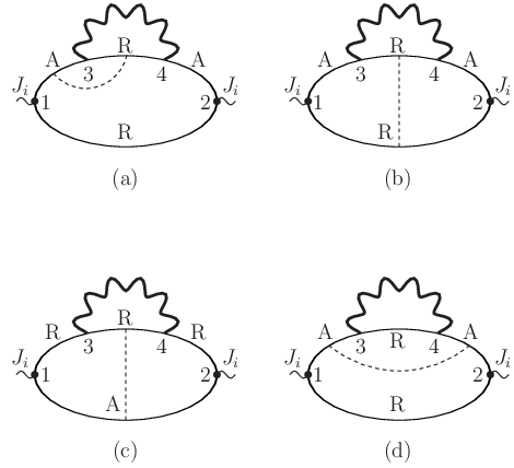
where is the Green’s function for non-interacting electrons in the presence of a random potential (i.e., before disorder average), and . The corresponding diagrams are shown in Fig. (1). The third step is to perform the disorder average which restores translation invariance. The disorder averaged electron Green’s function is given by
| (6) |
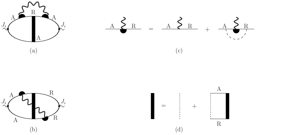
Here is the linearized electron dispersion as measured from the Fermi energy. The diagrams which contribute in the ballistic regime are shown in Figs. (1, 2), while those that are important in the diffusive regime are shown in Fig. (3). In these diagrams the electron propagator is denoted by a solid line, the propagator for the spin fluctuations by a wavy line, and an explicit impurity scattering (in contrast with the implicit ones which give elastic scattering lifetime to the electrons in Eq. (6)), which gives a factor of , by a dashed line.
The interaction correction to conductivity in the triplet channel can be written as zna
| (7) | |||||
where is the advanced bosonic propagator given by Eqs. (2) and (4), and is the fermionic part in the diagrams shown in Figs. (1, 2, 3) in dimensions two and three respectively. In the ballistic regime , and therefore diagrams with more than one explicit impurity scattering are sub-leading. The limiting form of in this regime is given by the leading term in from the sum of the diagrams given by Figs. (1, 2). The details of this evaluation is given in Appendix A. This approximation is equivalent to an expansion in near the QCP, and in for (i.e., in the FL regime). In this regime , and in two dimensions we get
| (8) |
where
| (9) |
while in three dimensions we get
| (10) |
where
| (11) |
In the diffusive regime , and multiple impurity scattering needs to be taken into account. altshuler The leading contribution is given by the diagrams in Fig. (3), whose evaluation is discussed in Appendix A. In this limit the kinematics of the electrons is governed by the diffusion pole, and we get , where
| (12) |
in dimensions .
III Results in two dimensions
From Eq. (7) the correction to conductivity in the triplet channel is
where is given by Eqs. (2) and (4) in the ballistic and diffusive regimes respectively, and by Eqs. (8) and (12) respectively.
III.1 Ballistic Regime
The ballistic regime is defined by for , by for , and by for . In this limit there are three crossover regimes (regions I-III in Fig. (4)).

Regime I. In order to calculate the leading behaviour in this regime one can set in Eq. (2), which gives the momentum scale . This is the typical momentum transferred by the spin fluctuations to the electrons during elastic scattering at temperature . The high- cut-off of this regime is , below which (in other words , where is the typical momentum of the fermionic excitations). As a result, the frequency dependence of in Eq. (8) can be ignored, giving . With these approximations we get
The last frequency integral is ultraviolet divergent for which we introduce a cut-off at . We get,
| (13) |
where
In Eq. (13), and in subsequent evaluations, we ignore a temperature independent contribution which renormalizes the residual conductivity. At finite the regime ends when , which gives the crossover temperature scale . For the effect of finite cannot be neglected.
The result in Eq. (13) can also be simply understood from the following scaling argument. The correction to the transport scattering rate can be estimated as , where is the self-energy of the electrons due to interaction with the spin fluctuations, and is the average time scale of the interaction. In this estimate is the quasiparticle scattering rate, which is renormalized by the factor in order to obtain a transport rate. Using the uncertainty principle we estimate , where is the typical momentum transferred during scattering between the electrons and the spin fluctuations. Near the QCP, , and scaling , we obtain the -dependence in Eq. (13).
Regime II. In this regime we identify two situations. (i) First, for , the approximate form of is given by dropping the term in Eq. (2), giving . The typical scale of momentum transferred during scattering is given by . Since in this sub-regime, the - dependence of can be ignored giving . We get
(ii) Second, for , the typical momentum scale is given by . In this sub-regime the Landau damping term in is order , and so it can be ignored giving (the situation is non quasi-static since , however the Landau damping term, whose universal form in Eq. (2) is correct only in the quasi-static limit, becomes unimportant for leading behaviour). We retain the full -dependence of given by Eq. (8), and we get
i.e., the same result as in sub-regime (i). For both the sub-regimes the triplet channel contribution to conductivity is
| (14) |
which is the result obtained in Ref. zna. The high- cut-off of sub-regime (ii) is given by , above which the term in cannot be neglected since .
Regime III. This is the high temperature regime of the theory where the typical momentum scale is . For , the damping term in the spin fluctuation propagator can be neglected since . For , the mass of the spin fluctuations can be neglected since . Thus, in this regime we get . Since
the leading order contribution to cancel out, and from sub-leading terms. In this regime the temperature dependence of conductivity is dominated by the contribution from the singlet channel (or by inelastic processes, if the electron system is on a lattice).
III.2 Diffusive Regime
Regime IV. Setting we get , which gives a possible momentum scale where . From the fermionic part given by Eq. (12), we get a second momentum scale . It can be shown that in this regime , which implies that the -dependence of can be ignored for the leading result, giving . With this approximation the resulting momentum integral is infrared divergent, which is cut-off by the ignored momentum scale . Using
we get
| (15) |
For finite this regimes exists for . Below the effect of finite cannot be neglected. This regime has been discussed previously in the context of metamagnetic QCP, kim and also in the context of fermionic gauge field models. mirlin; khveshchenko Note that our result gives a metallic sign to the -dependence of conductivity.
Regime V. In this regime the term in can be dropped, giving . This provides a new bosonic momentum scale . As in Regime II, two sub-regimes can be identified. (i) For we get , which implies that the -dependence of can be dropped, giving . Using as an infrared cut-off to the resulting momentum integral we get to leading order,
(ii) For we get . This implies that , while the full -dependence of has to be retained. We get
Combining the results of the two sub-regimes we get,
| (16) |
where for , and for . This is the famous Altshuler-Aronov correction to the conductivity for the triplet channel in the diffusive regime of good metals. altshuler
IV Results in Three Dimensions
From Eq. (7) we get,
where is given by Eqs. (10) and (12) in the ballistic and diffusive regimes respectively. As in , there are five different crossover regimes (I—V in Fig. (5)) for the leading temperature dependence of the correction to conductivity. The scale of the typical momentum transferred by the spin fluctuations to the conduction electrons during elastic scattering in each of these regimes remain the same as in . Consequently, the crossover lines delineating the five regimes also remain the same as in .
IV.1 Ballistic Regime
Regime I. Setting we get , and the typical momentum scale is , so that the -dependence of can be dropped giving . For the momentum integral we get
The leading temperature dependence of the correction to conductivity is given by
| (17) |
where
As in the case of , the result in Eq. (17) can be estimated from . Since , and , with and , we get the exponent of the temperature dependence in Eq. (17).

Regime II. As in , two situations can be identified in this regime. (i) For , , which gives the momentum scale . The -dependence of can be dropped, and from the momentum integral (which is ultraviolet divergent, and is cut-off at ) we get
(ii) For we have , and the typical momentum scale is . Keeping the full -dependence of we get,
After the -integral we get
| (18) |
where and for , and for .
Regime III. In the high- regime of the theory , and the typical momentum scale is . Keeping the full -dependence of we get
where . After the frequency integral we get,
| (19) |
IV.2 Diffusive Regime
Regime IV. Setting we get , which gives the typical momentum scale , where . Ignoring the -dependence of we have . From the momentum integral we get
The -integral gives
| (20) |
where
We note that the result given by Eq. (IV.2) is different from the result obtained in Refs. prl85 and belitz2. This is because in the latter the spin fluctuation propagator is dressed by the non-analytic term proportional to (which is sub-leading in our model). It is easy to see from a simple power counting argument that the exponent 1/3 is obtained by replacing the analytic term by a term.
Regime V. (i) For we have , , and is the typical momentum scale. The momentum integral gives
(ii) For , , and the typical momentum scale is . Keeping the -dependence of we get
After the frequency integral we get
| (21) |
where
and for , and for .
V Conclusion
To conclude, we have calculated the temperature dependence of the conductivity due to interaction correction for a disordered itinerant electron system close to a ferromagnetic quantum critical point in dimensions two and three. With an appropriate choice of parameters , where is the parameter associated with the Landau damping of the spin fluctuations and is the dimensionless coupling between the conduction electrons and the spin fluctuations, we are able to perform controlled calculations over the entire - plane, where is the mass of the spin fluctuations. Near the quantum critical point, the crossover between diffusive and ballistic regimes of transport occurs at a temperature which is few orders of magnitude smaller than the crossover temperature which is expected in the case of a good metal (sufficiently far away from any phase instability). The ballistic-diffusive crossover is determined by the temperature at which the typical length travelled by an electron during an electron-electron scattering event becomes comparable with the mean free path . Using uncertainty principle, this length can be estimated as , where is the momentum transferred by the spin fluctuation to the electron. In the quantum critical regime typical scales as which gives the crossover temperature (after scaling ). Away from the quantum critical regime, typical scales as , which gives the usual crossover scale for a good metal. In the ballistic regime near the quantum critical point (regime I in Figs. (4) and (5)), we obtained , which can be understood from the following scaling argument. In the ballistic limit the correction to the transport scattering rate due to electron-electron interaction can be estimated as , where is the average time scale of the interaction. This can be understood as the renormalization of the quasiparticle scattering rate by the factor in order to obtain a transport rate. Using the uncertainty principle, we estimate , where in the quantum critical regime. Now, since and , we get the temperature dependence of the conductivity. In the diffusive regime near the quantum critical point (regime IV in Figs. (4) and (5)) we found in and in . Moving out of the quantum critical regime we recovered the usual results for Fermi liquids (regimes II and V).
Acknowledgements.
This work was supported by the U. S. Dept. of Energy, Office of Science, under Contract No. DE-AC02-06CH11357. The author is very thankful to C. Pépin, D. L. Maslov, B. N. Narozhny, I. S. Beloborodov, J. Rech and A. Melikyan for insightful discussions.Appendix A
In this appendix we give the details of the calculation of the fermionic component in Eq. (7) in the ballistic and the diffusive limits.
A.1 Ballistic Regime
In this regime the leading contribution to the conductivity bubble is due to the diagrams shown in Figs. (1) and (2) (with the solid lines representing disorder averaged electron Green’s functions), i.e., those without any explicit impurity scattering, and those with one explicit impurity scattering respectively.
A.1.1
We begin by calculating the diagrams in Fig. (1). Note that diagrams (c), (d) and (e) have numerical pre-factors -1, -1, and 2 respectively (see their corresponding expressions in Eq. (5)). As an example we calculate the diagram in Fig. (1(a)). This is given by
| (22) | |||||
where refer to disorder averaged electron Green’s functions in Eq. (6), and is the volume of the system. The momentum sum in the above Eq. is dominated by the contribution near the Fermi surface where the spectrum can be linearized, and (assuming an isotropic system). Replacing
where , the energy integral is given by
which can be solved by contour integration. The diagonal component of the tensor is given by
where , and
| (23) |
The remaining diagrams (b) — (e) in Fig. (1) can be evaluated similarly, giving respectively
| (24) | |||||
| (25) | |||||
| (26) | |||||
| (27) |
The leading behaviour in the ballistic limit is given by the first non-vanishing term of the expansion of the fermionic part in the parameter . We note that and have terms of which cancel, which implies that the leading behaviour is due to terms of . As a result contributions from and are sub-leading, and can be ignored. The remaining contributions are generated by introducing one explicit impurity line (represented by dashed line), which gives a factor of , in diagrams (a) and (b) in Fig. (1). These second set of contributions are shown in Fig. (2) (note that the diagram in Fig. (2(a)) has a factor of due to symmetry). The contribution from these diagrams are respectively given by
| (28) | |||||
| (29) | |||||
| (30) |
Adding all the terms inside the square brackets in , and considering only the leading term in we get Eqs. (8) and (9).
A.1.2
In the logic of the evaluation of the fermionic part is the same as in the two-dimensional case. The only difference is in the evaluation of angular integrals during Fermi surface averages, since in
where . For example, the diagram in Fig. (1(a)) is now given by
| (31) | |||||
where
| (32) |
The remaining diagrams are given by
| (33) | |||||
| (34) | |||||
| (35) | |||||
| (36) | |||||
| (37) |
We do not give results for and since they are sub-leading. Adding all the leading terms inside the square brackets in the expressions for , we get Eqs. (10) and (11).
A.2 Diffusive Regime
In this regime multiple impurity scattering is important. Consequently, the interaction vertex is dressed by a ladder of impurity lines (Fig. 3(c)). Similarly, a single impurity line is replaced by the same ladder (Fig. 3(d)). The leading contributions to the conductivity are due to the diagrams shown in Figs. (3(a)) and (3(b)). Note that diagram (3(b)) has a symmetry factor of .
A.2.1
In this regime , so that we get , where is the diffusion constant. The dressed interaction vertex is given by
evaluating which gives
| (38) |
Similarly, the ladder of impurity lines is given by
| (39) |
The diagram in Fig. (3(a)) is given by
where
where is a unit vector. Replacing by for diagonal components of the conductivity tensor, and using the approximate forms for and we get,
| (40) |
Similarly, the diagram in Fig. (3(b)) is given by
| (41) |
Adding the terms in the square brackets in and we get in Eq. (12).

A.2.2
Expanding in the small parameters we get , with the diffusion constant in three dimensions given by . It is easy to check that the approximate expressions for and are the same as those in two dimensions (with the appropriate re-definition of the diffusion constant). Next, we get
Using the approximate forms of , and we get
| (42) | |||||
| (43) |
Adding the terms in the square brackets in the above two Eqs. we get in Eq. (12).
Appendix B
In this appendix we discuss the effect of adding a vertex correction to the spin-fermion coupling in the conductivity calculation for the ballistic limit of the quantum critical regime. Using Eq. (3) we show that, even though the spin fluctuation is massless, a vertex correction gives rise to sub-leading contribution to the temperature dependence of conductivity. We demonstrate this explicitly for the diagram shown in Fig. (6), which is a typical example. The behaviour of other vertex correction diagrams are expected to be similar.
B.1
In order to facilitate the discussion we will first evaluate the diagram shown in Fig. (2(a)) in Matsubara frequency, and then compare it with the evaluation of the corresponding vertex diagram (Fig. (6)). Writing the contribution of the former to the current-current correlator as we get,
where is fermionic Matsubara frequency, and are bosonic Matsubara frequencies, and is the disorder averaged electron Green’s function in Matsubara frequency. The factor in front is due to the symmetry of the diagram. The integral in the above expression is non-zero only if and have opposite signs. Next, for the integral the dominant contribution occurs when and have opposite signs. For , the leading term in is given by,
| (44) | |||||

After performing the sum, and taking the limit of static conductivity, we get Eq. (7) with . This is the contribution to conductivity from the diagram in Fig. (2(a)) [see expression for in Appendix A]. The evaluation of the vertex diagram (Fig. (6)) is analogous. Writing its contribution to the current-current correlator as we get,
As in the case of , the leading contribution comes from , , and . Taking into account only the leading dependence in we get (for ),
Here
at zero temperature. rech0 Using the above expression and performing the angle integration we finally get,
| (45) | |||||
Comparing the expressions for and we get that in regime I, where , the vertex correction also yields , but with a pre-factor which is parametrically small in . In the high temperature regime of the theory (regime III), where , the vertex correction is small by .
B.2

In three dimensions the estimation of the vertex diagram is entirely analogous to the case. The contribution to the current-current correlator from the diagram shown in Fig. (2(a)) is given by
| (46) | |||||
On the other hand, the corresponding contribution from the vertex diagram of Fig. (6) is given by
| (47) | |||||
Comparing the expressions for and we get that in regime I, where , the vertex correction is parametrically small in . In the high temperature regime of the theory (regime III), where , the vertex correction is small in .
Appendix C
In this appendix we calculate the leading self-energy correction of the electron propagator in the diffusive limit of the quantum critical regime. This is given by the diagrams shown in Fig. (7). It is to be noted that there are four other contributions which are important for the self-energy away from the quantum critical regime where FL results are recovered (i.e., in Regime V of Figs. (4) and (5)), adamov but which are sub-leading in the quantum critical regime. Using Eq. (3) we show that the self-energy correction is much smaller than the elastic scattering rate , and therefore such a correction can be omitted in a perturbative calculation. Furthermore, we argue that the terms which are second order in the spin-fermion coupling are sub-leading in the diffusive quantum critical regime due to Eq. (3). We demonstrate this explicitly for the diagram shown in Fig. (8). The behaviour of the other second order terms are expected to be similar or smaller.
C.1
First we evaluate the self-energies given by Fig. (7). Denoting the diagram (a) as , we have
where the prime in the frequency summation indicates the condition that , and where in the diffusive limit. We evaluate the above expression at the pole of the electron Green’s function, i.e., at such that . adamov This gives
In the above the leading term in an expansion in is divergent, but this divergence is canceled by the diagram (b) in Fig. (7). The latter contribution, which is momentum independent is given by,
In the diffusive limit of the quantum critical regime we have , using which we get
| (48) |
to the lowest order in . In the above we ignored a constant part coming from the ultraviolet cut-off. Scaling , and using Eq. (3) we conclude that for , . Thus, the self-energy correction can be ignored for the evaluation of the leading temperature dependence of the conductivity.
Next, we evaluate the contribution to the current-current correlator from the diagram shown in Fig. (8). For this we define
and . Then the current-current correlator can be written as
In the above the restrictions on the frequency summations are such that, for , we have , , and . For the purpose of an estimation, we perform the -summation without restriction, and we get
| (49) | |||||
By comparing with a typical contribution to the current-current correlator at first order in , we conclude that the contribution from the diagram shown in Fig. (8) is smaller by a factor of .
C.2
In three dimensions the calculations are entirely analogous to the case. For the self-energy given by Fig. (7) we get
| (50) |
which is smaller than for , and therefore can be neglected. Next, we estimate the contribution to the current-current correlator from the diagram in Fig. (8), and we find that it is smaller than those that are first order in by a factor of .
References
- (1) B. L. Altshuler, and A. G. Aronov, Electron-Electron Interactions in Disordered Systems, edited by A. L. Efros and M. Pollak (North-Holland, Amsterdam, 1985), and references therein.
- (2) I. L. Aleiner, B. L. Altshuler, and M. E. Gershenson, Waves Random Media 9, 201 (1999).
- (3) G. Zala, B. N. Narozhny, and I. L. Aleiner, Phys. Rev. B 64, 214204 (2001).
- (4) for a review see e.g., G. R. Stewart, Rev. Mod. Phys. 73, 797 (2001).
- (5) I. Paul, C. Pépin, B. N. Narozhny, and D. L. Maslov, Phys. Rev. Lett. 95, 017206 (2005).
- (6) Y. B. Kim, and A. J. Millis, Phys. Rev. B 67, 085102 (2003).
- (7) D. Belitz, T. R. Kirkpatrick, R. Narayanan, and T. Vojta, Phys. Rev. Lett. 85, 4602 (2000).
- (8) D. Belitz, T. R. Kirkpatrick, M. T. Mercaldo, and S. L. Sessions, Phys. Rev. B 63, 174428 (2001).
- (9) A. Rosch, Phys. Rev. Lett. 82, 4280 (1999).
- (10) C. Pfleiderer, and A. D. Huxley, Phys. Rev. Lett. 89, 147005 (2002).
- (11) M. Uhlarz, C. Pfleiderer, and S. M. Hayden, Phys. Rev. Lett. 93, 256404 (2004).
- (12) S. A. Grigera, R. S. Perry, A. J. Schofield, M. Chiao, S. R. Julian, G. G. Lonzarich, S. I. Ikeda, Y. Maeno, A. J. Millis, and A. P. Mackenzie, Science 294, 329 (2001).
- (13) A. J. Schofield, A. J. Millis, S. A. Grigera, and G. G. Lonzarich, in Springer Lecture Notes in Physics, 603, 271 (2002).
- (14) S. A. Grigera, P. Gegenwart, R. A. Borzi, F. Weickert, A. J. Schofield, R. S. Perry, T. Tayama, T. Sakakibara, Y. Maeno, A. G. Green, and A. P. Mackenzie, Science 306, 1154 (2004).
- (15) D. A. Sokolov, M. C. Aronson, W. Gannon, and Z. Fisk, Phys. Rev. Lett. 96, 116404 (2006).
- (16) P. A. Lee, and T. V. Ramakrishnan, Rev. Mod. Phys. 57, 287 (1985).
- (17) A. D. Mirlin, and P. Wölfle, Phys. Rev. B 55, 5141 (1997).
- (18) D. V. Khveshchenko, Phys. Rev. Lett. 77, 362 (1996).
- (19) V. M. Galitski, Phys. Rev. B 72, 214201 (2005).
- (20) J. A. Hertz, Phys. Rev. B 14, 1165 (1976); T. Moriya, Spin Fluctuations in Itinerant Electron Magnetism, (Springer-Verlag, Berlin, New York, 1985); A. J. Millis, Phys. Rev. B 48, 7183 (1993).
- (21) D. Belitz, T. R. Kirkpatrick, and T. Vojta, Phys. Rev. B 55, 9452 (1997).
- (22) Ar. Abanov, and A. V. Chubukov, Phys. Rev. Lett. 93, 255702 (2004).
- (23) D. Belitz, T. R. Kirkpatrick, and T. Vojta, Rev. Mod. Phys. 77, 579 (2005).
- (24) Ar. Abanov, A. V. Chubukov, and J. Schmalian, Adv. Phys. 52, 119 (2003).
- (25) A. A. Abrikosov, L. P. Gorkov, and I. E. Dzyaloshinski, Methods of Quantum Field Theory in Statistical Physics, (Dover Publications Inc., New York, 1963).
- (26) A. V. Chubukov, and D. L. Maslov, Phys. Rev. B 68, 155113 (2003); G. Y. Chitov, and A. J. Millis, Phys. Rev. Lett. 86, 5337 (2001).
- (27) A. V. Chubukov, C. Pépin, and J. Rech, Phys. Rev. Lett. 92, 147003 (2004).
- (28) T. R. Kirkpatrick, and D. Belitz, Phys. Rev. B 53, 14364 (1996).
- (29) A. Kamenev, and Y. Oreg, Phys. Rev. B 52, 7516 (1995).
- (30) J. Rech, C. Pépin, and A. V. Chubukov, Phys. Rev. B 74, 195126 (2006).
- (31) Y. Adamov, I. V. Gornyi, and A. D. Mirlin, Phys. Rev. B 73, 045426 (2006).