The Minimally Tuned Minimal Supersymmetric Standard Modelrouven@physics.rutgers.edujffor27@physics.rutgers.edu
Abstract
The regions in the Minimal Supersymmetric Standard Model with the minimal amount of fine-tuning of electroweak symmetry breaking are presented for general messenger scale. No a priori relations among the soft supersymmetry breaking parameters are assumed and fine-tuning is minimized with respect to all the important parameters which affect electroweak symmetry breaking. The superpartner spectra in the minimally tuned region of parameter space are quite distinctive with large stop mixing at the low scale and negative squark soft masses at the high scale. The minimal amount of tuning increases enormously for a Higgs mass beyond roughly 120 GeV.
1 Introduction
The Minimal Supersymmetric Standard Model (MSSM) is a well-motivated candidate for physics beyond the Standard Model (SM). The gauge couplings within the MSSM unify to within a few percent at the grand unified theory (GUT) scale, GeV, and the lightest supersymmetric particle is a good dark matter candidate provided that R-parity is conserved. Supersymmetry (SUSY) can also naturally stabilize the hierarchy between the electroweak (EW) and the GUT or Planck scale. It does this by providing a radiative mechanism for electroweak symmetry breaking (EWSB) where large quantum fluctuations of the scalar top squarks due to the large Yukawa coupling destabilize the origin of the Higgs potential. In much of the MSSM parameter space this quite naturally leads to the right EWSB scale, as long as the soft SUSY breaking parameters lie near it.
The absence of any direct experimental evidence from collider searches for the MSSM scalar particles and the Higgs boson has, however, ruled out significant regions in the MSSM parameter space. Indirect evidence from EW precision measurements and searches for flavor changing neutral currents, CP violating effects and rare decays has not been forthcoming either, providing additional severe constraints. As a result the soft SUSY breaking parameters must lie well above the EW scale in order to satisfy the experimental constraints, especially the constraints on the Higgs mass from the results of the CERN LEP collider ( GeV [1]).
Soft SUSY breaking parameters well above the EW scale reintroduce a small hierarchy and require some fine-tuning (FT) among the SUSY parameters in order to obtain EWSB [2]-[22]. This is usually referred to as the supersymmetric little hierarchy problem.
Different choices for the soft SUSY breaking parameters lead to different amounts of FT. This paper presents the minimally tuned MSSM (or MTMSSM), i.e. the MSSM parameter region that has the least model-independent FT of EWSB. Model-independent means that no relations are assumed between the soft SUSY breaking parameters at the scale at which they are generated (which will be referred to as the messenger scale). Rather, each of them is taken to be an independent parameter which is free at the messenger scale, and which therefore can contribute to the total FT of the EWSB scale. The messenger scale itself is varied between 2 TeV and and the effect of this on the minimal FT is discussed (see also [14, 15]).
In Section 2, EWSB in the MSSM will be reviewed. Section 3 discusses the tuning measure used in this paper. The parameters taken to contribute to the tuning are , , the gaugino masses , and , the stop soft masses and , and the stop soft trilinear coupling .
Section 4 contains some of the main results. The low- and high-scale MSSM spectrum which leads to the least model-independent FT is found. This is done for various messenger scales by numerically minimizing the FT expression subject to constraints on the Higgs, stop, and gaugino masses. The results are then motivated analytically. The least FT is found to be about 5 if the messenger scale coincides with the GUT scale. An important feature of the least FT region is negative stop soft masses at the messenger scale (first pointed out in [19]). Even for messenger scales as low as 2 TeV, the stop soft masses are tachyonic at the messenger scale (threshold effects in the RG-running were neglected throughout). This does not lead to any problems with charge and/or color breaking minima. Another feature of the least FT region is that the trilinear stop soft coupling, , is negative and lies near “natural” maximal mixing, i.e. , where is the average of the two stop soft masses. This value for maximizes the radiative corrections to . The large stop mixing leads to a sizeable splitting between the two stop mass eigenstates. Moreover, the gluino mass, , is much smaller than the wino mass, , at the high scale. The wino mass, in turn, is much smaller than the bino mass . Phenomenological consequences of the low-scale spectrum are briefly summarized.
Section 5 contains the rest of the main results of the paper. The FT is minimized as a function of the lower bound on the Higgs mass (with the messenger scale set to ). Although the numerical minimization procedure contains the dominant one-loop expression for as a constraint, the resulting least FT spectra are used to calculate more accurately with the program [23, 24, 25, 26, 27]. The result is a plot of the minimal FT as a function of . There are several striking features of this plot. First of all, for larger than a certain value, the FT increases very rapidly. Secondly, around this , the value of in the least FT region makes a sudden transition from lying near to lying near . The third striking feature is that this value of is surprisingly low. The precise value is only slightly dependent on the parameters in the Higgs sector and can be taken to lie around 120 GeV. The upshot of this analysis is that although the MSSM right now is already fine-tuned at least at about the level (if the messenger scale equals the GUT scale), there is not much room left for the Higgs mass to increase before the FT becomes exponentially worse.
Section 6 contains a summary of the results and the conclusions. Appendix A reviews the semi-numerical solutions of the MSSM one-loop renormalization - group (RG) equations. These are used to calculate the expression for the FT employed in this paper. Appendix B contains a list of expressions for the FT with respect to various parameters.
2 Electroweak Symmetry Breaking
In the Higgs decoupling limit of the MSSM, the lower bound on the mass of the lighter CP-even Higgs mass eigenstate coincides with the 114.4 GeV bound on the mass of the SM Higgs boson [1]. The mass of may be approximated by
| (1) |
which, in addition to the tree-level Higgs mass, includes the dominant one-loop quantum corrections coming from top and stop loops [28, 29, 30, 31, 32, 33]. Here is the top mass, is the arithmetic mean of the two squared stop masses and GeV where is the gauge coupling and is the mass of the -boson. Furthermore, equation (1) assumes . The stop mixing parameter is given by ( for large ), where denotes the stop soft trilinear coupling and is the supersymmetric Higgsino mass parameter. The first term in equation (1) is the tree-level contribution to the Higgs mass. The first term in square brackets comes from renormalization group running of the Higgs quartic coupling below the stop mass scale and vanishes in the limit of exact supersymmetry. It grows logarithmically with the stop mass. The second term in square brackets is only present for non-zero stop mixing and comes from a finite threshold correction to the Higgs quartic coupling at the stop mass scale. It is independent of the stop mass for fixed , and grows as for small .
Equation (1) implies a combination of three things which are required to satisfy the bound on , namely a large tree-level contribution, large stop masses and large stop mixing. A large tree-level contribution to requires to be at least of a moderate size (). Although the stop masses must be rather large, their lower bound is very sensitive to the size of the stop mixing, with larger mixing allowing for much smaller stop masses (see [34] for a recent study on this). The reason for this sensitive dependence is due to the Higgs mass depending logarithmically on the stop masses in contrast to the polynomial dependence on the stop mixing.
The soft masses are not only directly constrained from the LEP Higgs bounds but also indirectly by constraints on flavor changing neutral currents, electroweak precision measurements and CP-violation. Besides these, however, the Higgs sector parameters are also constrained by requiring that the electroweak symmetry is broken. This leads to the following two tree-level relations at the low scale
| (2) |
| (3) |
where is the CP-odd Higgs mass, and is determined from the ratio of the two vacuum expectation values and as . The masses , and are the three soft mass parameters in the MSSM Higgs sector. For a given value of , may be eliminated in favor of with equation (2). Equation (3) gives an expression for in terms of the supersymmetric mass parameter and the soft masses and . Since should be sizeable, the contribution from to the expression for may be neglected and (3) simplifies to
| (4) |
Close to the Higgs decoupling limit, is relatively large. However, since to avoid large cancellations, may not be too large, otherwise would also be sizeable and equation (4) would break down (unless the value of is increased accordingly). By choosing and GeV in the numerical analysis throughout, equation (4) holds to a very good approximation.
Equation (4) holds at tree-level, and although quantum corrections may add (10 GeV) to the right hand side of (4), this has negligible impact on the amount of fine-tuning to be discussed below.
The parameters and in equation (4) are evaluated at the scale . Since the fine-tuning of EWSB is a measure of the sensitivity of some low-scale EWSB parameter (usually taken to be ) to a change in high-scale input parameters, and need to be evolved to a high scale using their RG equations. Under RG running many of the soft parameters mix, and as a result of this mixing, the expression for in terms of parameters that are evaluated at the messenger scale differs significantly from the simple form given in (4). The RG-equations may be integrated (see Appendix A) and the expression for may generically be written as [35, 36]
| (5) |
For moderate and not too large values of with an appropriate , the simplified expression for is applicable (equation (4)) and contributions from the bottom/sbottom and tau/stau sectors may still be neglected. The most important parameters appearing in (5) then are , , the gaugino masses , and , the stop soft masses and , and the stop soft trilinear coupling . The coefficients depend on and the messenger scale . The most important coefficients are shown in Figure 1 for as a function of .

At the scale , the coefficients of and are while the coefficients of the other soft parameters are zero in agreement with equation (4). Since is a supersymmetric parameter, it gets renormalized multiplicatively and its RG evolution does not give rise to soft parameters (see equation (45)). Figure 1 shows that the coefficient of does not vary much and remains close to all the way up to the GUT scale. The RG evolution of to higher messenger scales, however, generates non-zero coefficients for the other soft parameters. The -function of ,
| (6) |
depends on the stop sector parameters , the wino and bino masses and , and , which thus get generated immediately under RG evolution. The coefficients of and especially and in (6) are small and lead to small coefficients in the expression for (5). Although does not explicitly depend on the gluino mass, a non-zero coefficient for is generated indirectly since the stop sector -functions depend on . Moreover, appears with a large coefficient in these -functions, and thus the coefficient of in equation (5) dominates after a few decades of RG evolution. For example, at a messenger scale of GeV, the expression for (for = 10) is
| (7) | |||||
where the hatted parameters on the right-hand side are all evaluated at . This expression may be used to calculate the FT as discussed next.
3 The Tuning Measure
A variety of tuning measures have been used in the literature (a list of references has been provided in the Introduction). Since the concept of fine-tuning (FT) is inherently subjective, there is no absolute definition of a FT measure. The most common definition of the sensitivity of an observable on a parameter , denoted by , is given by [2, 3]
| (8) |
thus measures the percentage variation of the observable under a percentage variation of the parameter. A large value of signifies that a small change in the parameter leads to a large change in the observable, and suggests that the observable is fine-tuned with respect to that parameter. Assuming that the individual are uncorrelated, they may be combined to form the FT measure
| (9) |
Of interest in this paper is to quantify the sensitivity of EWSB in the MSSM on (soft) supersymmetric parameters at the messenger scale . To this end, the observable to consider is as a function of the supersymmetric Higgsino mass squared and the soft supersymmetry breaking parameters, collectively denoted by (in the FT measure, all parameters are taken to have mass dimension two). The sensitivity of with respect to each parameter may be calculated as in (8) with , and the total FT of on parameters evaluated at the messenger scale may be quantified by
| (10) |
may be interpreted as the length of a “fine-tuning vector” with components . This fine-tuning vector is formally a vector field defined by the gradient of the scalar field , a function of , along surfaces of constant .
There are several possible drawbacks to this FT measure, see for example [22, 37]. One of these is that the individual are assumed to be uncorrelated. Within a given model of supersymmetry breaking, there may be relations among the parameters at the messenger scale. This would imply that the FT vector is projected onto a subspace, and the resulting FT is necessarily less. In other words, the tuning of one parameter is correlated with the tuning of another, so that the total FT should be less than that given by (10). Moreover, within a given model the values of the parameters at the messenger scale may be restricted to certain ranges, whereas (10) assumes that all values are equally likely. However, no model for supersymmetry breaking will be assumed here. Instead, the minimal FT will be found as a function of the messenger scale assuming no relations or restrictions among the high-scale input parameters. For this “model-independent” tuning it is satisfactory to use the FT measure (10).
Note that to find the tuning of a model, one should in principle consider the tuning of all observables, since the absence of tuning in one observable does not necessarily imply it is small in others, see e.g. [17]. In this paper, however, only the tuning of EWSB will be considered.
Finally, note that the FT with respect to a single parameter is by definition (8) zero if that parameter happens to be zero at the messenger scale. An extreme version of this is found in the no-scale model [38], where all scalar soft masses are much smaller than the gaugino masses at the high scale. Setting them to zero, and using (8) and (10) the FT could be expected to be small. However, it may be shown that this does not minimize the FT, since and need to be quite large at the high scale to satisfy all the low-energy experimental bounds (see [13]). In the results presented in this paper, no parameter is found to be zero at the high scale.
4 Minimal Model Independent Tuning
In this section the minimal model independent tuning will be found as a function of the messenger scale.
4.1 Discussion of Minimization Procedure and Constraints
The FT given by equation (10) is written in terms of parameters evaluated at the messenger scale. In order to find the minimal FT (MFT) for a given messenger scale that is consistent with low-energy experimental constraints, it is easiest to rewrite the FT expression in terms of parameters that are evaluated at the low scale. This can be done by expressing each high-scale parameter in terms of low-scale parameters, see Appendix A. Once the FT is written in terms of low-scale parameters, may be eliminated by using equation (4) (neglecting contributions from ).
The low-energy constraints considered in this paper include bounds on the (physical) sparticle masses, on the gaugino masses, and on the Higgs mass11 1 Constraints from measurements of or the electroweak - and -parameter do not significantly affect the results presented below, since an experimentally consistent value can be obtained by only small adjustments (if at all necessary) in the least fine-tuned parameters - see also [34].. The top quark mass is set to the central value of the latest Tevatron mass measurement of 170.9 1.8 GeV [39]. The physical stop masses are required to be at least 100 GeV which is illustrative of the actual, slightly model dependent, lower bound obtained from the Tevatron [40]. It is found that the region of MFT does not quite saturate this bound, although a slightly larger value for would allow the lighter stop to be as low as 100 GeV. The gaugino masses and , as well as , are taken to have a lower bound of 100 GeV. The gluino mass is found to be never smaller than 335 GeV in the numerical results presented in this section, and this does not generically violate any experimental bounds.
The most important constraint is the Higgs mass bound of 114.4 GeV (valid in the decoupling limit), since it turns out that this bound is always saturated when minimizing the FT. In the numerical results presented in this paper, the Higgs mass is calculated using the formulas found in [41] (see also [28, 29, 30, 31, 32, 42]). These formulas include the one-loop corrections coming from the top/stop sector and are simple enough to be used as constraints in the FT minimization (but note that the sign convention used for is that of [43]). A running top mass , evaluated in the -scheme, is used to capture some of the leading two-loop contributions. Higher-order corrections to the Higgs mass still play a very important role, however, and more accurate Higgs masses may be obtained with the program . In order to take some of these higher-order corrections into account and thus obtain a more accurate estimate of the MFT, a lower bound for the Higgs mass of 121.5 GeV is used in the FT minimization, instead of the SM lower bound of 114.4 GeV. The typical low energy sparticle spectrum obtained in the analysis then leads to Higgs masses that satisfy the SM Higgs bound when calculated with (version 2.6.0, assuming real parameters).
Sequential Quadratic Programming (SQP) is used as a minimization algorithm. Given the FT function (10) written in terms of low scale parameters, as well as linear constraints on the gaugino masses and , non-linear constraints on the physical stop and Higgs masses, and an initial guess, SQP generates a less FT point until the minimum is found. Unlike other minimization algorithms, SQP can handle arbitrary constraints which is essential here due to the highly non-linear physical stop mass and Higgs mass constraints.
4.2 Numerical Results
Figure 2 shows a plot of the MFT as a function of the messenger scale . Shown are the individual contributions to the FT, with given by , , , , , or . The FT of and have been included as
| (11) |
The (top) black line shows the total FT as defined by (10).

From the plot it is clear that the MFT increases as a function of the messenger scale . This is expected since a higher messenger scale implies more RG running to the low scale so that small differences in high-scale input parameters are magnified. For , the total MFT is about 22, i.e. 4.5. (As an aside, for and , the MFT for a Higgs mass of 114 GeV is about 11, i.e. 9.) The largest contribution to the total minimal FT comes from and which are both comparable for all values of . The next most important contribution is that from . The contributions from , as well as and are less important and increase only slightly as a function of . The FT from is very small for all messenger scales while the contribution from is negligible for small and large but larger for intermediate messenger scales.
The large contribution from is mainly because it has the largest (in magnitude) coefficient in the expression for , at least for GeV, see Figure 1. The coefficients of the cross-terms , and are smaller (see Appendix B), but together still contribute about 40 of the FT with respect to for . The reason that the cross-term contributions are so large is that the MFT values of , , and are rather sizeable at the messenger scale when compared with (at least for GeV). This is depicted in Figure 3.

The FT of with respect to is also very large even though the coefficients of and the cross-terms , and in the expression for are rather small (for , about 50 of the FT comes from the cross-terms). This is again because , and are sizeable at . The contribution to the FT from is large for similar reasons.
The FT with respect to increases only slightly as a function of since the coefficient of in the expression for does not vary much, and since the high-scale value of increases only slightly as is increased. The contribution from is smaller than those from , and because the value of is comparatively small and also because there are no cross-terms in the FT expression that involve and other (large) soft parameters. Similar reasoning holds for the contributions from , and .
| -610 GeV | 305 GeV | 110 GeV | 475 GeV |
The low-energy spectrum that gives the MFT for a given messenger scale remains roughly unchanged as the messenger scale changes. The value of the stop soft trilinear coupling at the low scale is always about -610 GeV, with the two physical stop masses around 110 GeV and 475 GeV, respectively, see Table 1 and Figure 4. These values of the stop-sector parameters are essentially determined by the constraint on the Higgs mass and from the minimization of . The ratio is approximately -2, where , and . The MFT is thus found for the natural maximal-mixing scenario which approximately maximizes the radiative corrections to the Higgs sector for a given set of parameters and for negative [34, 44, 45, 46]. Small deviations of (and to a lesser extent and ) from its MFT value at the low scale lead to a very large increase in the FT, mainly from . This can be seen from (23), which shows that the largest coefficients in the expression for in terms of low-scale parameters all involve powers of . Note that for generic points in the still allowed parameter space, would give one of the largest contribution to the FT. To minimize the FT it is thus best to minimize which essentially determines the values of the stop-sector parameters (see the discussion in Section 4.3). The other contributions to the FT are then not at their minimum, but they are much smaller and less sensitive to variations in the parameters.

The low-scale values of the gaugino masses that give the MFT for a given messenger scale are shown in Figure 4. While the value of that gives the MFT is roughly the same for all , the values of and decrease for larger . Changing away from its MFT value does affect the FT but not excessively so, while a change in has a larger effect. The -parameter is always found to be less than 150 GeV for the MFT region at any messenger scale. Choosing it to be closer to 100 GeV instead has a negligible impact on the FT, and allows a neutralino to be the lightest SM superpartner (LSP), instead of the lighter stop, which is found to be the LSP in the numerical minimization procedure.
Negative may be expected to lead to less FT than positive because has a strongly attractive infrared quasi-fixed point near [47, 48]
| (12) |
(This relation is strictly valid only at the Pendleton-Ross quasi-fixed point for the top Yukawa [49], and neglecting and gauge interactions.) Because of this it is most natural for and to have opposite sign and be comparable in magnitude at low scales due to renormalization group evolution, see Figure 5. For positive and maximal-mixing in the stop-sector, would have to be an order of magnitude larger then at the messenger scale (see Figure 5) which would lead to a much more FT parameter region. The MFT region here does not satisfy (12) exactly, but instead at the low scale, for . In order to satisfy (12) exactly, would have to be larger (assuming remains fixed). This would increase the size of the stop masses under RG evolution as can be seen from their -functions, see (50) and (51), which would lead to increased FT.

The MTMSSM has negative soft squark squared masses at the messenger scale (see also [19]). This remains the case even if the messenger scale is very low and only on the order of a few TeV (for very low messenger scales, finite threshold corrections should really be included). Under RG-evolution the masses get driven positive very quickly within about a decade of running. It is the sizeable values of the gaugino masses that pull them up towards positive values. For smaller messenger scales the MFT region has a larger gluino mass, which drives the squark masses to positive values even faster while running towards the infrared. Equations (22) and (24) or (25) in Appendix A show that negative squarks at the messenger scale lead to more stop-mixing at the low scale, as was pointed out in [19]. Figure 6 shows the RG-trajectories of the MFT region if the messenger scale is =.
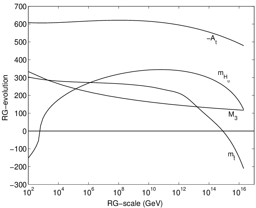
The presence of tachyonic squarks at the messenger scale [50, 51] and/or very large [52, 53] may lead to dangerous color and/or charge breaking (CCB) minima.
Very large may result in dangerous CCB minima around the EW scale. These CCB minima occur in the plane [54]. The condition that the EW minimum is the global minimum may be estimated by going along the D-flat direction = = and is given by [55]
| (13) |
Assuming instead that the EW minimum is only metastable but has a large enough lifetime gives the weaker constraint [55]
| (14) |
The MTMSSM easily satisfies the second condition, as well as satisfying the first condition. There are thus no dangerous CCB minima resulting from large .
Tachyonic stops at the messenger scale may result in an unbounded from below potential along D-flat directions involving the stop fields, as well as first and/or second generation squark fields or slepton fields. Loop corrections give rise to an effective potential which is not unbounded from below, but they generically introduce a CCB minimum with a vacuum expectation value (VEV) on the order of the messenger scale. The MTMSSM may thus have CCB minima with a VEV around the EW scale if the messenger scale is low, or CCB minima with a VEV large compared to the EW scale if the messenger scale is high. Since the EW minimum is metastable and long-lived for [56], it turns out that these CCB minima are not dangerous in the MTMSSM. Moreover, the MTMSSM does not determine the masses of the sleptons or first and second generation squarks since these do not play an important role in the FT. It is thus always possible to choose them in such a way to avoid CCB minima without changing the above FT results.
Finally, it is interesting to note that there are several near degenerate parameter subspaces along which the FT does not change much. The first and second generation particles and their superpartners do not contribute much to the FT because in equation (5) they appear only with a small coefficient. The parameter is also not very important for the same reason. A more interesting near degenerate subspace is that the FT is rather insensitive to changes in the difference of the two stop soft mass squared parameters at the low scale as long as their sum is kept fixed. This may be understood from the expression for , e.g. equation (7), in which only their sum appears (using the one-loop RG equations). However, even with only one-loop RG equations this degeneracy is not exact since small discrepancies appear in the FT measure from equations (24) and (25). Moreover, the difference in the two stop soft mass squared parameters appears in the calculation of the physical stop masses and this affects the size of the Higgs mass, which is the most crucial low-energy constraint when calculating the FT. The FT only starts to change by an order one number when GeV for .
4.3 Analytic Motivation for Numerical Results
The numerical results presented in section 4.2 may be motivated analytically. The discussion will for now assume , but generalizes to arbitrary with a few caveats discussed below.
In order to get a physical Higgs mass satisfying the experimental bound without generating large FT for the EWSB, it is natural to maximize the radiative corrections to . Due to the strongly attractive quasi-fixed point for , this is achieved for negative near (natural) maximal mixing (at least for not too large, see Section 5).
The most important contribution to the FT comes from since it has the largest coefficients, see Appendix B. Eliminating with the EWSB equation (7) and using the average stop soft mass squared gives
| (15) | |||||
It is possible to have cancelations among the various terms in this expression. also has large coefficients, but cancelations among its terms are impossible since is negative (see Appendix B).
Ignoring , cancelation of the largest terms in equation (15), i.e. the gluino term and the average stop soft mass squared term, decreases the FT by setting and leads to tachyonic squarks at the messenger scale [19]
| (16) |
Next, the four terms on the second line of equation (15) can cancel by taking
| (17) |
Assuming , this simplifies to . Furthermore, keeping only the most important terms, the natural maximal-mixing scenario implies
| (18) | |||||
which leads to , again assuming . It is now possible to compute the ratio of the soft trilinear coupling with the gluino mass at the EWSB scale,
| (19) |
These results agree well with the numerical results presented in section 4.2.
Note that a GUT scale model which predicts degenerate and negative squark and slepton soft masses at the GUT scale would need very large wino and bino masses in comparison to the gluino mass in order to drive the slepton soft masses to positive values under RG running to the EWSB scale [57]. This is due to the small coefficients of the bino and wino masses in the -functions of the slepton soft masses. It is interesting that the MFT region prefers the bino mass larger than the wino mass and, in turn, the wino mass larger than the gluino mass.
Although this cancelation pattern holds to a good approximation for higher messenger scales, does not exactly cancel as the messenger scale decreases. For lower messenger scales, becomes less tachyonic while increases, allowing the stop masses to be driven positive faster under RG running to the EWSB scale. Moreover, the coefficient of in the expression for (5) decreases significantly, as can be seen in Figure 1. Therefore the cancelation pattern in discussed above does not hold since the contribution decreases while the term gives a comparable contribution for all messenger scales (except for very small messenger scales). On the other hand, being a supersymmetric parameter, and its coefficient in equation (5) does not change much for different messenger scales. Compared to and , its contribution becomes important at lower messenger scales and a lower FT can be obtained by canceling the three contributions together. The other relations in the above cancelation pattern holds to a good approximation for lower messenger scales, although for the cancelation pattern becomes more involved.
4.4 Summary of Phenomenological Implications
The above analysis shows that the MTMSSM has small values for , the stop masses and the gluino mass. The gluino in the MTMSSM is around 335 GeV for , but heavier for lower . There is large mixing in the stop-sector which introduces a significant splitting between the two physical stop masses. They have masses of around 115 GeV and 475 GeV respectively, see Table 1. Thus the MTMSSM may have a stop as the LSP. However, as mentioned before, can be chosen to be small enough so that a neutralino is the LSP without affecting FT by much.
At the Large Hadron Collider, gluino pair-production in the MTMSSM is thus rather large and comparable to top quark pair-production. The production of is also of the same order.
The gluinos are Majorana particles, and can decay into the lightest stop via producing same-sign top quarks 50 of the time. The top quarks each decay into , and the events with two same-sign top quarks will contain two same-sign leptons if the decays leptonically. If a neutralino and a chargino are lighter than the stop, the decay is possible, with further decaying into a neutralino and soft jets or leptons. The events thus also contain missing energy and a number of -jets, some of which are soft if the mass splitting is small.
If is the LSP a number of further interesting signatures are possible, see [58]. The lighter stop can either be pair-produced directly or from gluino decays. Even though it is the lightest SM superpartner, it may decay into a lighter goldstino via the flavor-violating decay or via the three-body decay . The decay rate depends on the messenger scale, with lower messenger scales leading to larger decay rates. For reasonable messenger scales, its decay length easily exceeds the hadronization length scale, and the stop in general hadronizes before it decays [58]. For messenger scales less than a few hundred TeV, the decay length is small enough so that the decay products seem to originate from the interaction region. The three-body decay leads to a similar signature as the top decay but can be distinguished from it, see [59]. For larger messenger scales, decays inside a hadronized mesino or sbaryon and a variety of interesting signatures are possible [58], including mesino-anti-mesino oscillations [60].
Another interesting possibility is the direct pair-production of the heavier stop . Since the two physical stop masses are split by a large amount, the decay mode is kinematically allowed and has a sizeable branching ratio [61]. The resulting signature depends on the decay channel as discussed above. For and lighter than , the authors of [61] propose to look for the inclusive signature , where the two leptons and have an invariant mass equal to the -mass. Detecting this signature would give evidence for the maximal-mixing scenario but requires a large integrated luminosity (at least (100 fb-1)) [61]. Since the mass difference between and the LSP is small in the MTMSSM this signature will be very hard to see since the jet from the decay is soft which makes it more difficult to separate the signal from the SM background [61].
An alternative way to measure the parameters in the stop-sector is to use the Higgs boson as a probe [62]. A measurement of the Higgs mass and its production rate in the gluon fusion channel allows the average of the two stop soft masses as well as the stop mixing to be determined in many regions of the still allowed MSSM parameter space, and especially in regions where the FT is small [62].
4.5 Fine-Tuning with Respect to Other Parameters
This subsection briefly discusses other parameters that may in principle contribute to the FT.
If the goal is to find the MFT region of a model and make a prediction of what parameter region is preferred for the model from a FT point of view, there is no reason to include the FT of experimentally known parameters such as , ,, or . Taking into account the known parameters in the minimization procedure would most likely lead to other MFT values for all parameters, including MFT values for the known parameters which would in all likelihood not match the experimental values.
If the goal, however, is to find the FT of a given model, one should in principle include contributions from experimentally known parameters. For example, FT with respect to , , may give a large contribution to the total FT due to the large top mass. Indeed, with the MFT values for , 8. This, however, increases the total FT only by a small amount from 22.1 to 23.5.
What about FT with respect to and ? These parameters are unknown and in principle they should be included in the minimization procedure. With the help of equation (3) and symmetries, it is however easy to see that . Indeed does not appear directly in the expression for . Furthermore it breaks a - and a -symmetry and consequently does not feed back into any other -functions since no other parameter breaks both symmetries. Thus cannot appear in equation (3) and is therefore completely free, which allows to be chosen accordingly as discussed in Section 2.
The FT of has not been taken into account in the minimization procedure since an explicit expression for can only be obtained assuming a specific value for , because depends on through . Moreover, since is then a free parameter the approximation leading to equation (4) may not be valid anymore and should be reintroduced. Contributions from bottom/sbottom and tau/stau sectors should also be included if becomes large.
5 Minimal Fine-Tuning as a Function of the Higgs Mass
The Higgs mass is the most important low-energy constraint that determines the amount of minimal fine-tuning (MFT). It is therefore interesting to look at how the MFT is affected when the lower bound on is changed. Figure 7 shows a plot of the MFT as a function of the lower bound on , where the calculation of is the same one used in the FT minimization described in Section 4.1, and only includes the one-loop corrections from the top-stop sector (with GeV, , GeV, and ). The Higgs mass calculated with the one-loop corrections will be denoted by . The region of MFT always saturates the bound on and has negative . The minimal FT is about 1 for GeV.

There are, however, other important one-loop and two-loop corrections that can significantly affect , and these need to be included in order to get a more accurate idea of how the MFT changes as a function of the lower bound on . With these additional corrections, is not anymore a symmetric function of the stop-mixing parameter , where the latter approximation is good for sizeable . It can be up to 5 GeV larger for than for , the difference arising from non-logarithmic two-loop contributions to , see [63, 64, 65]. Moreover, large chargino masses, i.e. large values of and , can give important negative contributions to [66]. These corrections are also not included in . Two-loop corrections that allow the gluino mass to affect can also be important but are smaller in general - this will be ignored in the following discussion since the impact on the results presented below is negligible.
The MFT spectrum that was found with the minimization procedure may be used to calculate with . The estimate for will be denoted by . The result is the solid black line in Figure 8. This MFT spectrum characteristically has large chargino masses and a negative value for near the “natural” maximal mixing scenario.
Comparing the solid black line in Figure 8 with the curve in Figure 7 shows the well-known fact that the higher-order corrections to are extremely important. There are two additional very striking features. First of all, as increases and approaches 120 GeV, the FT increases enormously. Any further small increase in the Higgs mass results in an exponentially large increase in the FT. The reason is that as approaches 120 GeV here, it only grows logarithmically as a function of the stop masses. The stop masses therefore become exponentially large and thus increase the FT exponentially (see also [34]).
The second striking feature of this curve is that the value of the Higgs mass at which the FT starts to increase exponentially is rather low (the MFT is already for GeV). This value of may be increased by just under 2 GeV by choosing larger and (recall that throughout this discussion and GeV). Note that the latest Tevatron top mass value ( = 170.9 GeV) has been used in the calculation, and a slightly different value can also change by a few GeV.
An obvious question is whether the MFT region is significantly different if were used in the minimization procedure instead of (the former is too complicated to be used). For MSSM spectra that give small this is certainly not the case, since there is not a very large discrepancy between the two Higgs mass estimates and . The difference between the two Higgs mass estimates becomes significant, however, for MSSM spectra that give a large , and the approximation can be substantially smaller than . Also, as mentioned above, can be substantially larger for positive (near maximal mixing) than for negative (near “natural” maximal mixing), and increases as the chargino masses decrease. On the other hand, remains unaffected by the sign of and the size of the chargino masses. It is thus possible that the MFT region does not coincide with the region obtained in the above minimization procedure as the lower bound on increases. This is indeed the case, as will now be discussed.

The FT may be minimized with the constraint that the chargino masses are small. Since the effect of varying and on the FT are noticeable but not substantial, the resulting spectrum will be characterized by gluino and stop masses that are only slightly larger than those obtained in the MFT region discussed in this paper. The value of is still negative. This spectrum may be used to calculate . The result is shown by the dash-dot green curve in Figure 8. For not too large, the solid black curve lies below the dash-dot green curve because the MFT region has large values of , see Section 4. As increases further, however, the FT becomes exponentially large since the stop masses become exponentially large. Smaller chargino masses lead to larger values of , and the two curves show that for just below 120 GeV, a smaller FT may be obtained by decreasing the size of . This behavior cannot be captured by which is unaffected by a change in the chargino masses. Note that the transition between the two regions described by the two curves is smooth, and that it occurs when the MFT is already more than 1.
Next, the FT may be minimized with the constraint that is positive and near maximal mixing. The resulting low-energy spectrum is characterized by small chargino and gluino masses. This spectrum may then be used to calculate , and the MFT as a function of this value of is displayed by the dashed blue line in Figure 8. Comparing the solid black line or dash-dot green line with the dashed blue line, it is clear that for small the MFT region has negative values of . Even though negative might be expected to always give less FT than positive due to the IR quasi-fixed point, the increase in by several GeV by making positive is substantial, and as approaches about 123 GeV, the two curves cross. Thus, there is a transition from to of the minimal fine-tuned region as increases. This behavior is again not captured by which is independent of the sign of . The transition occurs when the minimal FT is already quite large (about 0.2).
This transition from negative to positive is not smooth, in the sense that the first derivative of the curve at the transition point is not continuous22 2 One may perhaps refer to this as the first order phase transition of fine-tuning.. To show this, the FT may be minimized with the constraint . The resulting low-energy spectrum may then again be used to calculate , and the result is shown by the dotted red line in Figure 8. The value of for vanishing stop-mixing, , is much lower than for the two maximal mixing scenarios, , and it is clear that the MFT region does not interpolate smoothly between them as a function of .
The main point of the analysis in this section is that although the MSSM is already fine-tuned at least at about the level (if the messenger scale equals the GUT scale), there is not much room left for the Higgs mass to increase before the FT becomes exponentially worse.
Note that for a lower messenger scale the Higgs mass can have a slightly larger value before the MFT begins to increase enormously. For example, for = 200 TeV, the MFT is 1 for GeV. So even for a lower messenger scale the Higgs mass cannot be that much beyond 120 GeV before the MFT increases dramatically.
6 Conclusions
This paper presented the minimally tuned Minimal Supersymmetric Standard Model (MTMSSM). The MSSM parameter region that has the minimal model-independent fine-tuning (FT) of EWSB was found. Model - independent means that no relations were assumed between the soft SUSY breaking parameters at the scale at which they are generated, here referred to as the messenger scale. Instead, all of the important parameters were allowed to be independent and free at the messenger scale, and were taken to contribute to the total FT of the EWSB scale. The messenger scale itself was varied between 2 TeV and and the effect of this on the minimal FT was presented.
The most important parameters that contribute to the tuning are , , the gaugino masses , and , the stop soft masses and , and the stop soft trilinear coupling . The MSSM spectra which lead to the minimal model-independent FT were found by numerically minimizing the FT expression subject to constraints on the Higgs, stop, and gaugino masses (the Higgs mass was found to always be the most important low-energy constraint). The high-energy spectra are characterized by tachyonic stop soft masses, even for messenger scales as low as 2 TeV (but note that threshold effects in the RG-running were neglected throughout). The potential existence of charge and/or color breaking minima turns out not to be a problem. The gluino mass, , is much smaller than the wino mass, , and in turn is much smaller than the bino mass . The low-scale spectra are characterized by negative near the maximal mixing scenario that maximizes the Higgs mass. The large stop mixing leads to a large splitting between the two stop mass eigenstates. Interesting phenomenological signatures include the possibility of a stop LSP.
The minimal FT was also found as a function of the lower bound on the Higgs mass (with the messenger scale set to ). Although in the numerical minimization procedure the dominant one-loop expression for was used as a constraint, the resulting least fine-tuned spectra were used to calculate more accurately with . A plot of the minimal FT as a function of was presented. There are several striking features of this plot. For larger than about 120 GeV the FT increases very rapidly. This value of is rather low, perhaps surprisingly so. It is only slightly dependent on the parameters in the Higgs sector. Near it, the value of in the least FT region also makes a sudden transition from lying near to lying near , where is the average of the two stop soft masses. The upshot of this particular analysis is that although the MSSM is already fine-tuned at least at about the level (if the messenger scale equals the GUT scale), there is not much room left for the Higgs mass to increase before the FT becomes exponentially worse.
Acknowledgements
We thank S. Thomas for suggesting this problem and for many enlightening and useful discussions. We also thank R. Dermíšek for helpful discussions, T. Banks for useful suggestions and S. Heinemeyer for answering questions about . This research is supported by the Department of Physics and Astronomy at Rutgers University. JFF is also supported by the FQRNT.
Appendix A Semi-numerical Solutions of the MSSM
One-Loop RG-Equations
This appendix reviews the procedure for solving the MSSM one-loop RG equations semi-numerically [35, 36]. The low scale is set to be , and the high (messenger) scale is taken to lie anywhere between and . Threshold corrections are neglected when solving the RG-equations.
The main goal is to obtain an expression for in terms of high-scale input parameters as in equation (5). Assuming that is not too small, this requires solving and in terms of high-scale parameters (for moderate values of , may be neglected, see equation (4)). The fine-tuning may then be calculated and naturally expressed in terms of high-scale parameters as in equation (10). However, in order to minimize the fine-tuning taking into account low-scale constraints on the Higgs, stop, and gaugino masses, it is more appropriate to rewrite the fine-tuning expression in terms of low scale parameters. This requires that as well as all the soft supersymmetry breaking parameters appearing in equation (10) be written in terms of low scale parameters.
In solving the RG-equations, only the contributions from the third generation particles will be included, since the third generation Yukawa couplings are much larger than those from the first and second generations. Moreover, the contributions from the bottom/sbottom and tau/stau sectors are neglected as is taken to be not too large.
The high-scale parameters may in general be written in terms of low scale-parameters as
| (20) |
For example, for , the expressions for the most important high-scale parameters written in terms of low-scale parameters are
| (21) | |||||
| (22) | |||||
| (23) | |||||
| (24) | |||||
| (25) | |||||
| (26) |
Similar type of expressions hold for low-scale parameters as a function of high-scale parameters. The gauge couplings , , and the top Yukawa coupling are fixed at the low scale by their experimental values [40]. Section A.1 gives the solution of their RG-equations.
The MSSM one-loop -functions that need to be solved come in three different functional forms [67]. The RG-equations of the gaugino masses , the supersymmetric Higgsino mass , and are of the form
| (27) |
where . Their solution is given by
| (28) |
The stop soft trilinear coupling has the functional form
| (29) |
The solution of this equation is more involved due to the presence of both homogeneous and inhomogeneous terms, and requires the solution for the gaugino masses (28). It may be written as (see Section A.3)
| (30) |
Finally, the RG-equations of the up-type Higgs soft mass and the stop soft masses form a system of coupled inhomogeneous differential equations,
| (31) |
This may be solved (see Section A.4) using the solutions for the gaugino masses and (28) as well as the solution for the stop soft trilinear coupling (30),
| (32) |
A.1 Gauge and Yukawa Couplings
The one-loop -functions for the gauge and top Yukawa couplings in the MSSM are
| (33) | |||||
| (34) |
Their solutions are
| (35) | |||||
| (36) |
where , and for future convenience the functions
| (37) | |||||
| (38) | |||||
| (39) | |||||
| (40) |
have been introduced. The solution (36) is analytic if and are set to zero [68, 69], whereas non-zero values of and require a numerical integration.
A.2 Gaugino Masses, -term and
The RG-equations for the gaugino masses, and are
| (41) | |||||
| (42) | |||||
| (43) |
The general solution is of the form (28), and may be written as
| (44) | |||||
| (45) | |||||
| (46) |
with the notation of Section A.1. The solutions for the gaugino masses and are analytic while must be solved numerically unless the contributions from and are neglected.
A.3 Stop Soft Trilinear Coupling
The -function of the stop soft trilinear coupling is
| (47) |
Using the solutions for the gaugino masses (44), this equation may be integrated and written as
| (48) |
where are the usual unit vectors. If and are zero, the solution does not require a numerical integration.
A.4 Up-type Higgs Soft Mass and Stop Soft Masses
The -functions of , and are
| (49) | |||||
| (50) | |||||
| (51) | |||||
They form a system of coupled inhomogeneous differential equations. Note that appears quadratically in these -functions which gives cross-terms between and (see equation (48)). The equations can be solved as in (32) but it is possible to simplify the analysis by the change of variables
| (52) | |||||
| (53) | |||||
| (54) |
In terms of the new variables, the -functions are
| (55) | |||||
| (56) | |||||
| (57) |
In this form, and are easily integrated since they have no homogeneous term (which is due to the fact that the corresponding matrix in (31) has )
| (58) | |||||
| (59) | |||||
The equation for requires a numerical integration (even if and are zero)
| (60) | |||||
The solutions for , and in terms of , and are then
| (61) | |||||
| (62) | |||||
| (63) |
Appendix B Fine-tuning Components
This appendix lists for completeness the expressions for the fine-tuning of with respect to , , , , , , and . The fine-tuning components as a function of high-scale parameters are easily found from the fine-tuning measure, equation (8), with the observable written as in equation (5). For , the fine-tuning components are
| (64) | |||||
| (65) | |||||
| (66) | |||||
| (67) | |||||
| (68) | |||||
| (69) | |||||
| (70) | |||||
| (71) |
Here it is understood that the absolute value of the right-hand sides of each of these equations is meant to be taken. The EWSB relation, equation (7), was used to eliminate . It is natural to eliminate instead of or any other soft supersymmetry breaking parameters since is supersymmetric while the other soft supersymmetry breaking parameters are not involved in the EWSB equation at the EW scale. With the help of equations (21)-(26), it is now straightforward to rewrite the FT expression (10) in terms of low-scale parameters.
References
- [1] ALEPH, DELPHI, L3 and OPAL Collaboration, The LEP Working Group for Higgs Boson Searches, “Search for neutral MSSM Higgs bosons at LEP,” hep-ex/0602042.
- [2] J. R. Ellis, K. Enqvist, D. V. Nanopoulos, and F. Zwirner, “Observables in Low-Energy Superstring Models,” Mod. Phys. Lett. A1 (1986) 57.
- [3] R. Barbieri and G. F. Giudice, “Upper Bounds on Supersymmetric Particle Masses,” Nucl. Phys. B306 (1988) 63.
- [4] B. de Carlos and J. A. Casas, “One loop analysis of the electroweak breaking in supersymmetric models and the fine tuning problem,” Phys. Lett. B309 (1993) 320–328, hep-ph/9303291.
- [5] B. de Carlos and J. A. Casas, “The Fine tuning problem of the electroweak symmetry breaking mechanism in minimal SUSY models,” hep-ph/9310232.
- [6] G. W. Anderson and D. J. Castano, “Measures of fine tuning,” Phys. Lett. B347 (1995) 300–308, hep-ph/9409419.
- [7] P. Ciafaloni and A. Strumia, “Naturalness upper bounds on gauge mediated soft terms,” Nucl. Phys. B494 (1997) 41–53, hep-ph/9611204.
- [8] P. H. Chankowski, J. R. Ellis, and S. Pokorski, “The fine-tuning price of LEP,” Phys. Lett. B423 (1998) 327–336, hep-ph/9712234.
- [9] K. Agashe and M. Graesser, “Improving the fine tuning in models of low energy gauge mediated supersymmetry breaking,” Nucl. Phys. B507 (1997) 3–34, hep-ph/9704206.
- [10] K. L. Chan, U. Chattopadhyay, and P. Nath, “Naturalness, weak scale supersymmetry and the prospect for the observation of supersymmetry at the Tevatron and at the LHC,” Phys. Rev. D58 (1998) 096004, hep-ph/9710473.
- [11] D. Wright, “Naturally nonminimal supersymmetry,” hep-ph/9801449.
- [12] G. L. Kane and S. F. King, “Naturalness implications of LEP results,” Phys. Lett. B451 (1999) 113–122, hep-ph/9810374.
- [13] M. Bastero-Gil, G. L. Kane, and S. F. King, “Fine-tuning constraints on supergravity models,” Phys. Lett. B474 (2000) 103–112, hep-ph/9910506.
- [14] J. A. Casas, J. R. Espinosa, and I. Hidalgo, “The MSSM fine tuning problem: A way out,” JHEP 01 (2004) 008, hep-ph/0310137.
- [15] J. A. Casas, J. R. Espinosa, and I. Hidalgo, “A relief to the supersymmetric fine tuning problem,” hep-ph/0402017.
- [16] J. A. Casas, J. R. Espinosa, and I. Hidalgo, “Implications for new physics from fine-tuning arguments. I: Application to SUSY and seesaw cases,” JHEP 11 (2004) 057, hep-ph/0410298.
- [17] P. C. Schuster and N. Toro, “Persistent fine-tuning in supersymmetry and the NMSSM,” hep-ph/0512189.
- [18] R. Dermisek and J. F. Gunion, “Escaping the large fine tuning and little hierarchy problems in the next to minimal supersymmetric model and h a a decays,” Phys. Rev. Lett. 95 (2005) 041801, hep-ph/0502105.
- [19] R. Dermisek and H. D. Kim, “Radiatively generated maximal mixing scenario for the Higgs mass and the least fine tuned minimal supersymmetric standard model,” Phys. Rev. Lett. 96 (2006) 211803, hep-ph/0601036.
- [20] J. A. Casas, J. R. Espinosa, and I. Hidalgo, “Expectations for LHC from naturalness: Modified vs. SM Higgs sector,” hep-ph/0607279.
- [21] T. Kobayashi, H. Terao, and A. Tsuchiya, “Fine-tuning in gauge mediated supersymmetry breaking models and induced top Yukawa coupling,” Phys. Rev. D74 (2006) 015002, hep-ph/0604091.
- [22] P. Athron and D. J. Miller, “A New Measure of Fine Tuning,” arXiv:0705.2241 [hep-ph].
- [23] M. Frank et al., “The Higgs boson masses and mixings of the complex MSSM in the Feynman-diagrammatic approach,” hep-ph/0611326.
- [24] G. Degrassi, S. Heinemeyer, W. Hollik, P. Slavich, and G. Weiglein, “Towards high-precision predictions for the MSSM Higgs sector,” Eur. Phys. J. C28 (2003) 133–143, hep-ph/0212020.
- [25] S. Heinemeyer, W. Hollik, and G. Weiglein, “The masses of the neutral CP-even Higgs bosons in the MSSM: Accurate analysis at the two-loop level,” Eur. Phys. J. C9 (1999) 343–366, hep-ph/9812472.
- [26] S. Heinemeyer, W. Hollik, and G. Weiglein, “FeynHiggs: A program for the calculation of the masses of the neutral CP-even Higgs bosons in the MSSM,” Comput. Phys. Commun. 124 (2000) 76–89, hep-ph/9812320.
- [27] S. Heinemeyer, W. Hollik, H. Rzehak, and G. Weiglein, “The Higgs sector of the complex MSSM at two-loop order: QCD contributions,” arXiv:0705.0746 [hep-ph].
- [28] Y. Okada, M. Yamaguchi, and T. Yanagida, “Upper bound of the lightest Higgs boson mass in the minimal supersymmetric standard model,” Prog. Theor. Phys. 85 (1991) 1–6.
- [29] J. R. Ellis, G. Ridolfi, and F. Zwirner, “Radiative corrections to the masses of supersymmetric Higgs bosons,” Phys. Lett. B257 (1991) 83–91.
- [30] H. E. Haber and R. Hempfling, “Can the mass of the lightest Higgs boson of the minimal supersymmetric model be larger than m(Z)?,” Phys. Rev. Lett. 66 (1991) 1815–1818.
- [31] H. E. Haber, R. Hempfling, and A. H. Hoang, “Approximating the radiatively corrected Higgs mass in the minimal supersymmetric model,” Z. Phys. C75 (1997) 539–554, hep-ph/9609331.
- [32] M. Carena, J. R. Espinosa, M. Quiros, and C. E. M. Wagner, “Analytical expressions for radiatively corrected Higgs masses and couplings in the MSSM,” Phys. Lett. B355 (1995) 209–221, hep-ph/9504316.
- [33] M. Carena, M. Quiros, and C. E. M. Wagner, “Effective potential methods and the Higgs mass spectrum in the MSSM,” Nucl. Phys. B461 (1996) 407–436, hep-ph/9508343.
- [34] R. Essig, “Implications of the LEP Higgs bounds for the MSSM stop sector,” hep-ph/0702104.
- [35] L. E. Ibanez and C. Lopez, “N=1 Supergravity, the Weak Scale and the Low-Energy Particle Spectrum,” Nucl. Phys. B233 (1984) 511.
- [36] M. Carena, P. H. Chankowski, M. Olechowski, S. Pokorski, and C. E. M. Wagner, “Bottom-up approach and supersymmetry breaking,” Nucl. Phys. B491 (1997) 103–128, hep-ph/9612261.
- [37] P. Athron and D. J. Miller, “Fine Tuning in Supersymmetric Models,” arXiv:0707.1255 [hep-ph].
- [38] A. B. Lahanas and D. V. Nanopoulos, “The Road to No Scale Supergravity,” Phys. Rept. 145 (1987) 1.
- [39] CDF Collaboration, “A combination of CDF and D0 results on the mass of the top quark,” hep-ex/0703034.
- [40] W.-M. Yao et al., “Review of Particle Physics,” Journal of Physics G 33 (2006) 1+.
- [41] M. Drees, R. Godbole, and P. Roy, Theory & Phenomenology of Sparticles. World Scientific Publishing Company, 2004.
- [42] M. Carena and H. E. Haber, “Higgs boson theory and phenomenology. ((V)),” Prog. Part. Nucl. Phys. 50 (2003) 63–152, hep-ph/0208209.
- [43] S. P. Martin, “A supersymmetry primer,” hep-ph/9709356.
- [44] S. Heinemeyer, W. Hollik, and G. Weiglein, “The mass of the lightest MSSM Higgs boson: A compact analytical expression at the two-loop level,” Phys. Lett. B455 (1999) 179–191, hep-ph/9903404.
- [45] G. L. Kane, T. T. Wang, B. D. Nelson, and L.-T. Wang, “Theoretical implications of the LEP Higgs search,” Phys. Rev. D71 (2005) 035006, hep-ph/0407001.
- [46] R. Kitano and Y. Nomura, “Supersymmetry, naturalness, and signatures at the LHC,” Phys. Rev. D73 (2006) 095004, hep-ph/0602096.
- [47] P. M. Ferreira, I. Jack, and D. R. T. Jones, “Infrared soft universality,” Phys. Lett. B357 (1995) 359–364, hep-ph/9506467.
- [48] M. Lanzagorta and G. G. Ross, “Infrared fixed point structure of soft supersymmetry breaking mass terms,” Phys. Lett. B364 (1995) 163–174, hep-ph/9507366.
- [49] B. Pendleton and G. G. Ross, “Mass and Mixing Angle Predictions from Infrared Fixed Points,” Phys. Lett. B98 (1981) 291.
- [50] J. M. Frere, D. R. T. Jones, and S. Raby, “Fermion Masses and Induction of the Weak Scale by Supergravity,” Nucl. Phys. B222 (1983) 11.
- [51] J. P. Derendinger and C. A. Savoy, “Quantum Effects and SU(2) x U(1) Breaking in Supergravity Gauge Theories,” Nucl. Phys. B237 (1984) 307.
- [52] J. F. Gunion, H. E. Haber, and M. Sher, “Charge / Color Breaking Minima And A-Parameter Bounds In Supersymmetric Models,” Nucl. Phys. B306 (1988) 1.
- [53] J. A. Casas, A. Lleyda, and C. Munoz, “Strong constraints on the parameter space of the MSSM from charge and color breaking minima,” Nucl. Phys. B471 (1996) 3–58, hep-ph/9507294.
- [54] C. Le Mouel, “Charge and color breaking conditions associated to the top quark Yukawa coupling,” Phys. Rev. D64 (2001) 075009, hep-ph/0103341.
- [55] A. Kusenko, P. Langacker, and G. Segre, “Phase Transitions and Vacuum Tunneling Into Charge and Color Breaking Minima in the MSSM,” Phys. Rev. D54 (1996) 5824–5834, hep-ph/9602414.
- [56] A. Riotto and E. Roulet, “Vacuum decay along supersymmetric flat directions,” Phys. Lett. B377 (1996) 60–66, hep-ph/9512401.
- [57] R. Dermisek, H. D. Kim, and I.-W. Kim, “Mediation of supersymmetry breaking in gauge messenger models,” JHEP 10 (2006) 001, hep-ph/0607169.
- [58] SUSY Working Group Collaboration, R. Culbertson et al., “Low-scale and gauge-mediated supersymmetry breaking at the Fermilab Tevatron Run II,” hep-ph/0008070.
- [59] C.-L. Chou and M. E. Peskin, “Scalar top quark as the next-to-lightest supersymmetric particle,” Phys. Rev. D61 (2000) 055004, hep-ph/9909536.
- [60] U. Sarid and S. D. Thomas, “Mesino-antimesino oscillations,” Phys. Rev. Lett. 85 (2000) 1178–1181, hep-ph/9909349.
- [61] M. Perelstein and C. Spethmann, “A collider signature of the supersymmetric golden region,” JHEP 04 (2007) 070, hep-ph/0702038.
- [62] R. Dermisek and I. Low, “Probing the stop sector and the sanity of the MSSM with the Higgs boson at the LHC,” hep-ph/0701235.
- [63] J. R. Espinosa and R.-J. Zhang, “MSSM lightest CP-even Higgs boson mass to O(alpha(s) alpha(t)): The effective potential approach,” JHEP 03 (2000) 026, hep-ph/9912236.
- [64] M. Carena et al., “Reconciling the two-loop diagrammatic and effective field theory computations of the mass of the lightest CP-even Higgs boson in the MSSM,” Nucl. Phys. B580 (2000) 29–57, hep-ph/0001002.
- [65] S. Heinemeyer, “MSSM Higgs physics at higher orders,” hep-ph/0407244.
- [66] M. Carena, S. Heinemeyer, C. E. M. Wagner, and G. Weiglein, “Suggestions for improved benchmark scenarios for Higgs- boson searches at LEP2,” hep-ph/9912223.
- [67] S. P. Martin and M. T. Vaughn, “Two loop renormalization group equations for soft supersymmetry breaking couplings,” Phys. Rev. D50 (1994) 2282, hep-ph/9311340.
- [68] C. T. Hill, “Quark and Lepton Masses from Renormalization Group Fixed Points,” Phys. Rev. D24 (1981) 691.
- [69] M. Lanzagorta and G. G. Ross, “Infrared fixed points revisited,” Phys. Lett. B349 (1995) 319–328, hep-ph/9501394.